InteractiveAutomated Method to Count Bacterial Colonies

(1)

Interactive/Automated Method to Count Bacterial

Colonies

João António Ferreira Ribeiro

Relatório Final do Trabalho de Projeto apresentado à

Escola Superior de Tecnologia e Gestão

Instituto Politécnico de Bragança

para obtenção do Grau de Mestre em

Tecnologia Biomédica

Orientador: Prof. Doutor Fernando Monteiro Co-orientador: Prof. Doutor Ramiro Martins

(2)

(3)

iii “Talvez não tenha conseguido fazer o melhor,

mas lutei para que o melhor fosse feito. Não sou o que deveria ser, mas Graças a Deus,

não sou o que era antes”

(4)

(5)

v

Resumo

O crescimento e manutenção de bactérias em placas de agar (placas de Petri) tem sido uma prática comum em microbiologia. O número de colónias numa cultura é normalmente contado manualmente para calcular a concentração de bactérias, no entanto, este processo é demorado, enfadonho e propenso a erros.

A maioria dos sistemas automáticos de contagem, existentes na literatura; realizam a contagem de forma adequada quando as colónias estão bem espaçadas, são grandes, e de forma circular e têm um bom contraste com fundo. Quando estes pressupostos são violados, sistemas de análise de colónias automáticos podem rapidamente perder a fidelidade, precisão e utilidade.

Para resolver os problemas acima, o objetivo deste trabalho é projetar e implementar um sistema centrado no software de baixo custo que aceita imagens gerais de câmaras digitais, para a deteção, bem como enumerar colónias de bactérias de uma forma totalmente automática. Um sistema interativo também é proposto para ultrapassar qualquer erro do sistema totalmente automático.

(6)

vi

tanto na área central, como na zona do anel. Informações sobre o comprimento dos eixos maior e menor, excentricidade e áreas também são usados na área do anel. Depois disso, as colónias segmentadas são separados em duas imagens. Uma delas contendo as unidades de colónia e a outra as colónias em cluster. Esta separação é realizada através da excentricidade dos objetos. Para finalizar, o usuário escolhe o método de contagem.

Para separar e contar as colónias em cluster, o sistema automático utiliza a watershed transformation e o sistema interativo utiliza os cliques do usuário. Os sistemas propostos são capazes de reduzir a mão-de-obra e tempo necessário para a contagem de colónias. O sistema automático proposto tem dificuldade em contar colónias na área do anel, fazendo com que o sistema não conte algumas colónias. O método interativo, corrige todos os problemas do método automático, produzindo resultados similares à contagem manual.

(7)

vii

Abstract

The growth and maintenance of bacteria on agar plates (Petri dishes) has long been a common practice in microbiology. The number of colonies in a culture is usually counted manually to calculate the concentration of bacteria, however, this process is time-consuming, tedious and error prone.

Most automatic counting systems, existing on the literature; perform adequately when the colonies are well spaced, large, and circular in shape and with good contrast from the background. When these assumptions are violated, most automatic colony analysis systems can rapidly lose reliability, accuracy and utility.

To address the above problems, the goal of this study is to design and implement a cost-effective, software-centered system that accepts general digital camera images as its input, for detecting as well as enumerating bacterial colonies in a fully automatic manner. An interactive semi-automatic system is also proposed to overcome any error from fully automatic system.

(8)

viii

from the objects are also used in the rim area. After that, the colonies segmented are separated in two images. One of them containing the isolated colonies and the other one the clustered colonies. This separation is performed by the eccentricity of the objects. To finalize, the user chose the counting method. To separate and count the clustered colonies, the automatic system uses a watershed transformation and the interactive system uses the user´s input.

The proposed systems are capable to reduce the manpower and time required for counting colonies. The proposed automatic system has difficulty counting colonies in the area of the rim, causing it to have a significant number of non-colonies counted. The interactive method, correct all the problems of the automatic method, producing results similar to the manual count.

Keywords: Colony Counter, Colony Forming Unit, Colony Segmentation,

(9)

ix

Agradecimentos

Existem muitas pessoas a quem eu gostaria de agradecer pelo seu apoio e amizade dados ao longo da minha vida académica, mas vou numerar apenas algumas.

Em primeiro lugar, gostaria de expressar o meu especial agradecimento ao Professor Doutor Fernando Monteiro, por me dar a oportunidade de trabalhar nesta investigação e por todo o incentivo, apoio e supervisão a todos os níveis. Estou muito grato e reconheço que todo este trabalho só foi possível por sua iniciativa e boa vontade.

Quero agradecer ao Professor Doutor Ramiro Martins, por ter aceitado trabalhar comigo e por me ter guiado numa fase inicial deste trabalho, transmitindo-me conhecimentos acerca da área da Química e Microbiologia.

À Engenheira Maria João, responsável pelo laboratório de Química, que me ajudou na preparação das Placas de Petri e no cultivo de bactérias.

Aos meus Pais, por sempre acreditarem em mim e por me fazerem acreditar que tudo isto era possível. Agradeço pelos valores e educação que me transmitiram ao longo da minha vida e espero que o continuem a fazer. Muito obrigado por esta oportunidade e por todos os esforços que fizeram para eu me conseguir formar.

À minha irmã, por todo o apoio que me deu e sobretudo pela amizade. Espero que consigas ser feliz na tua vida e que estarei sempre por perto para te ajudar.

Gostaria de agradecer também aos meus Avós e à minha família por todo o carinho dado e conhecimento que me transmitiram ao longo de toda a minha vida.

À Susana Carneiro, por todo o suporte que me deu ao longo da minha vida académica e por sempre ter confiado em mim. Agradeço por me ter acompanhado desde o primeiro ao último dia de Universidade. Estarei eternamente agradecido por todo o conhecimento que me transmitiu e por todo o carinho que me deu.

(10)

(11)

xi

List of figures

Figure 1: Petri dish with Escherichia coli bacterial colonies. ... 2

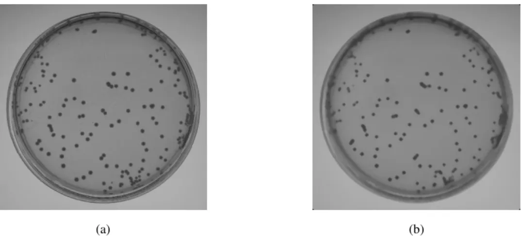
Figure 2: a) Image produced from the beginning for this study (type A) and b) Image obtained from the existing library (type B) [14]. ... 7

Figure 3: Example of an image taken with a dark background and without illumination from below. ... 10

Figure 4: Image capture system created by Chiang et al [14]. ... 11

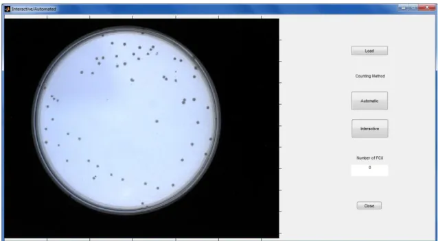
Figure 5: Graphical user interface created for the colony counting. ... 12

Figure 6: a) grayscale result of original image; b) result of the application of median filter. ... 15

Figure 7: result of binarization using Otsu´s method as threshold. ... 15

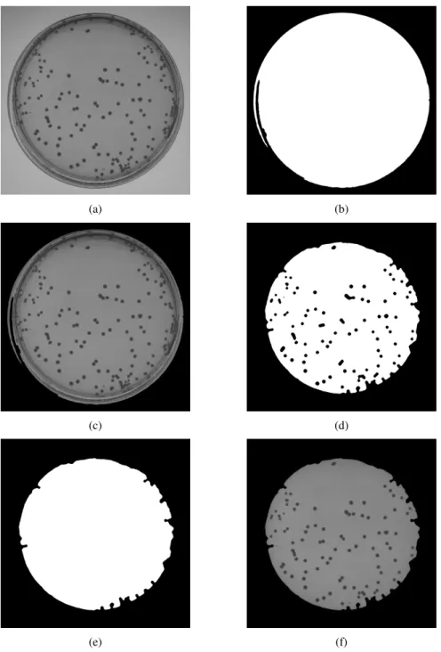
Figure 8:(a) grayscale image of Figure 2(a); (b) mask of Petri dish visualized in (a); (c) image of Petri dish extracted from background obtained as product of (a) and (b); (d) Binarization of (c); (e) mask of central area obtained after hole-filling of (d); (f) image of central area obtained by the product of (c) and (e). ... 16

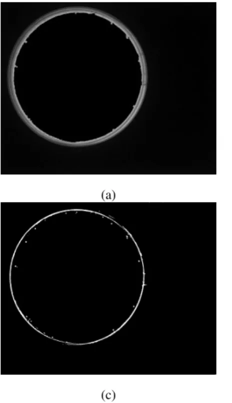
Figure 9: image of rim area obtained by subtracting Figure 8 (c) from Figure 8 (f). ... 17

Figure 10: (a) result of adjusted image intensity values from Figure 8 (f); (b) tresholding results of (a). ... 18

Figure 11: (a) binarization result of Figure 9; (b) rim elimination results of (a). ... 18

Figure 12(a) grayscale image of Figure 2(b); (b) mask of Petri dish visualized in (a); (c) image of Petri dish extracted from background obtained as product of (a) and (b); (d) Binarization of (c); (e) mask of central area obtained after hole-filling of (d); (f) image of central area obtained by the product of (c) and (e). ... 20

Figure 13: (a) result of the application of a close operation on Figure 12(f); (b) result of a difference between Figure 11(f) and (a); (c) thresholding results of (b); (d) final result of elimination of the small non-colony objects of (c). ... 21

Figure 14: (a) image of rim area obtained by subtracting Figure 12 (c) by Figure 12 (f); (b) results of bottom-hat transform of (a); (c) binarization of (b); (d) final image of rim elimination using properties of objects (eccentricity, major and minor axis length and area). ... 21

Figure 15(a) original of type A; (b) result of sum of Figure 10 (b) with Figure 11 (b); (c) original of type B; (d) result of sum of Figure 13(d) with Figure 14(d); ... 22

Figure 16: (a) isolated colonies; (b) clustering colonies. ... 23

Figure 17: clustered colony. ... 24

Figure 18: (a) enlarged example of watershed operation; (b) final result after eliminating the small non-colony pixels. ... 25

(14)

xiv

Figure 20: final result of automatic count. ... 26

Figure 21: (a) beginning of interactive method, where the colonies in green are counted; (b) result of interactive count, where the yellow points are the user´s input. ... 28

Figure 22: (a) final result of interactive method of a simple situation; (b) final result of interactive method of a complex situation. ... 29

Figure 23: result of automatic count. ... 34

Figure 24: result of automatic count. ... 34

Figure 25: result of automatic count ... 34

Figure 26: result of interactive count. ... 35

Figure 29: a) result of proposed automatic system; b) result of OpenCFU system; yellow boxes represent colonies not counted. ... 38

Figure 30: a) original image; b) result of binarization. ... 39

Figure 31: a) result of proposed automatic system; b) result of OpenCFU system; yellow boxes represents colonies not counted. ... 39

Figure 32: a) and b) are results of interactive system; blue boxes represents the colonies counted that previously on yellow boxes were not counted. ... 40

Figure 33 :counting times of manual method and interactive method relatively to the 21 images obtained by Chiang et al. [14]. ... 43

(15)

xv

List of tables

Table 1: Table of confusion summarizing colonies counted manually and automatically. ... 32

Table 2: statistical results of 26 images. ... 37

Table 3: statistical results od 26 images, comparing the results of central and rim area. ... 41

Table 4: percentage of time reduction for the 21 images obtained by Chiang et al. [14]. ... 43

(16)

(17)

1

Chapter 1 Introduction

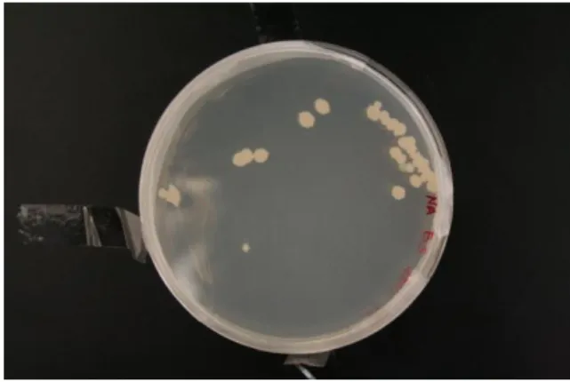
The growth and maintenance of bacteria on agar plates (Petri dishes) has long been a common practice in microbiology. The Colony Forming Unit (CFU) assay is universally recognized as the gold standard method for measuring the effect of radiation on cell viability, environmental control, food and beverage safety assessment and clinical laboratory exams. A significant example is the monitoring or quality control of drinking water, where bacteria such as Escherichia coli, Enterococcus, Cryptosporidium and fecal coliforms are the main indicator of microbiological water quality for human consumption [1]. The culturing process starts by inoculating the specimen to be examined on the agar, thus a solution of the specimen is spread over the agar surface. After inoculation, bacterial cultures are incubated to reproduce good conditions for pathogens bacteria growth. Figure 1 shows a Petri dish with several

Escherichia coli colonies.

(18)

2

considerable fluctuations in results [2]. Due to this, for cultures with high density of colonies, manual counting mostly uses estimation methods, making an extrapolation from a small section of the Petri dish. Automating the detection, counting and analysis of CFU offers significant benefits to eliminate the risk of subjectivity, bias and human.

Figure 1: Petri dish with Escherichia coli bacterial colonies.

(19)

3

1.1. Motivation

Most automatic counting systems perform adequately when the colonies are well spaced, large, circular in shape and with good contrast from the background. When these assumptions are violated, most automatic colony analysis systems can rapidly lose reliability, accuracy and utility. These obstacles include the need to handle confluent growth or growth of colonies that touch or overlap other colonies; the identification of each colony as a unit in spite of differing shapes, sizes, textures, colors and light intensities; the exclusion of colonies around the periphery of the plate reducing statistical accuracy.

To address the above problems, the goal of this study is to design and implement a cost-effective, software-centred system that accepts general digital camera images as its input, for detecting as well as enumerating bacterial colonies in a fully automatic manner. An interactive semi-automatic system is also proposed to overcome any error from the fully automatic system. The proposed systems are capable to reduce the manpower and time required for counting colonies while producing correct colony counting.

1.2. Background

In different fields of microbiology, immunology and cellular biology, counting colonies of cells growing on agar plates is routine. However, everyone who has already counted colonies knows that this is hard work which takes a lot of time. Many groups have thought about an improvement of the counting system and the cited publications certainly won't cover all attempts, but no method has achieved a widespread use at all.

(20)

4

should not be forgotten that the automatic counter methodology will be only an asset, if provides an excellent correlation with the results that would be obtained by a specialist.

The development of automatic counting methods should take into account potential sources of conflict: confluent growth, colonies that touch or overlap the surrounding, and be able to identify and count as being of a different group each colony according the shape, size, texture, color or light intensity. In addition, such methods must be capable of rejecting common artefacts such as imperfections in the agar, dust and edges of Petri dishes. This tool must be designed to deliver a high degree of accuracy in the count, and it is required reliability and reproducibility.

(21)

(22)

(23)

7

Chapter 2 Experimental procedure

In this chapter, it will be explained how the Petri dishes are prepared, and the importance of this preparation, as well as the way of acquiring them. These are very important steps, because if the images do not have quality, the final result could fail in detecting the number of colonies.

2.1. Bacteria culture

For this study, were considered two types of image: type A, which was produced purposely for this work shown in Figure 2(a) and type B obtained from the existing library shown in Figure 2 (b).

(a) (b)

(24)

8

2.1.1. Procedure for images of type A

For the first type of image (type A), Escherichia coli were selected for the experiments. The technique used for the bacterial culture was the spread plate technique. The spread plate method is a technique to plate a liquid sample containing bacteria so that the bacteria are easy to count and isolate. A successful spread plate will have a countable number of isolated bacterial colonies evenly distributed on the plate.

The first step to perform the spread technique was the production of a growth medium. The cultivation and microorganism growth in a laboratory are made in a nutrient material designated by medium culture or growth medium, which should cover the nutritional needs of the growing microorganism which is intended. Generally nutrient sources are necessary, as carbon, nitrogen, minerals and growth factors. These mediums can be prepared or purchased commercially ready for use. Regarding physical state, the growth medium can be solid, semisolid or liquid and can be implemented in petri dishes or test tubes. In this spread technique, the physical condition used was the solid, which are usually obtained by adding a solidifying agent (agar) to a liquid medium. The agar has unique properties; it liquefies at about 100 ° C and maintaining this state until a temperature of 40 ° C. The firm surface of these mediums can enable growth of colonies of individualized way. Therefore, to prepare the growth medium ten Petri dishes were used; each one containing 20 mL of the solution. To produce the solution, 250 mL of growth medium was used (only 200 mL of medium would be needed, but it was used as precautionary measure in case of a mishap). The medium contained 7g of Nutrient Agar in 250 mL of distilled water. It was necessary to adjust the pH of the solution and then to autoclave it for 15min, at 121ºC. To complete the procedure, 20 mL of the medium was distributed in each petri dish.

(25)

9 his paper affirm that to ensure statistical accuracy, the number of colonies must be between 40 and 200. This number allows to get a number of colonies not too large to count completely and the size of colonies must be large enough to facilitate isolation. Then, using a micropipette 10 µL of an each dilution was inserted in its respective Petri dish containing nutritive agar (previously prepared). This small amount was spread, with a spreader, until the culture become uniform. The spreading must be done uniformly, in order to colonies in all area of the Petri dish. To finish, the culture was placed in an incubator for 24 h at 37ºC.

When it is desired to cultivate a culture of a single microorganism (like in this case) it is important that do not exist contamination from the mediums and materials used in the manipulation of the culture and the environment, that is, that work be executed in sterile conditions. All aseptic precautions must comply with two fundamental principles: not to allow micro-organisms in the lab contaminate samples and not allow the cultures being studied contaminate the lab. Consequently, this technique was performed in a laminar flow hood (machine that provides an aseptic work area while allowing the containment of infectious splashes or aerosols) and all the objects that contacted the cultures were previously sterilized.

2.1.2. Procedure for images of type B

(26)

10

2.2. Image acquisition

The objective of this subchapter was demonstrate that it is possible count colonies in an image without having complex acquisition software and allows the user, in any situation, to get an image of a Petri dish and get the count of colonies present therein.

Regarding the image acquisition, for the Type A images, it was done by a normal cell phone. The Petri dish was placed over a white light, with the purpose of illuminating this. Then the photo was taken with a 5 megapixel cell phone. The result is shown in Figure 2 (a). Before that, was experimented a dark background without illumination from below (Figure 3).

Figure 3: Example of an image taken with a dark background and without illumination from below.

It is possible observe in Figure 3, that the image presents some reflexes. That would be a problem during the phase of image processing, making the segmentation of the colonies a difficult process.

(27)

11 Figure 4: Image capture system created by Chiang et al [14].

Chiang et al. [14] did an image capture system to obtain the culture photos (Figure 4). In order to accentuate the region of interest and provide adequate contrast between the colonies and the background, the plate was illuminated from below by a LED panel light, due to is uniform illumination and thin shape. Platform 1 was then used to fix the position of the plate. Since the plate is covered with a lid with a diameter slightly bigger than that of the plate, to take the image inside the plate, platform 2 with the same diameter as the bottom plate was placed just above the lid to exclude the image of the lid.

The main purpose of the design of this apparatus is to obtain the images inside the periphery of the plate, including the edge of periphery. Finally, external light was blocked with the cover, and a CCD camera with 1.3 million effective pixels (1280 (H) × 1024 (V)) was used to capture the images [14].

2.3. Graphical user interface

(28)

12

created by default, two files, .m e .fig. The first contains the code developed interface. The second can be used to change the visual aspect of the application through the GUIDE. For each object a callback function is created. Here it should be put the code that want to run when the object is called.

A main objective of this work was to create software that is easy to use for anyone, be it the expertise about image processing or not. The literature has already colony counting software, such as NICE and OpenCFU, which are adaptive applications, it means, there are certain parameters such as the threshold, which can be adjusted depending on the image displayed. This can be seen as an advantage of the software but if the user does not have a background in image processing may become difficult to use the software. For this study, it was then created non-adaptive software where the user only needs to load the image using the "Load" button, and choose the counting method. If the user presses the "Automatic" button get a completely automatic counting and if the user presses the "Interactive" button then this gets a semi-automatic count, and it will be need the user´s input on the image to count the colonies not counted. The result of the count is shown in a text box and to close the application there is a button "close". This makes it easy to use for anyone and can be used by people with no background in image processing.

(29)

13

Chapter 3 Colony counting methods

3.1. Automatic method

The next subchapter represents the methods used to count colonies automatically. After opening the image on the application (Figure 5), the user can opt if they want an automatic count or an interactive count. Choosing the automatic method provides the user to obtain the colonies counted very quickly. Next, it is presented the cluster colony partition, where the isolated colonies are separated from the clustered colonies and the colony counting where it is explained how the automatic method counts.

Before performing the pre-processing, it was necessary to distinguish the two types of images because they had different characteristics. Type A images had a light background shown in Figure 2 (a) and type B had a dark background shown in Figure 2(b). Therefore, the first step of the whole method was to estimate the mean of the 3 components of the image (components RGB). It was noted that the mean of the 3 components for the type A images was bigger than 120 (the grayscale of the images range from 0 to 255). So, this was the parameter chosen to distinguish the two types of images. After the distinction, each type of image had its own pre-processing and segmentation.

(30)

14

complex than those used for the center. Then, the pre-processing of the image is divided into two parts: the area in the center of the image and the rim area.

3.1.1. Preprocessing and segmentation for type A images

In this study, the RGB image (color images) (Figure 2 (a)) was converted into a grayscale image (Figure 8 (a)). The goal of this method (pre-processing and segmentation) was to divide the images of the Petri dishes into two parts, the central area and the rim area, from the image, and to segment the colonies (in the image where the colonies appear in white and the background in black) and it was based on reasoning used by Chiang et al [14]. Geissmann Q [13] and Clarke et al. [11] in its methods (Open CFU and NICE, respectively) did not separated the image in two parts, they divided the image in sub-regions.

First, masks from the original images were created with the purpose of multiplying them with the grayscale image to remove the background. To get the mask, a median filter was applied, with the goal to remove pixel noise, Clarke et al. [11] used a Gaussian smoothing function and Geissmann Q [13] used a median filter. In the Figure 6, it is possible to the result of the application of the median filter on a) obtained b). Median filtering is a nonlinear operation often used in image processing, because simultaneously reduce noise and preserve edges. The main idea of the median filter is to run through the image pixel by pixel, replacing each pixel with the median of neighboring pixels. The next phase was threshold binarization. To perform this, it used

(31)

15

(a) (b)

Figure 6: a) grayscale result of original image; b) result of the application of median filter.

The second step of the method was to separate the central area of the Petri dish from the rim area. The grayscale image in Figure 8 (c) shows that the background of the rim area is darker than that surrounding the central area, therefore, threshold binarization can be used to separate the central area from the rim area. The value of threshold used was a fixed value (0.45). This value was chosen because worked well on the all 5 images. In the Figure 8 (c), it is possible to see the image before the binarization, and in the Figure 8 (d) the result of 0.45 as threshold. The Figure 7 shows the result of the binarization if it was used Otsu´s method. Figure 8 (f) shows only the central area and it is the result of the multiplication between Figure 8 (c) and Figure 8 (e) (this image, visualized in Figure 8 (e) is the result of the filled holes of Figure 8 (d)).

With the location of pixels in the central area, the rim area can be obtained by subtracting the central area (Figure 8(f)) from the Petri dish area (Figure 8(c)). The resulting image is shown in Figure 9.

(32)

16

(a) (b)

(c) (d)

(e) (f)

Figure 8:(a) grayscale image of Figure 2(a); (b) mask of Petri dish visualized in (a); (c) image of Petri dish extracted from background obtained as product of (a) and (b); (d) Binarization of (c); (e) mask of central area obtained after

hole-filling of (d); (f) image of central area obtained by the product of (c) and (e).

(33)

17 Clarke et al. [11] system is an adaptive system, which the user can choose the thresholding method, between Gaussian distribution (standard derivation from 3 to 6), Otsu and manual.

Figure 9: image of rim area obtained by subtracting Figure 8 (c) from Figure 8 (f).

(34)

18

(a) (b)

Figure 10: (a) result of adjusted image intensity values from Figure 8 (f); (b) tresholding results of (a).

The main problem of the extraction was the colonies overlapping with the extremities of Petri dish, because in these images, they have the same gray value.

In the NICE method, Clarke et al. [11] combined extended minima and thresholding algorithms to segment the colonies. The extended minima function was used to find the center of colonies which could be considered regional dark points. This regional method allowed identifies colonies based on the local contrast.

(a) _(b)

(35)

19

3.1.2. Pre-processing and segmentation for type B images

The method used in this pre-processing was similar to the previous method, based on the study made by Chiang et al [14].

Firstly, it was necessary to create a mask of the Petri dish, with the purpose of removing it from the background. This mask was created by threshold binarization of Figure 12(a). The value of threshold used was 0.98 and it was a fixed value, because this value worked well in all 21 images. To extract the Petri dish from the background, this mask was multiplied by the image in grayscale (Figure 12(a)), with the result shown in Figure 12(c). As in the previous images, the rim area is darker than the central area, so, to separate the two areas another binarization, with a fixed threshold with the value of 0.7, was applied, in Figure 12(c). The result is shown in Figure 12(d). After filling the holes, the mask of the central area (Figure 12(e)) was obtained. To get the final image of the central area (Figure 12(f)), the mask shown in Figure 12(e) was multiplied by Figure 12(c).

(36)

20

Figure 12(a) grayscale image of Figure 2(b); (b) mask of Petri dish visualized in (a); (c) image of Petri dish extracted from background obtained as product of (a) and (b); (d) Binarization of (c); (e) mask of central area obtained after

hole-filling of (d); (f) image of central area obtained by the product of (c) and (e).

The rim area (Figure 14(a)) was obtained as with the previous method, by subtracting Figure 12(c) by Figure 12(f). To extract the colonies from the rim area, the bottom-hat transform was applied. This method is similar to the one used previously in the extraction of the colonies from the central area. The next step was the binarization in Figure 14(b) with the results shown in Figure 14(c). The threshold used in this binarization was estimated by the Otsu´s method. This algorithm assumes that the image contains two classes of pixels following bi-modal histogram (foreground pixels and background pixels), then calculates the optimum threshold separating the two classes. To obtain only the colonies, the same line of thought that was used to extract the colonies from the rim in the previous image was used, where the eccentricity, the

(a) (b)

(c) (d)

(37)

21 major and minor axis length and the area of each object were used. The results are shown in Figure 14(d)

(a) (b)

(c) (d)

Figure 13: (a) result of the application of a close operation on Figure 12(f); (b) result of a difference between Figure 11(f) and (a); (c) thresholding results of (b); (d) final result of elimination of the small non-colony objects of (c).

(a) (b)

(c) (d)

Figure 14: (a) image of rim area obtained by subtracting Figure 12 (c) by Figure 12 (f); (b) results of bottom-hat transform of (a); (c) binarization of (b); (d) final image of rim elimination using properties of objects (eccentricity,

(38)

22

The images from Figure 15 are the results of segmentation and the corresponding original image. Figures 15 (b) and (d) are the results of the sum of colonies extracted from the central area with the colonies extracted from the rim area. These two images were used in the separation phase, explained in the next chapter.

(a) (b)

(c) (d)

Figure 15(a) original of type A; (b) result of sum of Figure 10 (b) with Figure 11 (b); (c) original of type B; (d) result of sum of Figure 13(d) with Figure 14(d);

3.1.3. Clustered colony partition

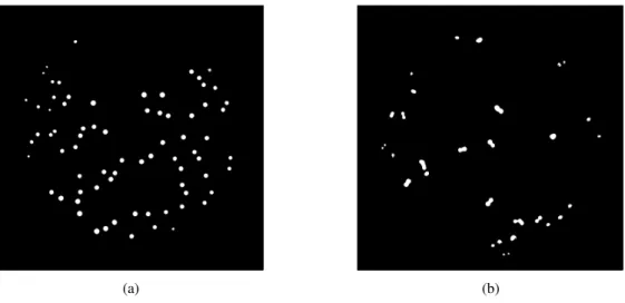
In this phase the objective was to create two different images, one of them contains the isolated colonies (Figure 16(a)) and the other containing the overlapping/clustering colonies (Figure 16 (b)).

(39)

23 actually a circle, while an ellipse whose eccentricity is 1 is considered a line segment. The mean of eccentricity of a normal colony has a value close to 0.25, and normally a clustered colony has a value higher than 0.5. In Figure 17, it is possible to see a clustered colony with a value of eccentricity of 0.8. Normally, the area of a clustered colony is higher than the mean areas of all colonies. Therefore, with these two characteristics, if an object in an image was an eccentricity higher than 0.5 or an area of an object was higher than the mean of the areas plus half of the mean areas, this object was considered a clustered colony, if not the object was an isolated colony.

(a) (b)

Figure 16: (a) isolated colonies; (b) clustering colonies.

(40)

24

Figure 17: clustered colony.

3.1.4. Colony counting

Brugger et al. [12] to count colonies used a Bayes classifier, which is a probabilistic classifier based on Bayes theorem. It was used some properties such as ratio between major and minor axis to determine how many colonies are in the group. In the other hand, Chiang et al. [14] used watershed transform to separate the clustered colonies and proceeding then to the count. In his study, he obtained greats results with this method.

To count the single colonies present in Figure 16 (a), as the colonies are all individual, was used a function that finds connected components in binary image and estimate the number of objects that exist on an image. The result of application of this function shows a structure with 4 elements. The first one is the connectivity of the connected objects, the second one is the size of the image, the third one is the number of objects presents in the image and the last one is a cell array the kth element in the cell array is a vector containing the linear indices of the pixels in the kth object. To obtain the number of objects on an image, it is necessary get the third element referent to the number of objects in an image.

(41)

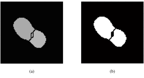
25 input image, except that the gray level intensities of points inside foreground regions distance are changed to show the distance between that pixel and the nearest nonzero pixel. Monteiro [16], in his PhD thesis explains the watershed transform, and inside this watershed, explains two strands: the immersion watershed and the rainfall watershed. In this study, the watershed used was the immersion watershed and it is when sinking the whole surface slowly into a lake water leaks through the holes, rising uniformly and globally across the image, and proceeds to fill each catchment basin. Then, in order to avoid water coming from different holes merge, virtual dams are built at places where the water coming from two different minima would merge. When the image surface is completely flooded the virtual dams or watershed lines separate the catchment basins from one another and correspond to the boundaries of the regions. The watershed operation computes a label matrix identifying the watershed regions of the input matrix, which can have any dimension. The elements obtained are integer values greater than or equal to 0. The elements labeled 0 do not belong to a unique watershed region. These are called watershed pixels. The elements labeled 1 belong to the first watershed region, the elements labeled 2 belong to the second watershed region, and so on. In Figure 18(a) it is possible to see a result of watershed operation on a clustered colony. The operation divided the object in 3 parts, even though visually the object seemed to have two colonies together. The small object formed after the application of the watershed, was eliminated through the mean area of the isolated colonies (Figure 16(a)). The result is shown in Figure 18(b).

(a) (b)

(42)

26

Although the watershed operation worked well for objects with few colonies (2, 3 or 4), when the cluster had a lot of colonies, the watershed did not divide uniformly (Figure 19(b)). To bypass this problem, the mean area of isolated colonies in Figure 16 (a) was calculated. This mean area is the mean area of an isolated colonyin the related image so the big areas, like Figure 19 (b) were divided by the mean area obtained in the image with the isolated colonies. These estimated results were summed to the count of the watershed operation, and then summed to the count of isolated colonies. The final result is shown in Figure 20, where all counted colonies appear in green.

(a) (b)

Figure 19: (a) example of a clustered colony with a big area (inside the black box); (b) result of watershed operation for the clustered colony inside the black box.

(43)

27

3.2. Interactive method

The next sub-chapter explains the methodology for conducting interactive method. This method combines automatic parts with interactives parts between the user and the system / computer. For this method to be used, the user must press the button of the interactive method presented in the application.

The preprocessing step was the same used on the automatic method, in section 3.1.1 and 3.1.2. To separate the isolated colonies of clustered colonies, was used the methodology explained in section 3.1.3, clustered colony partition, where the eccentricity and the average of the areas of each object was used. If an object had a higher eccentricity than 0.5 or an area of an object was higher than the mean of the areas plus half of the mean areas, then the object was considered as clustered colonies (Figure 16(b)), if not it is considered a single colony (Figure 16(a)).

The followed section represents the methods used to count the colonies interactively.

3.2.1. Colony counting

The result of colony clustered partition shows two images, one of them containing single colonies and other grouped colonies. To count the image of individual colonies, the procedure is the same method used in section 3.4, Colony counting, where was used to function that finds connected components in binary image and estimate the number of objects that exist on an image.

(44)

28

or delete keys for the keyboard. The point is eliminated from the picture as the count. To finish the interactive count, the user must press the enter key from the keyboard.

(a) (b)

Figure 21: (a) beginning of interactive method, where the colonies in green are counted; (b) result of interactive count, where the yellow points are the user´s input.

Figure 22 shows two interactive count results, being (a) considered the result of a simple count and (b) considered the result of a complex count.

In Figure 22 (a) it is observed that most of the colonies are already counted by the automatic part of the interactive method. It is observed that there are few clustered colonies in the image being constituted mainly of single colonies. It is also possible to verify that there are a reduced number of colonies at the edge of the Petri dish. In this case, the use of interactive method becomes a simple case because in 65 colonies, the user only needs to count, by click, about 15. This causes a reduction in 50% of count time, compared to manual counting.

(45)

29

(a) (b)

(46)

(47)

31

Chapter 4 Results and discussion

The practical application of an image segmentation algorithm requires that we understand how its performance varies in different operating conditions. Evaluating algorithms allows researchers to know the strengths and weaknesses of a particular approach and identifies aspects of a problem where further research is needed [16].

In this evaluation, 26 images of colonies in Petri dishes were used. These images were counted automatically by the proposed systems and also manually by Biomedical Engineering students. To evaluate the performance of the two proposed methods, the results obtained were compared with two other automatically counting systems (NICE and Open CFU).

4.1. Methods used in statistical analysis

(48)

32

Chiang et al. [14] in his study used the statistical results of precision, recall, f-measure and APE to evaluate his results. To compute precision and recall, it is necessary to determine which true positive pixels are correctly detected, and which detections are false or missing. The precision is related with the false positive values, and in this case they are colonies that the system identifies but that do not exists. The recall is related with the false negatives and represents the colonies that were not identified. In probabilistic terms, precision is the probability that the result is valid, and the recall is the probability that the ground truth data was detected. A low recall value is typically the result of under-segmentation and indicates failure to capture salient image structure. Precision is low when there is significant over-segmentation, or when a large number of boundary pixels have greater localization errors than some threshold [16].

Table 1: Table of confusion summarizing colonies counted manually and automatically.

Table of confusion Manual counting

True False

Automatic couting Positive True Positive (correct result) False positive(unexpected result) Negative False negative(missing result) True negative(correct absence)

The equations used to obtain the precision (measure of exactness) and recall (measure of completeness) [14], are defined as:

(1)

Precision = _{Total number of components retrieved}Number of colonies retrieved

= _{True positive + False positive}True positive

(2)

Recall =_{Total number of existing colonies =}Number of colonies retrieved _{True positive + False negative}True positive

(49)

33 (3)

F − measure =_{α ∗ precision + (1 − α) ∗ recall}precision. recall

where α determines the relative importance of each term. Following Martin et al [17], α is selected as 0.5 expressing no preference for either.

The absolute percentage of error (APE) is the most appropriate information about average percentage errors which are used to a great extent in reporting accounting results. Makridakis S. [18] defined a new equation to obtain the absolute percentage of error, and it is defined as:

(4)

𝐴PE𝑡 = |_(𝐴𝐴𝑡− 𝐹𝑡

𝑡+ 𝐹𝑡)/2| ∗ 100

where _𝐴_𝑡 is the actual value and it is represented as the manual counting obtained and _𝐹_𝑡 is the forecast value, which is the counting obtain by the automatic methods.

4.2. Results of Automatic method

The functioning of automatic method depends largely on the type of image. Features such as the number of colonies at the edges of the Petri dish, the number of clustered colonies, and the contrast in the image interfere with the performance of the method.

In Figure 23, is shown result of the automatic counting for a relatively simple image. It is possible to observe that the colonies present spread throughout the area and widely spaced. Furthermore, there are few colonies on the edge, which facilitates the automatic counting. Another feature of this picture is that there are very few clustered colonies. In this case, the value of APE is about 0.6%, a very low, almost close to perfect.

(50)

34

Figure 23: result of automatic count.

Figure 24 shows an image with an average degree of complexity. In this image the automatic method has an APE of 17%. This happens due to little contrast existing in the image. It presents a considerable number of clustered colonies, making it difficult to hit in the count. In this case, the number of colonies in the edge of Petri dish is low.

Figure 24: result of automatic count.

(51)

35 Figure 25 shows the result of automatic counting for an image with a high degree of complexity. It is possible to observe that about 50% of the colonies are not counted by this method and APE in this case around 50%. In this image, there are many clustered colonies also are at the edge. The difficulty of the automatic method is counting colonies on the edge.

.

4.3. Results of Interactive method

One goal of this work was to create a method to reduce the counting time but had a percentage great success.

The interactive method, the APE is always very close to zero. So the complexity of the counts is measured as the time that each delay.

Figure 26 shows an image in where the interactive method don´t present a big reduction of time. Although, it is possible to observe that the automatic part of the interactive method left a small number of colonies per count, which acilitates the work of the user. This is because there are no colonies on the edges and besides there are only two groups of clustered colonies. The results for the 26 images are presented in Appendix D.

Figure 26: result of interactive count.

(52)

36

interactive method provides some colonies for the user select. These colonies are mainly clustered colonies.

Figure 27: result of interactive count.

When the number of clustered colonies is high, is presented to the user a high number of colonies to count. This causes the small reduction of the counting time. In the Figure 28, there is shown the result of an interactive count, where a large number of clustered colonies. In this case, the user had to rely manually 366 colonies. Although a relatively large number, the user achieves a 36% reduction in the count time while maintaining accuracy.

(53)

37

4.4. Evaluation

In this subchapter, it will be compared all the methods used in this study. Measures relatively to the statistical results and also time will be studied.

The Table 2 shows the results of Precision, Recall, F-measure and APE for each method, approached in this study, in relation to the 26 images. In the Appendix B it is shown the individualized results for the 26 images for the 4 methods studied (Table B1 the automatic results, Table B2 interactive results, Table B3 OpenCFU results and Table B4 NICE results). The first step to obtain these statistical values was the manual count. This was performed by different students of Biomedical Engineer. The results were obtained by comparing each manual count with the other 2 counts. To calculate the values for the other 4 methods, the automatic count of each method was obtained for the respective software. Then, this count was compared with the 3 different manual counts. The individualized results for the 26 images are shown in Appendix A. The results shown in table 2 are the mean of the calculated values.

Table 2: statistical results of 26 images.

Measure

Method

Manual Automatic Interactive NICE OpenCFU Precision 0.9879 0.9848 0.9808 0.9607 0.9915

Recall 0.988 0.8698 0.9937 0.878 0.918

F-measure 0.9876 0.9188 0.9869 0.9055 0.9514 APE (%) 2.4937 16.3128 2.3272 18.914 9.7067

Observing the table 2 results, it is possible to affirm that in relation to Precision, the results are similar, although the NICE method has the lowest value. This means that the colonies counted normally are correct, being the number of false positives a low value.

(54)

38

possible to conclude that these 2 methods fail in the identification of some colonies. The OpenCFU method has an acceptable result for the recall with a higher than 0.90. In contrast to these three methods, the Interactive presents a value close to the manual value.

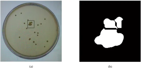
Figure 29 shows the results of the proposed automatic method and the OpenCFU. It is possible to observe in the yellow box that both methods fail in the detecting some colonies in the rim area of Petri dish. These failures, contribute to the high number of false negatives and thus the low Recall value. It is also possible to see that OpenCFU detects a higher number of colonies in the rim area than the proposed automatic system. The explanations for these detection failures are the fact that some of the colonies are eliminated in the pre-processing step due to its color which is similar to that of the edges of the Petri dish. An example it is shown in Figure 30, where it is possible to see the original image and the image after a binarization. The colonies that appear in the yellow box in a) are attached to the edge of the Petri dish (Figure 30 b)).

(a) (b)

(55)

39

(a) (b)

Figure 30: a) original image; b) result of binarization.

Another failure that contributes to the low Recall values of the proposed automatic system and also observed in the OpenCFU method, is the fact that in some cases, the system does not identify some colonies in the central area (observed in the yellow boxes), shown in Figure 31. Analyzing the images, it can be concluded that these problems exist due to the low contrast in the image. The non-identified colonies are practically the same color as the background, which makes it difficult to segment them. To improve this method and avoid these problems, the contrast has to be increased thereby facilitating the identification of these colonies.

(a) (b)

Figure 31: a) result of proposed automatic system; b) result of OpenCFU system; yellow boxes represents colonies not counted.

(56)

40

colonies is estimated by averaging the areas of isolated colonies. This estimate does not always get the best results, counting down the number of colonies. This problem also influences the false negative numbers.

(a) (b)

Figure 32: a) and b) are results of interactive system; blue boxes represents the colonies counted that previously on yellow boxes were not counted.

A huge advantage of the interactive system is the ability to fix these failures, which occur in the proposed automatic system and in the OpenCFU. After the automatic count, the user can correct the missed colonies. Figure 32 shows the result of the interactive count, and comparing it to Figure 29 and 31, it is possible to observe that in the interactive method, the colonies that were missing in the rim and central areas, shown in the yellow box are marked and counted (blue box).

Analyzing the F-measure (table2), the relation between Precision and Recall, as expected, the Interactive method presents the best value, close to the manual count, due to its great values of Precision and Recall. The OpenCFU method has an acceptable result through its good Precision result. The NICE presents the worst result due to its low recall value and the automatic proposed system, despite the low recall value has an F-measure higher than the NICE.

(57)

41 Table 3: statistical results od 26 images, comparing the results of central and rim area.

Measure

Method

Manual Automatic

All area Central area Rim area Precision 0.9879 0.9848 0.9659 0.9615

Recall 0.988 0.8698 0.9064 0.636

F-measure 0.9876 0.9188 0.9288 0.7248 APE (%) 2.4937 16.3128 14.233 55.0449

One of the first steps of the proposed automatic method was the separation of the original image in two images, one of them containing the central area of the Petri dish and the other one containing the rim area. As the proposed automatic method has different results to the manual count (Table 2) an individualized study of these two different areas was necessary, to determine whether the method fails in the central, rim or in the whole area. In Table 3, the first column refers to the manual count, column 2 shows the results of the automatic count analyzing the image as a whole, and column 3 shows the results of the central area and the last column the rim area.

In relation to the Precision values, it is possible to observe that both in the central area as well as in the rim area the results are lower comparing with the results of the automatic count of the whole area. As the values of the central and rim areas are similar, it is not possible to confirm where the automatic system works better.

Analyzing the Recall value, of the automatic system, the central area has a value greater than the rim area. In this case, the rim area has a really low value, around 0.636. Observing the result of the recall to the whole area, around 0.8698, it is possible to conclude that this low value is influenced by the result of the value of the rim area. The false negatives on the rim area have a high value, comparing to those of the central area. Being the F-measure the relation between Precision and Recall, the results observed in Table 3 are the expected.

(58)

42

To improve the results of the automatic count, the method applied to the rim area needs to be modified in order to reduce the number of false negatives. Even the system applied to the central area needs to be modified to improve the results. It is possible to conclude that the system fails mainly in the rim area but the central area can be improved too.

As previously explained, the manual count is a time-consuming process, which can at times take up many human hours; for example, the time needed to count all 26 images is around 71 minutes. The manual counting time depends on the experience of the researchers, the number of colonies present in a Petri dish and the number of aggregated colonies. The counting time of the interactive method of this study depends on the number of aggregated colonies, the number of colonies that part of this method can automatically count and the speed and system performance. One of the main goals of this study was the time reduction, to protect the human against tedious work.

Figures 33 and 34 show the box plots of the time that the manual method and the Interactive method took to count each image. A box plot is a way of graphically depicting groups of numerical data through their quartiles. Box plots may also have lines extending vertically from the boxes indicating variability outside the upper and lower quartiles. Observing the graphics in Figures 33 and 34, the blue box represents 50% of all analyzed values. The base of the box is the lower quartile and represents 25% of the values, the top of the box is the upper quartile and represents the 75% of the observed values and the line presented in the middle of the box is the average and divides the bottom half from the upper half of the sample. The straight vertical line connects the top of the box to the highest value observed and the other line connects the bottom of the box at the lowest observed value, this segment is called Whisker. Box diagram is a tool for outlier detection, which are represented by the black points.

Figure 33 represents the time that each method took to count the 21 images obtained by Chiang et al. [14] and Figure 34 represents the time that the methods took to count the 5 images created for this study. The time of study of the two different libraries was divided because these had different pre-processing methods which caused a significant difference in time. The reduction of time that each method allows in each image is shown in the Appendix C.

(59)

43 50 and 150 seconds. The median observed in the two boxes is different too, while the median of the manual method is 129 seconds, the median of interactive method is 81 seconds. It is also observed that two outliers exist above the box. These values are from the count of the images with more colonies. In the interactive method, this time is reduced too.

Figure 33 :counting times of manual method and interactive method relatively to the 21 images obtained by Chiang et al. [14].

Table 4 shows the total time reduction for the 21 images of each of the proposed methods, automatic and interactive, in relation to manual counting. The average of the automatic count is about 6 seconds, hence a 94.14% reduction in count time. This is a huge time reduction, enabling the researcher a quick count. Regarding the interactive method, this presents a significant reduction in time, around 40%, which allows for relieving the user’s workload.

Table 4: percentage of time reduction for the 21 images obtained by Chiang et al. [14]. Method Time reduction (%)

Interactive 40.10 Automatic 94.14

(60)

44

seconds to be counted. This time is the maximum for the manual method. For this same image, watching the interactive method, the time is reduced to 110 seconds (maximum of the box).

Figure 34: counting times of manual method and interactive method relatively to the 5 images obtained for this study.

Looking at table 5 it can be concluded that in the case of the automatic method the time reduction for the count of the 5 images is 83.73% and 33.46% in the case of the interactive method. These results are worse than the results for the 21 pictures, due to the fact that these images present an inferior quality to those obtained by Chiang et al. [14]. These have a higher amount of noise, a higher number of colonies on the edge of the Petri dish and a larger quantity of aggregated colonies, requiring different and harder pre-processing work, making the system slower.

Table 5: percentage of time reduction for the 5 images obtained for this study. Method Time reduction (%)

Interactive 33.46

Automatic 83.73

(61)

45 method a reduction of around 40%. In the images obtained for the purpose this study, the reduction is less (about 83% for the proposed automatic method and about 33% for the interactive method). This is due to the fact that the pre-processing is different. As the obtained images had a higher noise level a stronger pre-processing was done, which slowed down the system.

Analyzing all the methods, it is possible to observe that the main advantages of the interactive method are the precision values, the recall, the F-measure and the APE. These values are really close to the manual counts. This method has the advantage of counting colonies that the other methods do not count; fixing failures such as correctly identifying how many colonies exist in the aggregate count, the overlapping colonies on the edge of the Petri dish and counting the colonies even when the contrast is not too big.

(62)

46

big time saver, in some cases exceeding 50% while maintaining the robustness and reliability of the count.

The user’s decision should be considered in the choice of the software. Features like the way the results are presented, the complexity of use and esthetics are important in the choice of the software. In this case, as the users of these applications are typically researchers in chemistry and microbiology, the software must be easy to understand, because normally they do not have much background in image processing. In this perspective, the proposed method is easy to use where only the choice of the counting method is required. If the chosen method is the automatic one the software then returns the value and the colonies appear marked in green while if the chosen method is the interactive one, the count has to be completed by counting the unmarked colonies. The OpenCFU software is also easy to use, automatically counting the colonies and presenting them in a little blue box, having the advantage that if the user has image processing concepts, to be an adaptive software where you can choose between three thresholds (normal, inverted and bilateral), as well as drawing areas of interest. If the user does not have image processing background the software becomes more complex. Analyzing NICE, it is a difficult to use software, where the selection of the threshold value (manual or by one of the software methods) requires the user to have image processing knowhow. Additionally, colonies appear unmarked, thereby making it difficult to identify software failures.

(63)

47

Chapter 5 Conclusion and future research

This dissertation focuses on simplifying bacterial count problems using two methods, a fully automatic one and the other interactive. Another two methods (NICE and OpenCFU) were studied in order to compare them to the created methods.

Normally, this tedious, time-consuming and error-prone method count is performed manually by researchers. Automatic methods have been studied and created to facilitate the task of researchers. A user-friendly GUI was also developed for the proposed method.

The proposed automatic method presented some good results in the quantification of

E. coli colonies. It presents a high precision value of around 0.98, the number of false

(64)

48

The NICE system presents the worst results, mainly because of the high number of false negatives, which makes the recall a bad value, around 0.878. With this study, it can be concluded that NICE system is not recommended for researchers who do not have image processing knowledge, because apart from the low results, it is a difficult to use system, where the user needs to choose the threshold and the counted colonies do not appear marked, making it difficult for the user to identify the uncounted colonies.

The OpenCFU is the fully automatic method that produces the best results, with a high precision value, an acceptable value of the recall measure and an absolute percentage of error of around 9%. It is a system that reduces the counting time and is user-friendly.

The interactive method was found to be capable of counting the number of E. coli colonies within an acceptable absolute percentage of error, 2.3272%. The mean values of precision, recall, and F-measure are all bigger than 0.98. The Interactive method shows similar results to those of human count because it allows for the correction of the false negatives of the other methods. This method is capable of reducing the counting time by 40% for the 21 images obtained by Chiang et al. [14] and by 33% for the 5 images created for this dissertation. The human interaction with the system is also a simple task, since the user only has to click on the unmarked colonies and these are added to the previously counted ones.

The choice of the method is up to the user; if you need a count where accuracy is more important than the time spent, the best method in this case is the interactive one. If accuracy is not as important as the time spent, then the method that produces better results with a large reduction in time is the OpenCFU.

The results obtained in this study, suggested that there are many problems to be solved in the proposed automatic bacterial count and some improvements to be made in the interactive system.

In the image acquisition, the researcher has to be careful to obtain images with the least possible noise and maximum possible contrast. The acquisition method of Chiang et al. [14] works fairly well, although sometimes the image presents little contrast. In a future study, it would be more interesting to have pictures from day to day cameras, like cell phones, and work with them in a system. Although this study presents images taken with a mobile phone, high noise is present.

(65)

49 separating it into two. Thus, it would be possible to identify colonies more easily, providing it is a small area, even if the contrast is low, identification is possible. Another issue to be considered in the future is if it would be better to have an adaptive counting system or not. The system created for this job is a non-adaptive system. The big advantage is that it is easy to use, even by researchers without expertise in the image processing area. The problem is that it works well for 26 images, but if you add a different image it no longer works. I think the future is to create a non-adaptive system but that works well for almost all types of images and colonies.

The work presented in this dissertation provides a new approach, the Interactive count system, is based on the interactivity between user and system. This method presents some good results, although it can be improved. The interactive method displays an image containing the counted isolated colonies and colonies grouped or that are unidentified or uncounted in the rim area. In some images, the number of colonies per count is relatively high, leading the user to spending little time counting. In future work, it would be interesting to develop a more accurate, automatic method, where only at the end of the automatic count would the interactive part act, correcting the false negatives and discounting false positives. Thus, the time required for the interactive method would be reduced and would it be possible to further improve the results.

(66)

(67)

51

References

[1] EPA, Water quality standards and revision, Washington, DC, 2006.

[2] J. M. Bewes, N. Suchowerska e D. R. McKenzie, “Automated cell colony counting and analysis using the circular Hough image transform algorithm (CHiTA),”

Physics in Medicine and Biology, vol. 53, pp. 5991-6008, 2008.

[3] M. Putman, R. Burton e M. H. Nahm, “Simplified method to automatically count bacterial colony forming unit,” Journal of Immunological Methods, vol. 302, pp. 99-102, 2005.

[4] N. K. Uppal e R. Goyal, “Computational approach to count bacterial colonies.,”

International Journal of Advances in Engineering & Technology, vol. 4(2), pp. 2231-1963, September 2012.

[5] G. Corkidi, R. Diaz-Uribe, J. L. Folch-Mallol e J. Nieto-Sotelo, “COVASIAM: an

Image Analysis Method That Allows Detection of Confluent Microbial Colonies and Colonies of Various Sizes for Automated Counting,” Applied and

Environmental Microbiology, vol. 64(4), pp. 1400-1404, April 1998.

[6] J. Marotz, C. Lubbert e W. Eisenbei, “Effective object recognition for automatic countingof colonies in Petri dishes (automatic colony counting),” Computer

Methods and Programs in Biomedicine, vol. 66, pp. 183-198, 2001.

[7] P. R. Barber, B. Vojnovic, J. Kelly, C. R. Mayes, P. Boulton, M. Woodcock e M.

C. Joiner, “Automatic counting of mammalian cell colonies,” Physics in Medicine

and Biology, vol. 46(1), pp. 63-76, 2001.

[8] J. Dahle, M. Kakar, H. B. Steen e O. Kaalhus, “Automatic counting of mammalian cell colonies by means of a flat bed scanner and image processing,” Cytometry, vol. 60(A), pp. 182-188, 2004.

[9] C. Zhang e W.-B. Chen, “An Effective and Robust Method for Automatic Bacterial Colony Enumeration,” International Conference on Semantic Computing, pp. 581-588, 2007.

InteractiveAutomated Method to Count Bacterial Colonies