School of Social Sciences
Department of Political Economy
Determinants of Household Debt in Portugal
Dissertation submitted as partial requirement for the conferral of Master in
Monetary and Financial Economics
by
Ana Luísa Romão
Supervisor:
PhD Ricardo Barradas, Assistant Professor
ISCAL-IPL
2 RESUMO
A dívida das famílias em Portugal aumentou gradualmente, especialmente após a crise financeira de 2007-2008. Em 2018, cerca de 11 anos após a crise, ainda existem altos valores de endividamento das famílias. Nesse sentido, esta dissertação realiza uma investigação empírica para avaliar os determinantes da dívida das famílias em Portugal, através de uma análise econométrica de séries temporais para o período entre 1989 e 2018. De forma a levar em consideração todas as hipóteses referidas na literatura que explicam o endividamento das famílias, foi construída e estimada uma equação para testar sete hipóteses (preços das casas, ativos financeiros, salários em queda, estrutura etária, redução do bem-estar, taxa de juro baixa e expenditure cascade). Os resultados obtidos indicam que o salário é o determinante mais robusto a longo e a curto prazo. A longo prazo, uma diminuição dos salários causa um aumento da dívida das famílias portuguesas. A curto prazo, um aumento nos salários causa um aumento na dívida das famílias portuguesas. Também a curto prazo, verifica-se que os preços das casas têm um forte impacto na dívida das famílias portuguesas. Relativamente a longo prazo, também se verifica que a taxa de juro e a redução do bem-estar social têm um impacto significativo na dívida das famílias.
Palavras-chave: Dívida das famílias, preços das casas, ativos financeiros, salários em queda, estrutura etária, redução do bem-estar, taxa de juro baixa e expenditure cascade, Portugal, modelo ARDL.
3 ABSTRACT
Household debt in Portugal has increased gradually, especially after the financial crisis of 2007-2008. In 2018, about 11 years after the crisis, there are still high values of household indebtedness. In this sence, this dissertation conducts an empirical investigation to assess the determinants of household debt in Portugal by performing a time series econometric analysis from the 1989 period up to 2018. An equation to test seven hypotheses (house prices, financial asset, falling wages, age structure, welfare retrenchment, low-interest rate, and expenditure cascade) was created and estimated in order to take into account all the hypothesis referred to in the literature that explain household indebtedness. Results show that wages are the most robust determinant both in the long-term and in the short-term. In the long-term, a decrease in wages causes an increase in Portuguese household debt. On the other hand, in the short-term an increase in wages causes an increase in Portuguese household debt. Also, for short-term, the house prices have a strong impact on the Portuguese household debt. Also with regard to long-term, the real long-term interest rate and welfare retrenchment have a significant impact on household debt.
Keywords: Household debt, house prices, financial asset, falling wages, age structure, welfare retrenchment, low-interest rate, and expenditure cascade, Portugal, ARDL model.
4
TABLE OF CONTENTS
RESUMO ... 2
ABSTRACT ... 3
1. INTRODUCTION ... 5
2. THEORETICAL FRAMEWORK AND LITERATURE REVIEW ... 8
3. DATA AND METHODOLOGY ... 18
4. RESULTS AND DISCUSSION ... 24
5. CONCLUSIONS ... 29
6. REFERENCES ... 31
7. APPENDIX ... 33
LIST OF TABLES Table 1 – Summary of literature about Household Indebtedness ... 11
Table 2 – Hypothesis for determinants of Household Debt in Portugal ... 16
Table 3 – The correlation coefficients between variables ... 20
Table 4 – P-values of the ADF test ... 21
Table 5 – P-values of the PP test ... 21
Table 6 - Data used in the ARDL model ... 23
Table 7 – Values of the information criteria by lag ... 24
Table 8 – Bounds test for cointegration analysis ... 24
Table 9 – Diagnostic tests for ARDL estimates ... 25
Table 10 – The long-term estimates of Portuguese Household debt (1989-2018) ... 25
Table 11 – The short-term estimates of Portuguese household debt (1989-2018) ... 26
Table 12 – Comparison of results with the findings of existing econometric studies ... 27
LIST OF FIGURES Figure A1 – Total credit to household for Portugal (% of GDP) ... 33
Figure A2 – Nominal houses prices (index 2015=100) ... 33
Figure A3 – Financial assets (index 2015=100) ... 33
Figure A4 – Wages (% of GDP) ... 34
Figure A5 – Age (% of working-age population) ... 34
Figure A6 – Welfare (% of GDP) ... 34
Figure A7 – Real Long-term interest rate (%) ... 35
Figure A8 – GINI (%) ... 35
Figure A9 – The CUSUM test ... 35
5 1. INTRODUCTION
Over the last decades, it is notorious the increase in the importance that was given to households’ indebtedness, especially after the financial crisis of 2007-2008. The household debt had a crucial role in the financial crisis and it was the excess of debt that was the origin of this crisis. In 2018, about 11 years after the crisis, there are still high values of household indebtedness, despite the slight improvements that have occurred.
Several studies have been performed regarding this topic; however, these studies focus their analysis in OECD1 countries, countries of the European Union or in other countries with more
importance than Portugal. In a general perspective, Portugal is a small country which does not represent a major threat; however, the Portuguese families are the most indebted of the OECD and European Union. According to the OECD database, in 2017, Portugal ranks 12th in the most
indebted OECD countries, in a sample of 29 countries. For OECD the “Household debt is defined as all liabilities of households (including non-profit institutions serving households) that require payments of interest or principal by households to the creditors at a fixed date in the future. Debt is calculated as the sum of the following liability categories: loans (primarily mortgage loans and consumer credit) and other accounts payable. The indicator is measured as a percentage of net household disposable income”. Against this backdrop, it is important to identify the main determinants which can affect the Portuguese household debt.
The household debt is a topic that has gained much popularity, however, there are always many issues that arise for which there are still no exact answers. Apart from that, new factors/variables are always appearing, much due to the constant changes that we are subjected in our daily life, regardless of their nature. The concept of indebtedness is associated, in a generic way, with credit commitments, however, this is not the only variable. Several entities, such as Bank of Portugal, OECD, Portuguese Association for Consumer Protection and Instituto Nacional de Estatística, quite often perform some analyses, nevertheless, the approaches used are normally for statistical purposes in a global view and for a short period of time.
Based on the identified literature there are a consensus regarding the fact that house prices have a positive and significant impact (Farinha and Noorali, 2004; Farinha, 2007; Stockhammer and Wildauer, 2017; Stockhammer and Moore, 2018) on household indebtedness and suggest that
1 Currently the OECD have 36 countries members across the world, from Europe to North and South
6
the young people and the middle-income households are the more vulnerable. However, this does not compromise the stability of the financial system, since they have a relatively small weight in the debt market (Farinha, 2007). In addition, the low interest rate has an important role in household indebtedness (Farinha and Noorali, 2004; Morais, 2013; Stockhammer and Wildauer, 2017; Stockhammer and Moore, 2018). The highly indebted households are more sensitive to the evolution of the interest rate, which implies that consumer volatility may increase in the event of a sharp rise in interest rates and/or unemployment. Nonetheless, these factors are not the only responsible for the household indebtedness. As the studies of Stockhammer and Wildauer (2017) and Stockhammer and Moore (2018) show, that families with lower incomes tend to imitate the consumer behavior of households with higher incomes, which is called expenditure cascade effect. This can be considered with a social phenomenon, nevertheless, in the studies performed, the expenditure cascade have lagged effects on household debt. The findings suggest that the relationship with household debts is based on its past values. Others studies, which are not macroeconometric, concludes that the low income and young households are the most vulnerable groups of the population. Costa and Farinha (2012) in their study concludes that the most of the debts are related to real estate and the percentage of families with difficulties in complying with their financial obligations is low; however, it is likely to increase if there is an increase in unemployment or a decrease in disposable income. Also, Costa (2012) concluded that low-income households are the ones with the highest probability of default. The author explains that if no unemployment occurred, these families would be able to fulfill their financial commitments. These two studies were not performed through an econometric analysis; however, their conclusions are quite important to support and reinforce affirmations about household debt.
The contribution of this dissertation aims to assess the determinants of household debt in Portugal by performing a time series econometric analysis for the period from 1989 to 2018. Seven hypotheses will be tested, namely: house prices, financial asset, falling wages, age structure, welfare retrenchment, low-interest rate, and expenditure cascade. It introduces four important novelties to the existing literature. Firstly, the analysis is performed specifically for the Portuguese case. In the identified literature, the papers that most closely resemble the proposed one (Stockhammer and Wildauer, 2017; Stockhammer and Moore, 2018) study several countries together and Portugal was not part of the analysis. Secondly, most of the hypotheses have been tested empirically together or in isolation of each other but not for Portugal. Thirdly, some hypotheses such as welfare retrenchment and expenditure cascade were
7
not tested in the identified literature for Portugal, with exception of Stockhammer and Moore (2018); but they performed a study using a panel of 11 OECD countries over the period between 1980 and 2011. Note that Portugal did not belong to the sample. Fourthly, the analysis covers at least three events that may have affected the indebtedness of Portuguese families, the adherence to the single currency (1999-2000), the global financial crisis (2008) and IMF's entry into Portugal (2011 to 2014).
In this context, an equation was built and estimated with seven independent variables (house prices, financial asset, welfare, wages, age, real long-term interest rate, and gini coefficient). Estimates are obtained through the autoregressive distributed lag (ARDL) estimator due to the existence of a mixture of variables that are stationary in levels and stationary in first differences. This paper concludes that wages are the most robust determinant both in the long-term and in the short-term. Also, for short-term, house prices have a strong impact on the Portuguese household debt. In relation to the long-term, interest rate and welfare retrenchment have a significant impact on household debt.
This dissertation is structured as follows: Section II provides a theoretical framework and a literature review on household indebtedness. Data and methodology are described in Section III. The results of the analysis are presented in Section IV and the conclusions in Section V.
8
2. THEORETICAL FRAMEWORK AND LITERATURE REVIEW
Over the last years, the importance given to household indebtedness has been increasing and, therefore, it is possible to find a vast literature on this topic with several approaches and types of data. As previously mentioned, the purpose of this dissertation is to identify the main determinants of the Portuguese families’ indebtedness. Besides that, based on the existing literature and studies that have been carried out, some questions have been arising such as: What are the main reasons for the indebtedness of Portuguese families? And what is the reason why Portugal continues to have one of the highest rates of indebtedness of the European Union and OECD? Understanding and identifying the main determinants and the root causes of household debt we will be able to provide the answers to these questions.
The concept of Indebtedness is associated, in a generic way, to credit commitments, however, this is not the only variable. Most of the empirical studies that were performed about household indebtedness are related to the Keynesian models and the Life-cycle model of Consumption and savings. These models are based on Keynes’s theory which has the principle that consumers apply the proportions of their spending to goods and savings, according to their incomes. The higher the income, the greater the percentage of it is saved. Besides that, the interest rates practiced by the ECB have an important role in these situations. The decrease in interest rates encourage consumption and if interest rates increased it will encourage savings. According to the monetary policy, the main purpose of ECB is to conserve price stability within the euro area in order to have an inflation rate of below, but close to, 2% in the medium term. Also, ECB wants to preserve the purchasing power of the euro. For that reason, on most of the studies performed, the main factor responsible for indebtedness was related to the low-interest rate. Concerning the Life-cycle model, according to Browning and Crossley (2001), “is the standard way that economists think about the intertemporal allocation of time, effort and money”. This theory was developed by Franco Modigliani and Richard Brumberg in 1950s and is based on the observation of people's consumption. According to this theory, the consumption decisions are based on the resources available throughout life and the current life stage. In other words, the Life-cycle model admits that the rational individual seeks to maximize the utility resulting from consumption. These two models are interlinked and have other variables underlying such as unemployment, household incomes, the GDP, among others.
On existing literature, there are several conclusions, however, the relevant studies that were performed more in line with the theme of this dissertation focused their analysis mainly on the
9
OECD countries. In chronological order, for example, Chmelar (2013) argues that Household debt was an important driver of economic growth. The focus of this paper was the European crisis, and for that, the database used was between 2003 and 2012 for 28 OECD countries, from the European Credit Research Institute. The main lesson learned from the results is related to the inappropriate income expectation related to future growth, which led to a loan based on expectations of irrational incomes and which in turn led to the household indebtedness. Moreover, it is important to have clear information between the Bank and the households. The author mention that the household over-indebtedness is a combination of numerous domestic problems brought about by the crisis, including unemployment, unexpected declines in real income, and shrinkage of social welfare. Besides that, the over-indebtedness of households should not only be associated with financial credit, since excessive debt may also result from liabilities other than financial debt and households may be classified as over-indebted without any financial credit. Note that this paper is not a macroeconometric study; nevertheless, the respective conclusions achieved are important to help us to determine the main determinants of household debt.
Stockhammer and Wildauer (2017), in their study, tested four explanations concerning the determinants of household using a panel of 11 OECD countries over the period between 1980 and 2011. The hypothesis tested were expenditure cascade, housing boom, low interest, and financial deregulation. They have concluded that Housing boom and low interest rates are the main determinants of indebtedness of the families of the countries under study.
Another study performed by Stockhammer but with Moore (2018) argues that the most robust macroeconomic determinant of household debt is real residential house prices and that the phase of the debt and house price cycles plays a role in household debt accumulation. Their study was based on a panel of 13 OECD countries over the period between 1993 and 2011, using error correction models. The Household debt (loans and debt securities) was estimated through seven hypotheses: House price, financial asset, expenditure cascade, falling wages, welfare retrenchment, age structure and low interest rate.
Despite the fact that the studies that were performed regarding the Portuguese indebtedness were more scarce, for this dissertation it is relevant to observe the conclusions obtained about this theme for Portugal, in order to have a more realistic comparison.
Farinha and Noorali (2004) used microeconomic data from the Households Wealth and Indebtedness survey in their study for the period from 1980 to 2004. They concluded that
10
housing credit is the main determinant for the household indebtedness and besides the fact that the households wealth has increased for the past two decades, households indebtedness grew even more. Also observed, that highly indebted households are more sensitive to the evolution of the interest rate which implies that consumer volatility may increase in the event of a sharp rise in interest rates and/or unemployment. Although there is great inequality in the distribution of wealth, there are no very disturbing situations regarding the possibility of family insolvency. Castro (2006) with the macroeconomic data of the period between 1980 and 2005, tested the sensitivity of consumption to disposable income in Portugal. With the results obtained, the author concluded that the higher the level of interest rates or the unemployment rate, the greater the percentage of disposable income received by consumers with liquidity restrictions. Due to lower interest rates and increased financial liberalization, there was a reduction in liquidity constraints in the 1990s. However, there was an increase in the late 1990s and early 2000. It is due to the fact that household indebtedness increases as a percentage of disposable income. Farinha (2007) analyzed the financial situation of Portuguese households, during the last quarter of 2006 and the first quarter of 2007. The data used was from Households' Wealth and Indebtedness Survey. The purpose of their work was to analyze the household indebtedness according to the following socio-economic variables: household income and age, level of education and labor market situation of the household reference person. Based on the results of econometric analysis, the author concludes that access to the real estate market has increased, especially for young people and for middle-income households, which makes them more vulnerable. However, this does not compromise the stability of the financial system, since they have a relatively small weight in the debt market.
Morais (2013) with their study wanted to determine the effects and determinants of the indebtedness of Portuguese families. The variables which were tested were the followings: Household income, household savings, household consumption, unemployment rate, inflation rate, interest rate, and GDP. According to the results, the author concludes if disposable income, private consumption, unemployment rate and the rate of inflation increase (one of them) will generate an increasing indebtedness. On the other hand, if the savings and the interest rate increases the level of indebtedness decreases.
Campos (2017) studied the Determinants of the Portuguese families’ level of over-indebtedness. That study was developed in partnership with a Portuguese Association for Consumer Protection -DECO’s Gabinete de Apoio ao Sobre-endividado (GAS), who helps
11
households with over-indebtedness issues. The information was collected between 2012 and 2015. According to their study, the results suggest that unemployment and the level of debt and expenses burden as it exhibits a high significance level and a consistent sign of its coefficient cross al our outcome variables. Furthermore, the family composition including to be married and having children, have also an important paper for the household debt in Portugal.
The Basel Committee on Banking Supervision suggests an analysis of the gap between the private sector's ratio of GDP to its trend. Alves and Pereira (2017) took up this suggestion and examined the reasons for the increase in household indebtedness by analyzing the ratio of private credit to the private sector in relation to GDP between 1961 and 2011. They concluded that this approach is not the most adequate for Portugal and that GDP does not explain the Domestic Credit to Private Sector from 1992 to 2011. In their conclusion, they refer to the fact that the Bank of Portugal took a passive attitude, somewhat irresponsible, in the sense that they did not control/prevent the conditions practiced by banks that encouraged households to consume with attractive mortgages, even for those with lower incomes. The consumer behavior of households between 1990 and the beginning of the 2000s ended up undermining the country's financial stability.
On Table 1 it is possible to observe a summary regarding the identified literature:
Table 1 – Summary of literature about Household Indebtedness
Authors Sample;
Estimation Method Hypotheses/variables tested Farinha and Noorali (2004) Annual data Portugal 1980 – 2004;
Lorenz Curves and averages
1. Wealth 2. Income
3. Financial assets 4. Liabilities 5. Age (life cycle) Cardoso and Cunha (2005) Annual data Portugal 1980-2004;
ESA95 (European System of National and Regional Accounts) methodology
1. Wealth effects
2. Financial assets / Liabilities
Castro (2006)
Annual data Portugal 1980 – 2005;
Dynamic ordinary least squares
1. Consumption 2. Disposable income 3. Liquidity
12 Farinha (2007) Annual data
Portugal 2006-2007;
microeconomic study through probit and Tobit model estimation
1. Household income 2. Age
3. Level of education 4. Labour market situation
Morais (2013)
Annual data Portugal 1990-2012;
Ordinary least squares
1. Income 2. Savings 3. Consumption 4. Unemployment rate 5. Inflation rate 6. Interest rate 7. GDP Chmelar (2013) Annual data
28 OECD countries2
2003 – 2012;
not a macroeconometric study
1. Disposable Income 2. Type of credit 3. Real Interest rate Campos
(2017)
Annual and Monthly data Portugal
2012 – 2015;
Ordinary least squares and Probit model 1. Age 2. Employment status 2.1. Unemployment 2.2. Employed 3. Education 4. Family composition 5. Income 6. Bank Loans Alves e Pereira (2017) Annual data Portugal 1961 – 2011;
Vector error correction model
1. Ratio of private credit 2. GDP Stockhammer and Wildauer (2017) Annual data 11 OECD countries3 1980-2011;
Error correction model based on dynamic fixed effects and the Pooled Mean Group
1. Expenditure Cascade 2. Housing Boom 3. Low-interest rate 4. Financial deregulation
2 Austria, Belgium, Bulgaria, Cyprus, Czech Republic, Germany, Denmark, Estonia, Greece, Spain,
Finland, France, Hungary, Ireland, Italy, Lithuania, Luxembourg, Latvia, Malta, Netherlands, Poland, Portugal, Romania, Slovenia, Slovakia, Sweden and United Kingdom.
3 Australia, Belgium, Canada, Finland, France, Italy, Netherlands, Norway, Sweden, United Kingdom
13 Stockhammer and Moore (2018) Annual data, 13 OECD countries4 1993-2011;
Error correction model
1. House price 2. Financial asset 3. Expenditure Cascade 4. Falling wages 5. Welfare retrenchment 6. Age structure 7. Low-interest rate 8. Credit supply
Source: Author own elaboration
As we can observe, from the studies mentioned above, the conclusions obtained are very similar. Several authors, like as Stockhammer and Moore (2018) argues that determining the drivers of household debt involves more than examining the relationship between household debt and just one other variable. Consequently and according to the above explanations, on this paper, the study will be focused on eight hypotheses: house prices, financial asset, falling wages, credit supply, welfare retrenchment, age structure, low-interest rate and expenditure cascade.
According to the OECD database, "the main component of debt consists of loans for the purchase of housing". All the papers find a positive and significant impact of house prices on household indebtedness. Concerning this topic, may have a limitation, in the latest Financial Stability Report, Banco de Portugal claims that the increase in prices results from the strong tourism and direct investment by non-residents, as well as from the recovery of the Portuguese economy, which contributed to the improvement of the perception of national and international investors. Stockhammer and Wildauer (2017) to test this hypothesis used the real residential property price indices and Stockhammer and Moore (2018) used the database from the Bank of International Settlements. In both studies, they have concluded that the house prices is one of the mains determinants of household indebtedness. In this work, it is also expected to obtain this result.
The financial asset hypothesis was tested in 3 studies, Farinha and Noorali (2004), Cardoso and Cunha (2005), Stockhammer and Moore (2018). For Stockhammer and Moore (2018), this hypothesis states that upward movements in stock prices encourage household indebtedness. The authors used the natural logarithm of real stock prices from the OECD database. They find
4 Australia, Belgium, Canada, Germany, Spain, Finland, France, United Kingdom, Italy, Japan,
14
some evidence for the rejection of the hypothesis in the short-run and no evidence for long-run effects.
Concerning the failing wages hypothesis, it has been tested indirectly by several authors such as Farinha and Noorali (2004), Castro (2006), Farinha (2007) Morais (2013), Chmelar (2013), Campos (2017). Nonetheless, only Stockhammer and Moore (2018) tested the failing wages hypothesis through the natural logarithm of real average wages from the OECD database. For them, this hypothesis states that households who experience reduced wage incomes take on debt to maintain path-dependent, backward-looking consumption norms. In their results, they have observed some evidence for the rejection of the hypothesis in the short-run and no evidence for long-run effects. Stockhammer and Moore (2018) find the same observation for the age structure hypothesis. They used the fraction of the population aged 65 and older from the World Bank database.
Relating to welfare retrenchment hypothesis, on the identified literature only Stockhammer and Moore (2018) tested it. The authors used state welfare spending on housing, health, and education as a share of GDP from the OECD database. In their study, they conclude that welfare retrenchment has no impact on household debt.
In relation to the interest rate, is one of the factors that is most used in macroeconomic studies, especially when the purpose is to analyze the indebtedness. According to the conclusions obtained in the studies carried out, one of the most important causes of household indebtedness is the interest rate. When there are low interest rates there is a tendency for households to contract more debt. The fact that the ECB interest rate is currently less than 0% encourages consumption and discourages savings. To reinforce this statement we can quote Stockhammer and Wildauer (2017), which indicate "low interest rates encourage families to acquire more credits." In their econometric study, also control interest rates to testing of household indebtedness. However, the interest rates used in these studies are not the interest rate required for the low interest rate hypothesis, which is the Central Bank (CB) policy rate, typically used to target interbank rates. Stockammer and Moore (2018) used the real short-term interest rate as a proxy variable for the low interest rate hypothesis. They tried to use the real overnight interest rates, but as it is only available for 7 of their samples, they decided not to use it. Morais (2013) used information from Banco de Portugal and the European Central Bank (ECB). Regarding credit supply hypothesis, Farinha (2007) argues that the conditions of access to credit underwent some changes in the last years, in order to mitigate the effect of rising interest rates
15
in the debt service, in order to improve the ability of families to meet debt and sustain demand for credit. One of the ways to reduce risk was, for example, the increase in maturities of loans which has only short-term effects. Stockammer and Wildauer (2017) did not test the Credit supply, however, they have studied the financial deregulation which could be related. According to the financial deregulation hypothesis which was used in their work, the authors argue that the deregulation lending restrictions and allows households to take on more debt. They have justified their choice with the fact that it is difficult to measure the state of credit supply and the willingness to lend by financial institutions. However, they recognize the importance of the credit supply as an important determinant of household borrowing. Whereby, in the following year, Stockhammer and Moore (2018) in their study presented the Credit supply as one of the hypotheses. For them, the credit supply hypothesis requires data on securitization, market-based financial intermediation, and changes in financial regulation. Notwithstanding they have the required data (index of financial reforms and a credit regulation index), they do not use it for two reasons. Firstly, the variables reduce the number of observations and they are not available for all the pretending period. Secondly, the variables do not capture all the bank activities, such as the use of off-balance-sheet vehicles and securitization. As we can observe, on the current literature some issues were found to test this hypothesis. In the Financial Stability Report of June 2018 performed by Bank of Portugal, it is stated that there has been a recent increase in consumer credit and new housing loans, in other words, an increase in credit applications. For that, on this dissertation, will be taken into account Bank of Portugal information on loans granted to households, with a focus on consumer credit and mortgage loans.
The households make consumption decisions with respect to richer peers, this is the concept of expenditure cascade. Concerning to this hypothesis, it is important to refer that Stockhammer and Wildauer (2017) used the income share of the top 1%5 as an explanatory variable for
household debt accumulation in panel studies. Besides that, they used the Gini coefficient6
which is calculated directly from the income data and is less sensitive to the distribution changes at the top. They fail to find a robust statistically significant relationship between the top 1% income share and household debt. Stockhammer and Moore (2018) used also the top 1% income
5 Stockhammer and Wildauer (2017) mentioned that the share of total income which is received by the
richest 1% of households captures the dynamics at the top of the distribution
6 Gini coefficient measures the inequality among values of a frequency distribution (for example,
16
share. They conclude that the expenditure cascade has lagged effects on household debt. The findings suggest that the relationship with household debts is based on its past values. With respect to the identified literature, only in these two studies has been tested the expenditure cascade.
Consequently and in order to fill the gap on the existing literature in this dissertation will be tested the expenditure cascade theory for Portugal. This concept was not studied for Portugal, in the two studies carried out that address this theme, Portugal is not part of the sample under analysis. In order to assess the impact, income inequality, the income of Portuguese households will be taken into account. In general, household incomes are strongly linked to the Portuguese fiscal situation and the unemployment rate, which is the reason why these factors will not be analyzed individually.
Additionally, in comparison with the studies that were previously performed regarding the Portuguese household Indebtedness, none of them addressed these eight concepts together. These variables have been explained as explanatory for the indebtedness of the families and are all related, directly or indirectly, between them. There is a lack of studies which investigate the impact of house prices and the income inequality on household borrowing simultaneously. Also, little attention is paid to the role of changes in credit supply conditions. Moreover, the findings of the interest rates effects are not consistent across studies due to the fact that the type of rate used is not the same, as mentioned previously.
Table 2 – Hypothesis for determinants of Household Debt in Portugal
Hypothesis Theoretical argument
1. House prices hypothesis
Rising real estate prices, ease of lending, and the prospect of future capital gains encourage households to incur excessive spending.
2. Financial asset hypothesis
Rising stock prices drive households to take on debt as leverage to purchase stocks.
3. Falling wages hypothesis
Due to wage cuts, households take out credit to maintain the same level of consumption as in the past.
4. Age structure hypothesis
The age structure of the population determines household debt.
5. Welfare retrenchment hypothesis
Reduced state spending on social assistance causes households to take on debt for spending on their basic welfare needs.
6. Low-interest rate hypothesis
Low interest rates encourage households to acquire more debt.
17 7. Credit supply
hypothesis
Banks supply more loans to households, allowing households to take on more debt than previously permitted.
8. Expenditure Cascade hypothesis
An increase in inequality can induce lower-income groups to copy the spending of wealthier groups and thus have more debt.
Source: Author own elaboration
This dissertation aims to assess these hypotheses (Table 2) empirically, concerning the period from 1989 to 2018, in one econometric study. The data used and the full econometric details are presented in the following section. The most similar study that has already been performed according to these hypotheses was from Stockhammer and Moore (2018).
18 3. DATA AND METHODOLOGY
The data are from Portugal and are presented in time series from 1989 to 2018, in order to have at least 30 observations, the minimum for an econometric study. In this period it is important to highlight leastways three events that may have affected the indebtedness of Portuguese families, adherence to the single currency (1999-2000), the global financial crisis (2008) and IMF's entry into Portugal (2011 to 2014).
In order to test the house prices hypothesis, this work used the housing prices indicator from the OECD database. This indicator shows indices of residential property prices over time, is an index with the base year 2015. In this indicator are included the real and nominal house prices, rent prices, and rations of price to rent7 and price to income8. According to OECD and following
the recommendations of the RPPI (Residential Property Price Index) manual, in most cases, the nominal house price covers the sale of newly-built and existing dwellings. The real house price is given by the ration of the nominal price to the consumers’ expenditure deflator.
To test the Financial asset hypothesis is used the information of total share prices for all shares for Portugal, from FRED Economic Data, available at Federal Reserve Bank of St. Louis. The unit is an index with the base year 2015, the same used for house prices hypothesis.
Concerning Falling wages hypothesis, is used the adjusted wage share which represents a percentage of GDP at current prices (compensation per employee as a percentage of GDP at market prices per person employed). The data is from AMECO.
The age structure hypothesis will be tested with the information of age dependency ratio which unit is the percentage of working-age population in Portugal. The data is from The World Bank. To assess the Welfare retrenchment hypothesis is used the information of Social Spending from the OECD database. The OECD mentions that the social expenditure comprises cash benefits, direct in-kind provision of goods and services, and tax breaks with social purposes. Benefits
7 The price to rent ratio is the nominal house price divided by the rent price and can be considered as a
measure of the profitability of house ownership.
8 The price to income ratio is the nominal house price divided by the nominal disposable income per
19
might be targeted at low-income households, the elderly, disabled, sick, unemployed, or young persons. This indicator is measured as a percentage of GDP.
Regarding low-interest rate hypothesis, in this paper, we use the real long-term interest rates to test it, from AMECO. The unit is % and represents the deflator Portugal GDP.
To assess the expenditure cascade hypothesis, as mentioned in the literature review, income inequality will be taken into account and the Gini coefficient consisting of an inequality measure will be used. The Gini coefficient is based on the comparison of cumulative proportions of the population against the cumulative proportions of income they receive, and it ranges between 0 in the case of perfect equality and 1 in the case of perfect inequality. The data were collected from various sources: 1989 was from Rodrigues and Andrade (2013), 1990 to 1993 were from WIID (The World Income Inequality Database), 2002 data was calculated through linear interpolation, 1994 was from PORDATA and the following years were from EUROSTAT.
About credit supply, although information has been found concerning the granted loans to Portuguese household families thought Bank of Portugal database and PORDATA, it will not be used for two reasons. Firstly, the Bank of Portugal data is extremely segmented, essentially by product type and different timeframes, and would make this analysis very complex. The information obtained relates to loans granted by financial institutions to households with a maturity of more than 5 years, with monthly periodicity. The choice for this type of product and maturity is due to the fact that mortgage credit is the fastest growing credit product, according to the Financial Stability Report of June 2018 performed by Bank of Portugal, which states that “there has been a recent strong growth in consumer credit and new mortgage loans”. Also according to the OECD database “the main component of debt is housing loans”. However, if this database were chosen, all credit products purchased by Portuguese households would be disregarded and the analysis of this hypothesis would not be real. The second reason is allied to the fact that we do not have all the data for the desired period. In PORDATA, there is only information on loans provided to households from 2003. This database contains all types of credit loans, however, since there is no data for the all period under analysis the information will not be used. Additionally, Stockhammer and Moore (2018) failed to test this hypothesis. According to these authors, the credit supply hypothesis requires data on securitization, market-based financial intermediation, and changes in financial regulation. Besides the fact that they had an index of financial reforms, from Abiad et al. (2008) in the IMF’s Database of Financial
20
Reforms, and a credit regulation index, from the Fraser Institute, they did not use it for two reasons. The first reason is related to the fact that the index of financial reforms and the credit regulation index reduce the number of observations and cross sections substantially. Secondly, both variables do not capture bank activities which reflect bank-side drivers of household debt, such as the use of off-balance sheet vehicles and securitization.
Note that all variables are expressed in percentage in order to avoid multicollinearity problems that would appear if these variables were used in the percentage of the gross domestic product or another unit. Also, for house prices, wages and welfare variables it was necessary to calculate the growth of both from one year to the next since the original information did not come in percentage, except for the variable age. For this variable, it was necessary to make this change in order to take as stationary in the unit root tests that will be described later. At the end of this section, the results of the variables are provided in Table 6.
In the Appendix, Table A1 exhibits the descriptive statistics of all variable and Table A2 provides the variables, frequency/period, unit and links to data sources. Figure A1 to Figure A11 contains the plots of the dependent variable (Household debt) and the remaining variables. The following table (Table 3) shows the correlation coefficients between all variables.
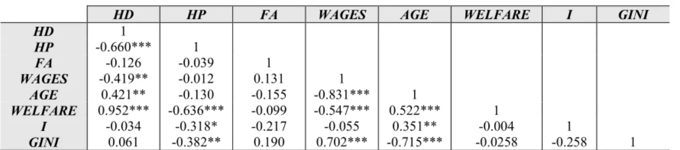
Table 3 – The correlation coefficients between variables
HD HP FA WAGES AGE WELFARE I GINI
HD 1 HP -0.660*** 1 FA -0.126 -0.039 1 WAGES -0.419** -0.012 0.131 1 AGE 0.421** -0.130 -0.155 -0.831*** 1 WELFARE 0.952*** -0.636*** -0.099 -0.547*** 0.522*** 1 I -0.034 -0.318* -0.217 -0.055 0.351** -0.004 1 GINI 0.061 -0.382** 0.190 0.702*** -0.715*** -0.0258 -0.258 1
Note: *** indicates statistical significance at 1% level, ** indicates statistical significance at 5% level and * indicates statistical significance at 10% level
As we can observe, four independent variables are statistically significant in terms of correlation with household debt, namely house prices, wages, age, and welfare. For this analysis, we need to take into account the fact that having lower correlations ensures that the model does not suffer multicollinearity problems.
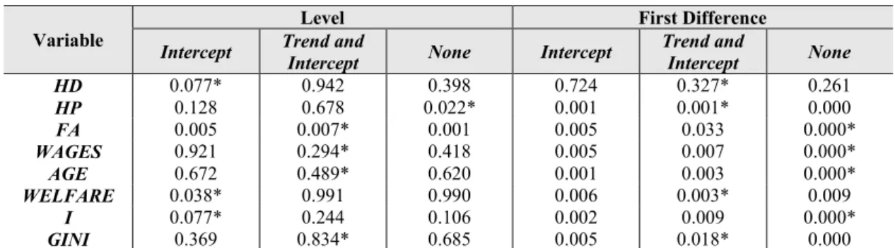
In order to select the more precise econometric methodology, we assess the existence of unit roots in all variables by applying the traditional augmented Dickey and Fuller (1979) (ADF) test and the Phillips and Perron (1998) (PP) test. The respective results are detailed in Table 4
21
and Table 5. The results of these two tests allow us to understand if the variables are stationary in levels (integrated of order zero) or stationary in first differences (integrated of order one). At the traditional significance levels, house prices, financial asset, and welfare are stationary in levels for both tests, in other words, they are integrated of order zero. The household debt is stationary only in levels by the ADF test. Wages only become stationary in first differences by the ADF test (they are integrated of order one), but stationary in levels by the PP test. Age and Gini coefficient only become stationary in first differences for both tests. The real long-term interest rate is stationary in levels by the ADF test but stationary in first differences by the PP test. As we can observe, we have a mixture of variables that are integrated of order zero and one.
Table 4 – P-values of the ADF test
Variable
Level First Difference
Intercept Trend and Intercept None Intercept Trend and Intercept None
HD 0.077* 0.942 0.398 0.724 0.327* 0.261 HP 0.128 0.678 0.022* 0.001 0.001* 0.000 FA 0.005 0.007* 0.001 0.005 0.033 0.000* WAGES 0.921 0.294* 0.418 0.005 0.007 0.000* AGE 0.672 0.489* 0.620 0.001 0.003 0.000* WELFARE 0.038* 0.991 0.990 0.006 0.003* 0.009 I 0.077* 0.244 0.106 0.002 0.009 0.000* GINI 0.369 0.834* 0.685 0.005 0.018* 0.000
Note: The lag lengths were selected automatically based on the AIC criteria and * indicates the exogenous variables included in the test according to the AIC criteria
Table 5 – P-values of the PP test
Variable
Level First Difference
Intercept Trend and Intercept None Intercept Trend and Intercept None
HD 0.419 1.000* 0.795 0.691 0.3341* 0.244 HP 0.134 0.771 0.023* 0.001 0.000 0.000* FA 0.005 0.026 0.001* 0.000 0.000 0.000* WAGES 0.901 0.003* 0.431 0.006 0.005 0.000* AGE 0.623 0.461* 0.613 0.001 0.003 0.000* WELFARE 0.038* 0.993 0.971 0.006 0.004* 0.001 I 0.172 0.424 0.101* 0.001 0.009 0.000* GINI 0.246 0.239 0.675* 0.005 0.002* 0.000
Note: * indicates the exogenous variables included in the test according to the AIC criteria
Given the results from ADF and PP test, in this dissertation, we will apply the autoregressive distributed lag (ARDL) estimator proposed by Pesaran (1997), Pesaran and Shin (1999) and Pesaran et al. (2001). According to Harris and Sollis (2003), ARDL estimator has three different aspects that justify its suitability in this specific case. Firstly, this estimator can be applied to variables of different orders, integrated of order zero and one. Secondly, this estimator is more
22
efficient even for small and finite samples. Thirdly, this estimator produces unbiased and consistent estimates, even in the long-term.
In the ARDL model, the dependent variable is explained by the lagged of itself and with both the contemporaneous and the lagged values of the independent variables. We can summarize this econometric methodology into four steps. Firstly, we need to analyze the number of lags that should be included in the estimates following the traditional information criteria. Secondly, we verify if there is a cointegration relationship between all the variables through the bounds test procedure proposed by Pesaran et al. (2001). Thirdly, we examine if our econometric model suffers from any econometric problems by conducting six diagnostic tests, namely autocorrelation, Ramsey’s RESET, normality, heteroscedasticity, the cumulative sum of recursive residuals (CUSUM) and the cumulative sum of squares of recursive residuals (CUSUMSQ). Fourthly, we present both long-term and short-term estimates for the Portuguese household debt.
23
Table 6 - Data used in the ARDL model
Year HD HP FA WAGES AGE WELFARE i GINI
1989 0,154 0,181 0,010 0,559 0,019 0,105 0,038 0,315 1990 0,152 0,150 -0,005 0,555 0,019 0,122 0,037 0,320 1991 0,163 0,194 -0,162 0,581 0,016 0,131 0,033 0,356 1992 0,174 0,124 -0,116 0,603 0,015 0,138 0,044 0,360 1993 0,219 0,013 0,145 0,606 0,015 0,151 0,042 0,363 1994 0,251 0,023 0,341 0,583 0,015 0,152 0,034 0,370 1995 0,283 0,015 -0,033 0,590 0,015 0,160 0,055 0,370 1996 0,328 0,016 0,156 0,601 0,014 0,166 0,060 0,360 1997 0,373 0,036 0,569 0,601 0,015 0,164 0,024 0,360 1998 0,440 0,045 0,584 0,601 0,015 0,168 0,010 0,370 1999 0,527 0,090 -0,085 0,597 0,016 0,172 0,013 0,360 2000 0,588 0,077 0,211 0,602 0,016 0,185 0,021 0,360 2001 0,634 0,054 -0,230 0,604 0,014 0,189 0,014 0,370 2002 0,673 0,006 -0,183 0,598 0,013 0,203 0,008 0,374 2003 0,716 0,011 -0,070 0,599 0,012 0,213 0,007 0,378 2004 0,758 0,006 0,275 0,586 0,012 0,217 0,017 0,378 2005 0,799 0,023 0,113 0,586 0,011 0,223 0,001 0,381 2006 0,839 0,021 0,296 0,572 0,018 0,220 0,007 0,377 2007 0,869 0,005 0,304 0,561 0,017 0,217 0,014 0,368 2008 0,890 -0,063 -0,251 0,567 0,018 0,222 0,027 0,358 2009 0,921 0,002 -0,163 0,576 0,020 0,245 0,031 0,354 2010 0,907 0,008 0,076 0,565 0,022 0,245 0,047 0,337 2011 0,905 -0,049 -0,045 0,555 0,023 0,244 0,105 0,342 2012 0,904 -0,071 -0,172 0,540 0,024 0,245 0,110 0,345 2013 0,861 -0,019 0,199 0,537 0,025 0,256 0,039 0,342 2014 0,817 0,042 0,069 0,527 0,025 0,251 0,030 0,345 2015 0,767 0,031 -0,079 0,516 0,025 0,240 0,004 0,340 2016 0,721 0,071 -0,028 0,514 0,021 0,237 0,014 0,339 2017 0,691 0,092 0,151 0,517 0,021 0,237 0,015 0,335 2018 0,669 0,103 0,096 0,521 0,020 0,226 0,004 0,321
Source: HD (household debt) and FA (financial assets) data are from FRED (Federal Reserve Bank of St. Louis).
HP (housing prices) and WELFARE (social spending) data are from OECD database. WAGES (adjusted wage share) and i (Real long-term interest rates) data are from AMECO. AGE (age dependency ratio) is from The World Bank. GINI (Gini coefficient) data is from 1989 (Rodrigues and Andrade,2013), since 1990 to 1993 from WIID – The World Income Inequality Database, since 1995 to 2018 from EUROSTAT and 2002 through linear interpolation.
24 4. RESULTS AND DISCUSSION
This section exhibits the estimates for Portuguese household debt. All results are produced with one lag according to the majority of the information criteria by lag (Table 7) and take into account that we are in the presence of annual data. Regarding the specification, we consider the constant and trend, because this seems to be more in line with the characteristics of the dependent variable (Figure A1 in the Appendix).
Table 7 – Values of the information criteria by lag
Portuguese Household
debt
Lag LR FPE AIC SC HQ
Total 0 1 278.164* n.a. 3.97e-30* 4.46e-26 -45.164* -35.670 -47.770* -35.293 -44.101* -35.552
Note: * indicates the optimal lag order selected by the respective criteria
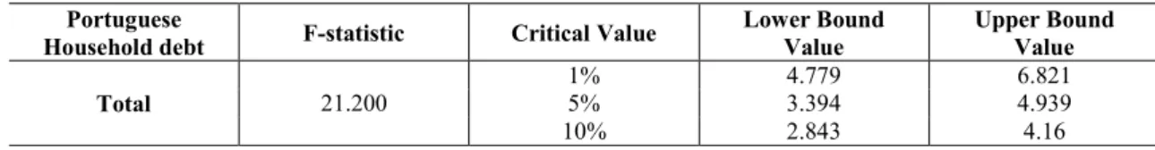
As already mentioned, after analysing the number of lags to be taken into account it is necessary to verify the existence of cointegrations relationship between all the variables by applying the bounds test procedure (Table 8). As we can observe, the computed F-statistics are above the upper bound critical value, which means that our variables are cointegrated.
Table 8 – Bounds test for cointegration analysis
Portuguese
Household debt F-statistic Critical Value Lower Bound Value Upper Bound Value
Total 21.200 1% 5% 4.779 3.394 6.821 4.939
10% 2.843 4.16
Then we performed four diagnostic tests (Table 9), the Breusch–Godfrey serial correlation LM test, Ramsey’s RESET test of functional form, Jarque–Bera test of normality and the ARCH test of homoscedasticity. According to the obtained results, it is possible to confirm that the ARDL model is well specified in their functional form due to the fact that the P-value achieved is higher than the significance level of 1%, 5% and 10%, the null hypothesis of no misspecification is not rejected. We exclude the presence of autocorrelation and confirm that our residuals are normal and homoscedastic. Also, we performed two stability diagnostic test, which are the cumulative sum of recursive residuals (CUSUM) and the cumulative sum of squares of recursive residuals (CUSUMSQ) (Figure A9 and Figure A10 in the Appendix). With the respective results, we confirm that the estimated coefficients are stable and verify the absence of structural breaks in our sample. All of these tests show that our model does not suffer
25
from any serious econometric problem, as a result we can proceed with the analysis of the long-term estimates (Table 10) and short-long-term estimates (Table 11).
Table 9 – Diagnostic tests for ARDL estimates
Household debt Test F-Statistic P-value
Total
Autocorrelation 2.018 0.179
Ramsey’s RESET 0.060 0.810
Normality 0.720 0.698
Heterocedasticity 1.163 0.391
Note: Autocorrelation tests were conducted with 1 lag and Ramsey’s RESET tests were performed with 1 fitted term, albeit results do not change if we had used more lags and more fitted terms, respectively
In the long-term only the wages, welfare and real long-term interest rate are statistically significant at the traditional significance levels. An increase of state spending on social assistance implies a rise of household debt in Portugal. On the other hand, a rise of wages and an increase of real long-term interest rate makes cause exert a negative effect on Portuguese household debt. The welfare and wages variables were tested directly only by Stockhammer and Moore (2018), however, the results obtained are inconsistent with them. The authors did not find any evidence for long-run effects for both hypotheses. In relation to the real long-term interest rate, the result confirming the previous empirical findings (Farinha and Noorali, 2004; Castro, 2006; Morais, 2013; Stockhammer and Wildauer, 2017) with exception of Stockammer and Moore (2018) study. Stockammer and Moore (2018) used the real short-term interest rate as a proxy variable for the low interest rate hypothesis, consequently, the results may be different due to the fact that the data is not the same.
Table 10 – The long-term estimates of Portuguese Household debt (1989-2018)
Variable Coefficient Standard errors t-statistics
HPt -0.024 0.861 -0.027 FAt -0.341 0.254 -1.339 WAGESt -12.256** 5.502 -2.228 AGEt 18.830 16.533 1.139 WELFAREt 20.359*** 5.316 3.893 it -2.751* 1.555 -1.770 GINIt -4.560 3.387 -1.346
Note: *** indicates statistical significance at 1% level, ** indicates statistical significance at 5% level and * indicates statistical significance at 10% level
In the short-term, it is important to highlight three points. Firstly, only two variables are statistically significant, namely house prices and wages. In the short-term, rising real estate prices and an increase in wages makes cause an increase in Portuguese household debt. The house prices variable have a statistically effects at 1% level. This result is supported by studies performed by Stockhammer and Wildauer (2017) and Stockhammer and Moore (2018). The authors also find strong evidence for the house prices hypothesis. The wages variable have
26
statistically effects at 5% level. As expected, the effect for this variable for short-term is positive due to the fact that for long-term the effect it is the opposite (negative effect). The result obtained is inconsistent from Stockhammer and Moore (2018) finding. Secondly, the model describes reasonably well the Portuguese household debt given the high R-squared and Adjusted R-squared values, respectively. Thirdly, the coefficient of the error correction terms is strongly statistically significant but have an unexpected and slightly positive sign. This result confirm the stability of the model and shows the divergence to the long-term equilibrium if there is any shock in the short-term. This should not compromise the reliability of our estimates, because we already conclude that our model passed in all diagnostic tests.
Table 11 – The short-term estimates of Portuguese household debt (1989-2018)
Variable Coefficient Standard Error T-statistic
C -0.599*** 0.041 -14.519 @TREND 0.008*** 0.001 11.360 ∆HPt 0.128*** 0.041 3.1312 ∆FAt 0.005 0.006 0.800 ∆WAGESt 0.441** 0.184 2.397 ∆AGEt 0.317 0.900 0.353 ∆WELFAREt -0.412 0.259 -1.589 ECTt-1 0.099*** 0.006 15.950
R-squared = 0.962 Adjusted R-squared = 0.949
Note: ∆ is the operator of the first differences, *** indicates statistical significance at 1% level, ** indicates statistical significance at 5% level and * indicates statistical significance at 10% level
Despite the differences in sample and method used in the identified literature, in a global overview, the dissertation find a positive and significant impact mainly of house prices (Farinha and Noorali , 2004; Farinha, 2007; Stockhammer and Wildauer, 2017; Stockhammer and Moore, 2018) and low interest rate on household indebtedness (Farinha and Noorali, 2004; Castro, 2006; Morais, 2013; Stockhammer and Wildauer, 2017). The main difference obtained in this dissertation ainst the conclusions in the identified literature are related to the falling wages and welfare retrenchment hypothesis. As already mentioned, these two hypothesis were only tested by Stockhammer and Moore (2018). Regarding falling wages hypothesis, Stockhammer and Moore (2018) found some evidence for the rejection of the hypothesis in the short-run and no evidence for long-run effects. Their result is inconsistent with the results obtained through the ADRL model in this dissertation. Concerning welfare retrenchment, Stockhammer and Moore (2018) rejected this hypothesis, because the authors did not find evidence for long and short-run effects.
27
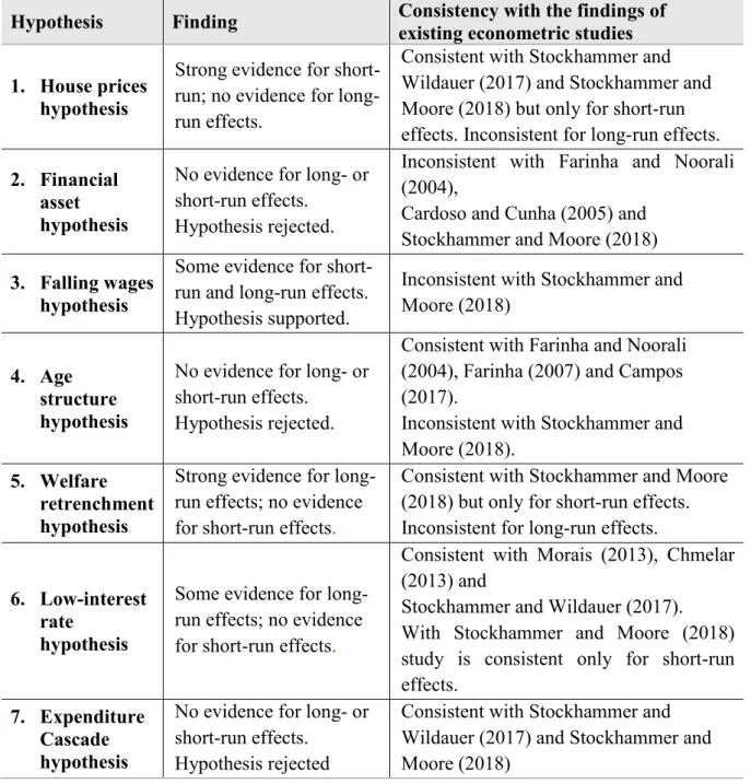
Table 12 – Comparison of results with the findings of existing econometric studies
Hypothesis Finding Consistency with the findings of existing econometric studies 1. House prices
hypothesis
Strong evidence for short-run; no evidence for long-run effects.
Consistent with Stockhammer and Wildauer (2017) and Stockhammer and Moore (2018) but only for short-run effects. Inconsistent for long-run effects. 2. Financial
asset hypothesis
No evidence for long- or short-run effects.
Hypothesis rejected.
Inconsistent with Farinha and Noorali (2004),
Cardoso and Cunha (2005) and Stockhammer and Moore (2018) 3. Falling wages
hypothesis
Some evidence for short-run and long-short-run effects. Hypothesis supported.
Inconsistent with Stockhammer and Moore (2018)
4. Age structure hypothesis
No evidence for long- or short-run effects.
Hypothesis rejected.
Consistent with Farinha and Noorali (2004), Farinha (2007) and Campos (2017).
Inconsistent with Stockhammer and Moore (2018).
5. Welfare retrenchment hypothesis
Strong evidence for long-run effects; no evidence for short-run effects.
Consistent with Stockhammer and Moore (2018) but only for short-run effects. Inconsistent for long-run effects.
6. Low-interest rate
hypothesis
Some evidence for long-run effects; no evidence for short-run effects.
Consistent with Morais (2013), Chmelar (2013) and
Stockhammer and Wildauer (2017). With Stockhammer and Moore (2018) study is consistent only for short-run effects.
7. Expenditure Cascade hypothesis
No evidence for long- or short-run effects.
Hypothesis rejected
Consistent with Stockhammer and Wildauer (2017) and Stockhammer and Moore (2018)
Summing up, it is possible to confirm that house prices and wages are the main determinants of household debt in Portugal in the short-term. Concerning to the long-term, wages, welfare retrenchment and the interest rate are the mains determinants of household debt in Portugal. The only hypothesis which is consistent either for short and long term is the falling wages. The results show that wages are the most robust determinant both in the long-term and in the short-term. In the long-term a decrease in wages causes an increase in Portuguese household debt. In short-term, an increase in wages makes cause an increase on Portuguese household debt. Due
28
to wage cuts, the Portuguese households take out credit to maintain the same level of consumption as in the past.
29 5. CONCLUSIONS
This dissertation investigates the determinants of household debt in Portugal by performing a time series econometric analysis from the beginning of the year of 1989 until the end of the year 2018. Was estimated a household debt equation using seven independent variables, namely house prices, financial asset, welfare, wages, age, real long-term interest rate, and Gini coefficient. These variables were chosen based on those already used in the identified literature on household indebtedness. We have a mixture of variables that are stationary in levels and stationary in first differences, which implied the utilization of the ARDL econometric methodology.
The findings show that wages is the most robust determinant of household indebtedness both in the long-term and in the short-term. In the long-term a decrease in wages causes an increase in Portuguese household debt, instead of for short-term, an increase in wages causes an increase in Portuguese household debt. This result is inconsistent with Stockhammer and Moore (2018) study, the only authors that studied this hypothesis. However, this hypothesis is not the only identified determinant of household debt in Portugal. Also, for short-term period, the house prices have a strong impact on the Portuguese household debt. This result is in accordance with other empirical studies about this theme (Farinha and Noorali, 2004; Farinha, 2007; Stockhammer and Wildauer, 2017; Stockhammer and Moore, 2018), which confirmed that this variable is positive and have a significant impact in household indebtedness. In relation to the long-term, as well, low interest rate and welfare retrenchment are the determinants of household debt. The results regarding low interest rate are in line with the results of other empirical studies about this subject (Farinha and Noorali, 2004; Castro, 2006; Morais, 2013; Stockhammer and Wildauer, 2017).
One of the biggest constraints was finding the necessary information for all variables from 1989 to 2018. Unfortunately, the credit supply hypothesis could not be tested due to the difficulty of obtaining accurate data on the total credit granted to households for the pretended period. As previously mentioned, it was important to test this hypothesis since, to understand whether the credit supply will be attractive and if there is no proper financial regulation, this will allows households to take on more debt. Additionally, the fact that the interest rate is at historic lows makes credit much more desirable. Stockhammer and Moore (2018) also failed to test this hypothesis.
30
Despite the limitations, it is important to highlight the fact that the findings on this dissertation have impacts both for economic research and for economic policy. In terms of research, in the identified literature regarding the Portuguese household indebtedness, none of the studies addressed in the same study seven hypothesis together. Also, some concepts were not studied for Portugal such as the welfare retrenchment and expenditure cascade. In terms of economic policy, the results reinforce all the conclusions achieved so far and the ongoing debates on macroprudential policies. The fact that the interest rate remains low will increasingly encourage household consumption and in turn, increase their indebtedness. It is important to act quickly and create more controls on credit supply, as well as creating rules in the real estate market, in order to avoid other financial crises and encourage sustainable growth in the country. As Chmelar (2013) mentioned, the debt overhang and the contraction of demand has been just as important an impediment to the return of growth. Stockhammer and Moore (2018) stated that unsustainable levels of household debt are known to threaten financial and macroeconomic stability central banks should act against debt and real estate booms.
Furthermore, future analysis on this topic should focus on the empirical assessment of the causes of rising house prices as well as the respective consequences of such increase. Given that there were no studies on the hypotheses of welfare retrenchment and falling wage for Portugal, it would be important to conduct more focused studies on these two variables in order to reinforce and corroborate the results presented here.
31 6. REFERENCES
Alves, J and Pereira, R (2017), The Portuguese Households’ Indebtedness, working paper, ISEG – Lisbon school of economics & management
Bank of Portugal (2018), Financial Stability Report of June 2018
Browning, M., & Crossley, T.F. (2001), The lifecycle model of consumption and saving.
Campos, Cláudio (2017), Determinants of the Portuguese families’ level of over-indebtedness, Management master dissertation, NOVA – School of Business & Economics
Cardoso, F. and Cunha, V (2005). ‘Household wealth in Portugal: 1980-2004’. Economic Research Department, Bank of Portugal
Castro, G. L. (2006), “Consumption, Disposable Income and Liquidity Constraints”, Economic Bulletin, Bank of Portugal, pp.75-84
Castro, G. L. (2007), ‘The Wealth Effect on Consumption in the Portuguese Economy’. Economic Bulletin Winter, Bank of Portugal, pp. 37-55
Chmelar, Ales (2013), "Household Debt and the European Crisis", paper presented at the ECRI Conference, 16 May 2013, Brussels
Colletta, Massimo et al (2018), “The Household Debt in OECD Countries: The Role of Supply-Side and Demand-Supply-Side Factors”, Sringer Nature, (Online)
Costa, S. and Farinha, L. (2012), “Households’ indebtedness: a microeconomic analysis based on the results of the households’ financial and consumption survey”, Financial Stability Report 2012, Bank of Portugal, pp. 133-157
Costa, Sónia (2012), “Households’ default probability: an analysis based on the results of the HFCS”, Financial Stability Report, November 2012, Bank of Portugal, pp. 97-110
Dickey, D. A. and Fuller, W. A. 1979. ‘Distribution of the Estimators for Autoregressive Time Series with a Unit Root’. Journal of the America Statistical Association. 74 (366): 427-431. Farinha, Luísa (2007), “Indebtedndess of Portuguese Households: recent evidence based on the
household wealth survey 2006-2007”, Financial Stability Report 2007, Bank of Portugal, pp. 129-152
Farinha, Luísa 2008. ‘Wealth Effects on Consumption in Portugal: A Microeconometric Approach’. Financial Stability Report 2008, Bank of Portugal
Farinha, Luísa and Nooralli, Sara (2004), “Indebtedness and Wealth of Portuguese Households”, Finacial Stability Report – 2004, pp.131-143
Harris, H. and Sollis, R. (2003), Applied Time Series Modelling and Forecasting. Wiley, West Sussex.
32
Morais, Lavínia (2013), Determinantes e efeitos do endividamento das famílias em Portugal, Accounting and Finance master dissertation, Bragança, Instituto Politécnico de Bragança Pesaran, M. H. (1997), ‘The Role of Economic Theory in Modelling the Long Run’. Economic
Journal. 107 (1): 178-191.
Pesaran, M. H. and Shin, Y. (1999), ‘An Autoregressive Distributed-Lag Modelling Approach to Cointegration Analysis’. In Strøm, S. (ed.): Econometrics and Economic Theory in the Twentieth Century: The Ragnar Frisch Centennial Symposium. Cambridge: Cambridge University Press.
Pesaran, M. H.; Shin, Y.; and Smith, R. J. (2001). ‘Bounds Testing Approaches to The Analysis of Level Relationships’. Journal of Applied Econometrics. 16 (1): 289-326.
Petra Gerlach-Kristen & Seán Lyons (2017): “Determinants of mortgage arrears in Europe: evidence from household microdata”, International Journal of Housing Policy, (Online) Phillips, P. C. B. and Perron, P. (1998). ‘Testing for a Unit Root in Time Series Regression’.
Biometrika. 75 (2): 335-346.
Rodrigues, C. F. and Andrade, I. (2013), Growing Inequalities and Their Impacts in Portugal, working paper
Sousa, R. M. (2008). “Financial Wealth, Housing Wealth, and Consumption”. International Research Journal of Finance and Economics, 19: 167-191
Stockhammer, E. and Moore, G. L. (2018), The drivers of household indebtedness re-considered: an empiricial evoluation of competing arguments on the macroeconomic determinants of household indebtedness in OECD countries, working paper 1803, Post-keynesian economics society
Stockhammer, E. and Wildauer, R. (2017), Expenditure Cascades, Low Interest Rates or Property Booms? Determinants of Household Debt in OECD Countries, working paper 1710, Post Keynesian Economics Study Group
Wildauer, Rafael (2017), “Determinants of Household Borrowing in the United States and a Panel of OECD Countries Prior to the Financial Crisis of 2007/2008”, Department of Economics Kingston University