Repositório ISCTE-IUL
Deposited in Repositório ISCTE-IUL:2019-03-22
Deposited version:
Post-print
Peer-review status of attached file:
Peer-reviewed
Citation for published item:
Martins, L. F., Gan, Y. & Ferreira-Lopes, A. (2017). An empirical analysis of the influence of macroeconomic determinants on World tourism demand. Tourism Management. 61, 248-260
Further information on publisher's website:
10.1016/j.tourman.2017.01.008
Publisher's copyright statement:
This is the peer reviewed version of the following article: Martins, L. F., Gan, Y. & Ferreira-Lopes, A. (2017). An empirical analysis of the influence of macroeconomic determinants on World tourism demand. Tourism Management. 61, 248-260, which has been published in final form at
https://dx.doi.org/10.1016/j.tourman.2017.01.008. This article may be used for non-commercial purposes in accordance with the Publisher's Terms and Conditions for self-archiving.
Use policy
Creative Commons CC BY 4.0
The full-text may be used and/or reproduced, and given to third parties in any format or medium, without prior permission or charge, for personal research or study, educational, or not-for-profit purposes provided that:
• a full bibliographic reference is made to the original source • a link is made to the metadata record in the Repository • the full-text is not changed in any way
The full-text must not be sold in any format or medium without the formal permission of the copyright holders.
An Empirical Analysis of the In‡uence of Macroeconomic
Determinants on World Tourism Demand
Luís Filipe Martins
ISCTE-IUL, BRU-IUL and CIMS-University of Surrey
Yi Gan AJEPC Alexandra Ferreira-Lopes
ISCTE-IUL, BRU-IUL, and CEFAGE-UBI
This version: 6 August, 2015
Abstract
This paper considers three econometric models to determine the relationship between macroeconomic variables and tourism demand. Tourism demand is measured by the inbound visitor’s population and also by on-the-ground expenditures. Macroeconomic determinants include the exchange rate, the relative domestic prices, and the World GDP per capita. The database is an unbalanced panel of 218 countries over the period 1995-2012. There is evidence that an increase in the World’s GDP per capita, a depreciation of the national currency, and a decline of relative domestic prices do help boosting the number of arrivals and the correspondent expenditure level. The World’s GDP per capita is more relevant when explaining arrivals, but relative prices become more important when we use expenditures as the proxy for tourism demand. In particular, we cannot reject the hypothesis of a relative prices unitary elasticity of expenditures. Additionally, we have also partitioned our data by income level and by continent. Results are robust in the …rst partition, but less robust in the second, although the main conclusions still hold.
JEL Classi…cation: C23, L83.
Keywords: Tourism demand, exchange rate, relative domestic prices, world income, panel data model, Poisson panel data model.
We thank Tiago Sequeira for helpful comments. The usual disclaimer applies. The corresponding author is Luis Filipe Martins, Email: [email protected]; URL: http://home.iscte-iul.pt/~lfsm/
1
Introduction
As one of the important industries of the tertiary sector, the tourism industry has been develop-ing rapidly in the last decades and contributdevelop-ing signi…cantly for economic growth, especially in tourism-intensive countries. And the demand for tourism continues to rise, since the transports sector has also been signi…cantly developing. Consumers have more means of transportation at their disposal, which are faster and cheaper, allowing them to choose over more destinations. With this growing trend in the travel and tourism industries, …rms can take the chance to in-crease their income, by attracting more customers, if they e¤ectively forecast their demand and allocate resources in a reasonable way. The macroeconomic determinants of tourism demand, at the world level, are the focus of our work. We will focus on three macroeconomic determinants of tourism demand - the nominal exchange rate, relative prices and world income per capita. We based our choices on the results draw from previous literature, which we present in the next section.
The choice to include the nominal exchange rate as a determinant is obvious, since a de-preciation of a given currency relative to others, can increase the demand for tourism, hence domestic prices become relatively cheaper than import prices. A substantial amount of previous research focused on analyzing the relationship between this variable and tourism demand and found a somewhat robust and positive relationship between the two. We have also chosen to include relative prices, i.e., the ratio of domestic prices over foreign prices (in our case, the con-sumer price index of the USA is the proxy chosen for foreign prices) as an important explanatory variable. This variable measures the cost of living in the country in comparison with the USA, so it measures the purchasing power in the visited country. The expected sign of this variable is negative, since the higher the purchasing power of the visited country vis-à-vis the USA, the lower the probability of having many tourists. The literature has focused its attention mostly on the consumer price level (CPI) of the country and not much on the comparison between the CPI of the country and that of the rest of the World. We think a comparison of purchasing power is more important for consumer (tourist) decision than a mere introduction of the price level of the country itself. Additionally, in the tourism literature, income or economic growth has been playing an important role, either as a source or as consequence of tourism demand. Since in our work we are dealing with a panel of 218 countries, we consider the World GDP per capita, i.e., the average of World income, as one of our determinants for tourism demand, because it re‡ects
the global economic environment and wealth. The expected sign for this variable is positive, since we expect that an increase in average World income increases tourism demand.
We model tourism demand, our variable of interest, from two perspectives - value and quan-tity. From the value perspective we use on-the-ground expenditures. From the quantity per-spective we use arrivals to the destination country as our variable. Besides distinguishing the determinants for tourism value and quantity, we use a log-log model speci…cation so that the measurement units of the macroeconomic variables will not matter in ranking the importance of these in explaining tourism demand. Based on panel methods for count (Poisson regression) and real-valued data, we conclude that the World’s GDP per capita is more signi…cant when explaining arrivals and relative prices is more relevant when we use expenditures as the proxy for tourism demand.
Additionally, many of the studies so far applied the data for a speci…c country, region, or small group of countries, which may ignore the heterogeneity among destinations and also World-wide e¤ects. Hence, these studies lack universality, making it di¢ cult to apply their results and conclusions to a larger extent. To increase the scope of the literature, our work is going to analyze a panel of 218 economies, spread throughout all continents, thus covering the entire world. Our micro panel covers the period between 1995 and 2012 and it is found that the number of arrivals grew 1.2% per year whereas relative expenditures declined at a rate of about 2% per year.
Finally, we have also partitioned our data by income level and by continent to check whether the relative importance of each macroeconomic variable is indi¤erent to these two world aspects. Results are robust in the …rst partition, but less robust in the second, although the main con-clusions still hold. Quite interesting, the results suggest that the world income is relevant to high income countries and the relative prices to low and middle income countries and that the relative prices have a much lower impact in Europe, when compared to other continents.
This work is structured as follows. In Section 2 we perform a literature review of the works closely related to our topic of study and that motivates the choice we make for the macroeconomic variables. Section 3 describes the empirical approach, i.e., data and methodology, Section 4 discusses the results and Section 5 analyses two extensions: income levels and continents. Finally, Section 6 concludes.
2
Literature Review
In this section we analyze the most relevant literature related with the macroeconomic determi-nants, which we use in our study as explanatory variables for tourism demand.
One of the macroeconomic variables that we use as a possible determinant of tourism demand is (World) income per capita. Previous literature has mainly used economic growth, i.e., the growth rate of GDP, as the variable of interest, and not the level or average income. This previous literature was mainly concerned about the direction of causality between tourism and growth. Additionally, most of the literature explores the in‡uence of tourism on economic growth and few explore the reverse causality. Some of the studies presented below also use the nominal exchange rate and some proxy for prices as explanatory variables, but not in the same context as we do.
Sequeira and Campos (2007) investigated the causality between international travelling and economic development. The authors used variables such as the degree of openness, the investment-output ratio, tourist arrivals per head of population, tourism receipts in % of ex-ports, the black market premium, real GDP, secondary male enrolment, and the government consumption-output ratio, from 1980 to 1999, obtained from the Penn World Tables and the World Bank. Using panel data regression (with …xed or random e¤ects), they reached the fol-lowing conclusions: the chosen tourism variables are not closely correlated with the economic boom, regardless of tourism-specialized countries or a wider range of other countries. In latter research, Sequeira and Nunes (2008a) introduced three additional variables: secondary years of schooling above 25 years, life expectancy, and international country risk guide, using the corrected Least Square Dummy Variables (LSDVC) or the …xed E¤ects (FE) approach and the Generalized Method of Moments (GMM) estimator. Results show that poor countries can pro…t from specializing in tourism, not only in tourist receipts, but also in consumption, which con-tributes to the development of the economy. On the other hand, small countries are bene…ting less from the specialization in the tourism industry.
According to Odhiambo (2011), with data for 1980-2008, using the Autoregressive Distrib-uted Lag (ARDL) bounds testing approach, unlike most of the previous research, in Tanzania, tourism development leads to more economic growth in the short term, however, in the long run, growth-led tourism plays the important role. Meanwhile, statistical analysis also indicates that in the short run, there are bidirectional relationships between exchange rate and tourism
development, and between exchange rate and economic growth. Research for Mediterranean countries shows similar results. Dritsakis (2012), using the method of cointegration analysis and data for real GDP per capita, real tourism receipts per capita and real e¤ective exchange rate, in the period 1980-2007, reveals that tourism development is closely related to GDP in seven Mediterranean countries: Greece, Turkey, Cyprus, Spain, France, Italy, and Tunisia. Further-more, the author suggests that governments should assist the tourism industry to grow as much as possible.
Harvey et al. (2013) applied the bounds testing approach to cointegration and an error-correction model to a linear-log equation, with data from the World Bank and the International Financial Statistics (IFS) of the International Monetary Fund (IMF) (1995-2010), using vari-ables like the real GDP, annual international tourist arrivals, the nominal exchange rate, and real exchange rate. The empirical evidence from the Philippines indicated that not only short run but long run growth will bene…t from tourism development. As a member of the Brunei-Indonesia-Malaysia-Philippines - East ASEAN Growth Area (BIMP-EAGA), Philippines imple-mented some measurements to boost economic cooperation, including tourism relations, which contributed to economic development. The same thing happened in Jamaica. By examining the causal relationship between …nancial development and tourism industry, Ghartey (2013) con…rmed that tourism arrivals and expenditure lead to economic growth, by introducing the consumer price index (CPI), the GDP and tourism arrivals between 1963 and 2008, into a Vec-tor AuVec-toregressive (VAR) model, both in the long and in the short term. In 1986, due to the depreciation of the domestic currency, tourism expenditure ascended, being conducive to more economic growth in the country.
The exchange rate and prices are also considered as vital variables of explanation for tourism demand, and a strand of research is committed to clarify the relationship among them.
Cheng et al. (2013a, b) introduced the Structural Vector Autoregressive model (SVAR) to study the relationship between tourism revenues (exports) and tourism spending (imports). This paper illustrates the exchange rate e¤ects on US tourism trade balance, using the SVAR model, using data from 1973 to 2007, for the exchange rate, tourism exports and imports. There is no evidence of a J-curve behavior (The J-curve behavior means that in the short run, currency depreciation leads to a trade balance de…cit, instead of a surplus, like it is expected) of the US tourism trade balance with the US dollar depreciation, and a unit elastic e¤ect hypothesis of US tourism trade balance was raised. Export revenue is …nitely sensitive to the exchange rate
only. In these two works the nominal exchange rate was the only variable of interest that was related to tourism.
The following work only considers the impact of prices on tourism. The impact of prices on the number of tourists is di¤erent depending on the departing countries. The demand varia-tion in tourism demand of New Zealand was estimated by Schi¤ and Becken (2011). The log-log speci…cation was chosen, which gives a direct elasticity estimate. Elasticities for not only interna-tional visitor arrivals but on-the-ground expenditure per arrival are estimated for each segment. Analyzing the annual data for arrivals and the consumption from 16 countries (1997-2007), the authors concluded that the traditional segments, like the USA and Australia, were less price sensitive, while the Asian markets are relatively more sensitive to prices. Since the price is one of the critical components for tourists’decision, the inspection of price competitiveness relatively to the exchange rate and internal in‡ation should be consider.
The following works relate both exchange rates and prices with tourism, and in some of these works income or growth is also used as an explanatory variable. Lee et al. (1996) estimated the demand from inbound tourism expenditures for South Korea from eight tourists-originating countries. The annual time series data is used in this study for the period between 1970 and 1989. The income of tourists, prices and other special factors such as political unrest, economic recessions and mega events (e.g., World Expo) are considered as major determinants. The log-log speci…cation is applied, estimated by Ordinary Least Squares (OLS). Income has positive and signi…cant in‡uence, while prices have negative and signi…cant impact, and the exchange rates have positive signs for all the countries except for the UK. But dummy variables like mega events are generally insigni…cant.
Dwyer and Forsyth (2002) made a comparison of price competitiveness among Australia and 13 chosen destination countries. The article discusses the tourism price competitiveness relative to the exchange rate and domestic in‡ation of the destinations, using Australia as the base case. The appreciation of the exchange rate and the in‡ation rate jointly determine the price competitiveness. With the devaluation of the Australia dollar from 1985 to 1997, all 13 countries raised the price competitiveness compared with Australia. And the countries which kept relatively lower in‡ation rates greater enlarged their competitive advantage. In the case of Taiwan, while the e¤ects of relative prices and exchange rate volatility tend to be di¤erent, the exchange rate typically has the expected negative impact on tourist arrivals to Taiwan. Whereas exchange rate volatility can have positive or negative e¤ects on tourist arrivals to
Taiwan, depending on the source of the international tourists (Chang and Mcaleer, 2012). The authors use daily data on exchange rates and its volatility; arrivals of tourism to Taiwan from Japan, the USA, and the Rest of the World from 1 January 1990 to 31 December 2008. To capture the approximate long-memory properties in the tourist arrivals series, the heterogeneous autoregressive model is applied.
Saayman and Saayman (2013) studied the impact of exchange rate volatility on tourism in South Africa. It is assumed that the volatility of the South African Rand, the local currency (the ZAR) has an important impact on both visitors’ spending and arrivals only from 2000 onwards, when the South African currency was permitted to free ‡oat. Volatility is modeled using a GARCH model, while the in‡uence thereof on tourism is modeled using an autoregres-sive distributed lag model (ADL) and a bounds test approach. Using quarterly data for the period between 2003 and 2010 for average spending, tourism arrivals, real GDP, CPI, nominal exchange rate, and the main sources (countries) of intercontinental arrivals, respectively Aus-tralia, Germany, the UK, the USA, France, Brazil, and China. The authors found that increased currency volatility is associated with an increase in on-the-ground expenditure in most of the countries, respectively China, Germany, the USA, and Brazil, while Australian tourists tend to take smaller risks, spending less when volatility increases. In terms of arrivals, most of the countries showed risk aversion behavior, at the exception of China. Due to increased currency volatility, arrivals declined. Last but not least, in the long term, spending would be in‡uenced more than arrivals.
Chao et al. (2013) examined how currency depreciation a¤ects the prices of inbound tourism, illustrating that the exchange rate has a dominant e¤ect in the amount of tourists that a country receives. Also, the e¤ect of rising domestic price in‡ation can be passed through to foreigners, via consumption, while tourists are staying in the country. Consequently, the depreciation of the domestic currency may harm the revenue of inbound tourism. Currency volatility a¤ects not only the visitor’s expenditure but also arrivals, and in the long run, revenues will be in‡u-enced even more. Another example using German tourists who travel to Turkey, also showed that exchange rates are signi…cant determinants of tourism demand (De Vita and Kyaw, 2013). The authors collected observations on Turkey’s tourist arrivals from Germany from 1996 to 2009, at quarterly frequency, to analyze its relationship with exchange rates (the authors tested alternative exchange rates volatility measures), using Generalized Autoregressive Conditional Heteroscedasticity (GARCH) speci…cation and a variance volatility measure. To sum up,
ex-change rates are signi…cant determinants of tourism demand. Secondly, the exex-change rate and a relative price proxy should not enter the tourism demand model separately, but rather be combined as an exchange rate adjusted e¤ective price variable.
See also De Vita (2014) on the impact of exchange rate regimes on international tourism ‡ows using a panel of 27 countries over the period 1980 to 2011, Kiliç and Bayar (2014) for an empirical study for the Turkish tourism industry, Chen et al. (2015) for the impact of some macroeconomic variables (the growth rate of GDP, the in‡ation rate) on Taiwan’s tourism market cycle, and Salman et al. (2011) for the impact of the exchange rate, the CPI, and income on Sweden’s inbound tourism demand.
This work will also focus on the relationship between exchange rates, prices, income, and the number and volume of expenditures of inbound tourists, but taking into account a panel of 218 countries between 1995 and 2012, allowing to reach robust conclusions, about the relevance of these macroeconomic variables as determinants for tourism demand. These three macroeconomic variables will be jointly combined in econometric speci…cations.
3
Empirical Approach
In this section we describe the data, as well as the econometric methodology that we use in our estimations.
3.1 Data
The sample of the variables used in the models was taken from several data sources.
To measure tourism demand we use the countries’number of arrivals (inbound visitors) and the on-the-ground expenditure level, between 1995 and 2012, collected from the World Tourism Organization. There are four approaches to compile the tourism arrivals, namely the arrivals of non-resident tourists at national borders (TF), arrivals of non-resident visitors at national borders (VF), arrivals of non-resident tourists in hotels and similar establishments (THS) and arrivals of non-resident tourists in all types of accommodation establishments (TCE). In this paper, we have used the criteria TF and VF, which give us a more precise …gure for the number of tourists’arrivals, so countries for which these criteria are not observed were eliminated from our database. For the volume of expenditures, the data compiled by the WTO comes from the International Monetary Fund (IMF). We end up with a database of 218 countries.
The nominal exchange rate (XR) is de…ned with respect to the US dollar, the dominant vehicle currency in the international monetary system. For the Gross Domestic Product (GDP) we use the expenditure-side real GDP at chained Purchasing Power Parity (PPP), to allow for inter-country comparisons (RGDPE). We have also obtained data for the population (POP), so we can transform the variables in per capita terms, if necessary. These three variables were obtained from the Penn World Tables versions 7.1 and 8.0.
The consumer price index (CPI) measures the price level of a consumer basket of goods and services purchased by households. The collected data for CPI is from 1995 to 2012, and its source is the World Bank. Instead of directly using the domestic CPI as a covariate in the models, we use the relative domestic prices, as it is more appropriate for the tourist’s perspective, and it is with respect to the US price level (RP), this last one used as a proxy for the "World CPI".
The World Gross Domestic Product (World GDP), at current prices, is also introduced as one of the key determinants of tourism demand. The statistics from 1995-2012 were gathered from the IMF, World Economic Outlook Database.
The measurement units of each variable are listed in Table 1 below.
[TABLE 1 ABOUT HERE]
As a whole, the dataset we use is a signi…cant micro unbalanced panel. It covers essentially all countries in the world, although for some of them a few variables of the models are not observed for the entire time period. Nevertheless, the total number of observations used to estimate the tourism demand models is clearly meaningful: it ranges from a total of 1606 to 2190 data points.
3.2 Methodology
We specify three di¤erent econometric models for tourism demand as a function of the macro-economic variables exchange rate (XR), relative prices (RP), and the World GDP (WGDP). We measure tourism demand either in terms of quantity (tourism arrivals) or in terms of price (tourism expenditures). For the latter, tourism demand is proxied by Real Expenditures per Arrivals or Real Expenditures per Domestic GDP.1 That is, instead of the total level of
expen-ditures, we model how much a tourist spends on average in a journey or the weight tourism’s expenditures have relatively to the GDP of each economy.
1
Besides modeling the number of arrivals, we also have estimations for the number of arrivals relatively to the domestic populations (Arrivals/Pop). In this paper, we do not present the results for Arrivals/Pop because the estimated coe¢ cients associated to the covariates XR and RP have the wrong expected signs (negative for XR and positive for RP). Nevertheless, it is worth mentioning that Arrivals/Pop has experienced an estimated increase of 3% a year, something that con…rms that tourism has grown as an industry in the past years.
These three models were estimated taking log-log speci…cations, so that the coe¢ cients are interpreted as elasticities and thus independent of the measurement units chosen for the variables. Additionally, we can also rank the three explanatory macroeconomic variables to see which has the highest importance for tourism demand, in terms of elasticity.
The models contain two more features in order to best capture the main drivers of tourism demand. To account for time-e¤ects, we add a deterministic linear time trend to the models. We have 18 years of observations in the sample and, therefore, it is plausible that tourism demand in the world has been following a deterministic path over time. Since we have a micro-type of panel (the number of years, T = 18, is "small" relatively to the number of countries, n = 218) with unbalanced data, we do not consider dynamic panel models where the lagged dependent variable is included in the list of regressors of the model.
The second feature of the models is the existence of a component that captures all unob-servable country-speci…c characteristics that also helps determining the tourism demand and which is assumed to be time-invariant such as the risk of the country (see Sequeira and Nunes, 2008b, for example). Note that, by assuming that these individual e¤ects are unobserved, we do not have problems of mismeasurement of variables and the associated bias that it introduces in the estimation stage. Following the standard approach in panel data regression models, we test for the existence of country-speci…c e¤ects and, in the case of its presence, we further test for random e¤ects against …xed e¤ects.
The number of arrivals is modeled by means of a panel Poisson regression for count dependent variable because Arrivals takes nonnegative integer values for all countries and years:
it= E (Arrivalsitjxit; i) = iexp x0it exp i+ x0it ; i = 1; :::; n; t = 1; :::; T; (1)
where E ( j ) is the conditional expectation, xit includes XRit; RPit; W GDPit (all in logs) and
controls for individual country-e¤ects. Taking logs,
log it= log E (Arrivalsitjxit; i) = i+ 1log XRit+ 2log RPit+ 3log W GDPit+ 4t: (2)
The values of j; j = 1; 2; 3 shall be interpreted as point elasticities whereas 4 is the percentage change of E (Arrivalsitjxit; i) per year.
In model 2, real Expenditures per Arrivals is the dependent variable, measuring average real spending that a tourist does in a country. Now, the standard methods for panel data with real-valued dependent data are applied,
it= E (yitjxit; i) = x0it + i: (3)
The model is given by:
log (Expenditures=Arrivals)it= 0+ 1log XRit+ 2log RPit+ 3log W GDPit+ 4t+uit; (4)
i = 1; :::; n; t = 1; :::; T; where uit = i + "it is the composite error term, and the 0s are the
elasticities of demand for tourism expenditures. Considering the usual assumption of uit with
zero conditional expectation,
E [log (Expenditures=Arrivals)itjxit] = 0+ 1log XRit+ 2log RPit+ 3log W GDPit+ 4t:
(5) Likewise, in the third model, Expenditures per GDP is the dependent variable, measuring the relevance of the receipts of tourism for the wealth of an economy for each year:
E [log (Expenditures=RGDP E)itjxit] = 0+ 1log XRit+ 2log RPit+ 3log W GDPit+ 4t:
(6) The choice for having the macroeconomic variables XR and RP is also motivated by the data itself. We tested for 2 = 1 which would mean that 1log XR + 2log RP equals
RXRlog(RXR); the log of the real exchange rate. This restriction is clearly rejected by the
data in all models, i.e., the e¤ects of XR and RP on tourism demand are not symmetric, one dominating over the other (more details in the next section).2
2
Note that in models 2 and 3 (expenditures) we have E (log yitj log xit; i) whereas in the Poisson model
(arrivals) it corresponds to log E (yitj log xit; i) :Because log E (yitj log xit; i) > E (log yitj log xit; i) ;by the
For the panel data Poisson regression model, the vector of coe¢ cients is consistently estimated and inference is done by maximum likelihood methods given that the probability density function equals f (Arrivalsitjxit) =
exp( it) Arrivalsitit
Arrivalsit! ; where Arrivalsit = 0; 1; 2; :::.
Testing for the existence of country-speci…c individual e¤ects i is also straightforward, based
on the usual likelihood statistics. The problem arises when testing for random (RE) against …xed-type (FE) of individual e¤ects since the Hausman (1978) assumptions are not valid. Therefore, we present results for both RE and FE which, apparently, are not distinguishable (see the results in the following section).
The estimation and inference procedures for the two Expenditures real-valued panel data models are the standard ones in the literature. Again, we test for individual e¤ects and, if necessary, of which type (RE or FE, using the Hausman, 1978, test statistic) and, for the most suitable error speci…cation, we consider the consistent and most e¢ cient estimator and the correspondent standard errors.
For details about modeling, estimation and inference in panel data models, see, for example, Cameron and Trivedi (2005), Wooldridge (2010) and Baltagi (2013).
4
Results
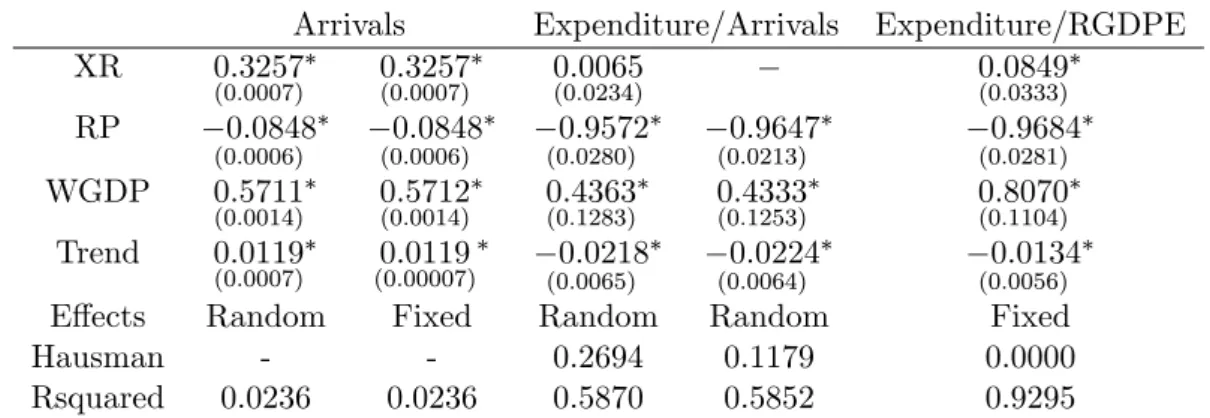
In the next subsections we analyze the results drawn from our three econometric models for tourism demand, using di¤erent proxies. Results are in Table 2 below. The last subsection will make a comparison between the three estimations for tourism demand.
[TABLE 2 ABOUT HERE]
4.1 Arrivals
The second and third columns of Table 2 show us the results for the estimations when Arrivals is the explanatory variable, using random and …xed e¤ects estimators. According to what was expected in theory, all the estimates associated to the macroeconomic variables have the correct signs and are statistically signi…cant. The determinant which has the biggest impact, in absolute value, is the World GDP per capita, followed by the nominal exchange rate. The WGDP elasticity of demand is equal to 0.57 whereas the other one equals 0.33. The impact of relative prices (-0.08) is small. The trend has a positive slope, meaning that there is a growing
trend (1.2% per year) in the number of tourists (arrivals), which is what we actually observe looking at the empirical data.
4.2 Real Expenditures per Arrivals
The fourth and …fth columns of Table 2 present results using Real Expenditures per Arrivals as a proxy for tourism demand, with the random e¤ects estimator according to usual speci…cation tests. Again, we have the expected signs, although the nominal exchange rate is not statistically signi…cant. In this case the most relevant variable is the relative prices, followed by the World GDP per capita (estimate of 0.43). In fact, the hypothesis of a relative prices (negative) unitary elasticity of real expenditure level per visitor cannot be statistically excluded from this model. Hence, the price of goods and services at the destination vis-à-vis the Rest of the World (i.e., the US) is a very important element when potential tourists make their travel decisions. O¤ course, it depends on the social economic status of the tourist, but in a global World, in which is ever more common to travel, more people of lower social economic status travel abroad, and these are the ones more sensible to price di¤erences. The estimated value associated with the trend is this time negative, which means, that we can observe a declining trend in the expenditures per tourist of about 2.2% a year. This can arise due to several factors. First, due to competition between …rms involved in the tourism industry, which is clearly growing, prices can go down. Second, since more young people are travelling and their budgets are tighter, expenditures per tourist can also decrease.
4.3 Real Expenditures per GDP
The last column of Table 2 exhibits results for the estimations when we use Real Expenditures per GDP as the explanatory variable. The speci…cation tests were computed and the …xed e¤ects estimator is the chosen one. All coe¢ cients are statistically signi…cant and have the expected signs. Con…rming the results of the previous model, the elasticity of the relative prices is essentially unitary (negative), i.e., it implies that consumers do care about price comparison when they purchase goods or services at the destination. The World GDP per capita has also a quite high elasticity (0.81). The nominal exchange rate elasticity is the smallest one in absolute value (0.08), yet positive and signi…cant, contrary to what happen in the previous model. Moreover, Real Expenditures per GDP have been decreasing at an average rate of 1.3% per year. The explanations provided in the previous subsection, apply to this one.
From the FE estimation procedure, we can obtain and rank the various individual country e¤ects. The 20 countries with the highest and the lowest values are listed in Table 3 below.
[TABLE 3 ABOUT HERE]
The maximum amount is for Macao (3.4197) while the minimum is -4.9875 (Guinea). This means that, for example, Macao’s country-speci…c characteristics are such that enable tourists to spend a ratio Expenditures/RGDPE of 30 per year (= exp(3:4)) above the average country, after controlling for all covariates in the model. Obviously, this is a signi…cant value because Macao is a small open economy that bene…ts a lot from the tourism industry.
4.4 Comparing Results
In this subsection we discuss the results of the previous three subsections. There is clearly a di¤erence on the results of the elasticities of the macroeconomic determinants when we use a proxy for tourism demand based on quantity (Arrivals) or based on value (Real Expenditures per Arrivals and Real Expenditures per GDP).
When we use Arrivals as a proxy for tourism demand the World GDP per capita is the most important determinant, with the highest elasticity in absolute value, followed by the nominal exchange rate, and the e¤ect of relative prices which, although signi…cant, is almost negligible. But in the two estimations based on expenditure proxies, the relative prices become the most important determinant of tourism demand with a negative unitary elasticity. These last two estimations emphasize the relevance of the international comparison of prices, restricted on their own budget, before people make their decision where to travel and visit. The World GDP per capita is an important determinant, either when we use Arrivals or Real Expenditures (per Arrivals or per GDP) as proxies for tourism demand, although is specially relevant when Real Expenditures per GDP is used. In these last two estimations the e¤ect of the nominal exchange rate is either non-signi…cant or small. We observe a negative trend in the expenditures estimations, pointing to a decrease in expenditure per tourist and per GDP, possibly resulting from the increase in competition, which can decrease prices. When we use Arrivals, the trend is positive, pointing to an increase in the number of people travelling. These two trends seem to represent a typical demand function, based on prices and competition.
5
Extensions
The estimates of the country-speci…c …xed e¤ects in determining the level of expenditures per GDP highlight the fact that the wealth and the size of the economy might in‡uence the tourism demand functions (c.f. Table 3 above). Thus, in this section we analyze the results of two extensions: we have partitioned the data by income level and also by Continent. These two extensions allow us to check the robustness of the macroeconomic determinants obtained before to explain the tourism demand.
5.1 Analysis by Income Level
We …rst break our data by income level using an adapted measure of the partition by income level of the World Bank. The World Bank uses the Gross National Income (GNI) per capita to breakdown countries by income level whereas in our sample we have data for nominal GDP per capita. Despite the obvious di¤erences between GNI and GDP, we rank the countries according to their GDP in our dataset and apply the intervals of the World Bank.3
Overall, there are 17.85% of low income data points (Low), 24.32% lower middle income (LowMid), 24.96% upper middle income (UpperMid) and 32.80% of high income observations (High). In order to distinguish the elasticities of the macroeconomic variables according to the in-come level, we aggregate the lower middle inin-come and upper middle inin-come groups and build two dummy variables dlit= 8 > < > : 1 if GDPit2 low income 0 if otherwise and dhit= 8 > < > : 1 if GDPit2 high income 0 if otherwise ; both of which are time-varying. Almost all countries experienced a change in income level at some point of time, the majority an upgrade in its development level.
We extend the models (1), (5), and (6) by also including the covariates interacted with dlit and dhit so that the tourism demand functions for these two groups are compared to the
reference group of middle income. More speci…cally, what was de…ned before as x0it is now
x0it + dlitx0it + dhitx0it : (7)
3
The World Bank revises the classi…cation of the world’s economies yearly, based on estimates of the current gross national income (GNI) per capita for the previous year. As of 1 July 2012, the World Bank income classi…cations by GNI per capita are as follows:
- Low income: $1,025 or less;
- Lower middle income: $1,026 to $4,035; - Upper middle income: $4,036 to $12,475; - High income: $12,476 or more.
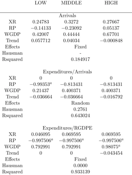
The estimation results are in Table 4. In the second column (LOW) we have b +b; then (MID-DLE) b; and in the last (HIGH) b +b: We removed the parameters that were not statistically signi…cant and that is the reason why some elasticities are the same across two or more groups.
[TABLE 4 ABOUT HERE]
The results are quite robust to the partition made to the data and the ranking of the elasticities still prevails in the partition between income levels, in all three estimations.
When Arrivals is the explanatory variable, the low and middle income countries’ results are quite similar to the original estimations, even though the coe¢ cients for relative prices and the trend are larger. The coe¢ cient for World GDP per capita is smaller. For high income countries, the sign for the relative price and the trend changes, but the coe¢ cients are small, and the coe¢ cient of the World GDP per capita is larger. The results for Arrivals as the dependent variable seem to emphasize the higher relevance of the evolution of world income to high income countries and the higher relevance of relative prices to low and middle income countries (but still smaller in absolute value than the other two elasticities). Finally, arrivals have stagnated in high income countries (drop of 0.08% a year) compensated by an enormous growth in low and middle income countries (5.7% and 4%, respectively).
When the explanatory variable is Real Expenditures per Arrivals, the results for the coef-…cients of relative prices for middle and high income countries, for the World GDP per capita for low income countries, and for the trend for low and middle income countries are those that change the most, relative to the original estimations. Results stress the importance of relative prices to low income countries in comparison to middle and high income countries and also the relevance of the World GDP per capita to middle and high income countries in comparison to low income countries. Nevertheless, the elasticity of relative prices is always the largest and only for low income group the (negative) unitary hypothesis cannot be empirically rejected. The drop of spending per tourist is more signi…cant in low and middle income countries (3.7%) than in high income countries (1.7%).
When we change the analysis to the Real Expenditure per GDP, the values for the coe¢ cients of the nominal exchange rate all decrease slightly for all income levels, in terms of the relative prices the opposite happens, and for the World GDP per capita the results change for high income countries only. Again, elasticity of RP is the largest, with all groups having unitary elasticity, but now the elasticity of WGDP is closer to one. In fact, for the high income group,
unitary elasticities exist for RP and WGDP, meaning that both e¤ects are equally important and very elastic. The Real Expenditure per GDP stabilized for low and middle income countries but dropped 4.3% per year in high income countries.
5.2 Analysis by Continent
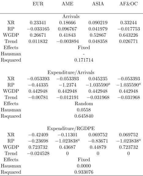
Additionally, we also separate our data by Continent. There are 21.55% of countries in Asia, 21.10% in Europe, 24.31% in Africa, 9.17% in Oceania and 23.85% in America. We aggregate Africa and Oceania. Thus, and similarly to the income level partition, we now extend the original list of covariates to include the interactions with dummies for Europe, America and Asia so that the tourism demand models for these three groups are compared to the reference group of Africa and Oceania. Obviously, all dummies are time-invariant. The results are in Table 5, distinguishing the estimated elasticities in Europe (EUR), America (AME), Asia (ASIA) and Africa and Oceania (AF&OC), after eliminating the parameters that were not statistically signi…cant in the models.
[TABLE 5 ABOUT HERE]
As we can see, the results are not quite as robust as in the previous section, although the ranking of the elasticities only change in the case of Real Expenditures per GDP, for Europe, where the ordering changes substantially. More importantly, the nominal exchange rate happens to be statistically signi…cant now for the second model and in several situations the sign of the elasticity is not the expected one.
In the speci…cation for Arrivals, the sign of the estimated coe¢ cient of RP for America and Asia is not according to theory (is positive instead of negative) and contradicts all previous estimations. The relative positions of the coe¢ cients (elasticities) for the World GDP per capita and the nominal exchange rate are quite robust across groups. Only for Europe, the elasticity of XR gets close enough from the one of WGDP, the largest. It is in Africa and Oceania that the elasticities of XR and WGDP are the largest compared to any other group. This means that, for Arrivals, AF&OC are the most sensitive continents to the macroeconomic drivers. For the period under analysis, the number of arrivals slightly dropped in America (0.4% a year) but rose elsewhere (from 1.2% in Europe to 4.8% in Asia).
When Real Expenditures per Arrivals is the explanatory variable, relative prices and the World GDP per capita maintain their relative position for all continents, although relative
prices have a much lower impact in Europe than in the other continents. It is in fact the only continent for which the elasticity of RP is smaller than one, in absolute value. The elasticity of WGDP is the same across groups (0.44). The exchange rate only has the correct sign in Asia. The Real Expenditures per Arrivals have fallen over the years (from 0.8% in Europe to 3.2% in Asia, Africa and Oceania).
For the estimations in which we use Real Expenditures per GDP as the dependent variable, relative prices have again a much lower impact in Europe, and a slightly lower impact in Asia, compared to the remaining continents (these with unitary elasticity). The World GDP per capita has a much lower impact in America and Asia, relatively to the other continents. By contrasting the two elasticities, only in Europe the coe¢ cient of WGDP is larger than RP. That is, only in Europe the tourist’s expenditures is less sensitive to changes in prices than in wealth. All continents have experienced a constant level of Real Expenditures per GDP except in Europe where it dropped 2.5% per year. The wrong expected sign for the nominal exchange rate in Europe and America, in the last two regressions, can be explained by business travelling to these two continents that is not in‡uenced by the depreciation of the nominal exchange rate.
6
Conclusion
This work analyzes the in‡uence of some key macroeconomic determinants, such as, the nominal exchange rate, relative prices, and the World GDP per capita, on the World tourism demand, namely on the inbound number of visitors and tourism expenditures, for a panel of 218 countries observed between 1995 and 2012.
We have estimated three models, using three di¤erent proxies for tourism demand - Arrivals, as a measure of tourism quantity, and Real Expenditures per Arrivals, and Real Expenditures per GDP, measuring tourism value. There is evidence that an increase in the World’s GDP per capita, a depreciation of the national currency, and a decline of relative domestic prices do help boosting the number of arrivals and the correspondent expenditure level. The World GDP per capita is more relevant when we use arrivals as our dependent variable, but relative prices become the most important when we use expenditures as the proxy for tourism demand. In particular, we cannot reject the hypothesis of a relative prices (negative) unitary elasticity of real expenditures, i.e., consumers do care about price comparison when they choose destination and purchase goods or services at the destination.
On average, the number of tourists (arrivals) grew 1.2% per year whereas relative expen-ditures declined about 2% per year. In a global World, it becomes more common to travel abroad, including more people of lower social economic status, and …erce competition between …rms involved in the tourism industry may be pushing prices down.
Additionally, we have also partitioned our data by income level and by continent. Results are robust in the …rst partition, but less robust in the second, although the main conclusions still hold. The results seem to emphasize the relevance of the world income to high income countries and of the relative prices to low and middle income countries, in determining tourism demand. For the period under analysis, arrivals have stagnated in high income countries and the drop in the expenditure levels per tourist is more signi…cant in low and middle income economies.
The relative prices have a much lower impact in Europe, when compared to other continents. Arrivals in Europe do change with nominal exchange rates almost as with the World GDP and in Africa and Oceania both elasticities are the largest compared to any other group. That is, Africa and Oceania are the most in‡uenced by the macroeconomic drivers. The expenditure level per tourist elasticity of the World GDP is the same for all continents. Also, the World GDP per capita has a much lower impact in America and Asia, relatively to the other continents, in determining the expenditures per GDP. Finally, Asia experienced the highest increase in arrivals (4.8% a year) but it was also the continent (ex-aequo with Africa and Oceania) whose expenditures per arrivals have fallen the most (3.2% per year).
The panel we use in this paper is very complete at the micro level since it covers essentially all countries in the world. Nevertheless, the time series information is somehow limited because the number of years it covers is not that signi…cant and some variables of the models are not observed for some countries over the entire period. In the future, it shall be important to study the macroeconomic determinants in tourism demand once more time observations become available to practitioners.
References
[1] Baltagi, B. H. 2013. Econometric Analysis of Panel Data, 5th edition, John Wiley, New York.
[2] Cameron, A. C. & Trivedi, P. K. 2005. Microeconometrics: Methods and Applications, Cambridge University Press, New York.
[3] Chang, C.-L. & Mcaleer, M. 2012. Aggregation, heterogeneous autoregression and volatility of daily international tourist arrivals and exchange rates. Japanese Economic Review, 63 (3): 397-419.
[4] Chao, C.-C., Lu, L.-J., Lai, C.-C., Hu, S.-W. & Wang, V. 2013. Devaluation, pass-through and foreign reserves dynamics in a tourism economy. Economic Modelling, 30 (1): 456-461. [5] Chen, M.-H., Lin, C.-P. & Chen, B. T. 2015. Drivers of Taiwan’s Tourism Market Cycle.
Journal of Travel & Tourism Marketing, 32 (3): 260-275.
[6] Cheng, K. M., Kim, H. & Thompson, H. 2013a. The real exchange rate and the balance of trade in US tourism. International Review of Economics and Finance, 25: 122-128.
[7] Cheng, K. M., Kim, H. & Thompson, H. 2013b. The exchange rate and US tourism trade, 1973-2007. Tourism Economics, 19 (4): 883-896.
[8] De Vita, G. 2014. The long-run impact of exchange rate regimes on international tourism ‡ows. Tourism Management, 45: 226-233.
[9] De Vita, G. & Kyaw, K. S. 2013. Role of the exchange rate in tourism demand. Annals of Tourism Research, 43: 624-627.
[10] Dritsakis, N. 2012. Tourism development and economic growth in seven Mediterranean countries: A panel data approach. Tourism Economics, 18 (4): 801-816.
[11] Dwyer, L. & Forsyth, P. 2002. Destination price competitiveness: Exchange rate changes versus domestic in‡ation. Journal of Travel Research, 40 (3): 328-336.
[12] Ghartey, E. E. 2013. E¤ects of tourism, economic growth, real exchange rate, structural changes and hurricanes in Jamaica. Tourism Economics, 19 (4): 919-942.
[13] Harvey, H., Furuoka, F. & Munir, Q. 2013. The role of tourism and exchange rate on economic growth: Evidence from the BIMPEAGA. Economics Bulletin, 33 (4): 2756-2762. [14] Hausman, J. 1978. Speci…cation Tests in Econometrics. Econometrica, 46 (6): 1251-1271. [15] International Monetary Fund, World Economic Outlook Database [accessed in December,
[16] Kiliç, C. & Bayar, Y. 2014. E¤ects of Real Exchange Rate Volatility on Tourism Receipts and Expenditures in Turkey. Advances in Management & Applied Economics, 4 (1): 89-101. [17] Lee, C.-K., Var, T. & Blaine, T.W. 1996. Determinants of Inbound Tourist Expenditures.
Annals of Tourism Research, 23 (3): 527-542.
[18] Odhiambo, N. M. 2011. Tourism development and economic growth in Tanzania: Empirical evidence from the ARDL-bounds testing approach. Dissertation, University of South Africa. [19] Penn World Table, version 7.1 [accessed in April, 2014]
https://pwt.sas.upenn.edu/php_site/pwt_index.php.
[20] Penn World Table, version 8.0 [accessed in April, 2014] http://www.rug.nl/research/ggdc/data/penn-World-table.
[21] Saayman, A. & Saayman, M. 2013. Exchange rate volatility and tourism - Revisiting the nature of the relationship. European Journal of Tourism Research, 6 (2): 104-121.
[22] Salman, A. K., Shukurb, G. & von Bergmann-Winberg, M.-L. 2007. Comparison of Econo-metric Modelling of Demand for Domestic and International Tourism: Swedish Data. Cur-rent Issues in Tourism, 10 (4): 323-342.
[23] Schi¤, A. & Becken, S. 2011. Demand elasticity estimates for New Zealand tourism. Tourism Management, 32 (3): 564-575.
[24] Sequeira T. N. & Campos C. 2007. International Tourism and Economic Growth: A Panel Data Approach. Advances in Modern Tourism Research, 153-163.
[25] Sequeira T. N. & Nunes P. M. 2008a. Does tourism in‡uence economic growth? A dynamic panel data approach. Applied Economics, 40 (18): 2431-2441.
[26] Sequeira T. N. & Nunes P. M. 2008b. Does country risk in‡uence international tourism? A dynamic panel data analysis. Economic Record, 84: 223-236.
[27] Wooldridge, J. M. 2010. Econometric Analysis of Cross Section and Panel Data, 2nd edition, MIT Press, Cambridge, MA.
[29] World Tourism Organization, World Tourism Data [accessed in April, 2014] http://data.un.org/DocumentData.aspx?q=Tourism&id=369
Table 1: Variables
POP Population –in millions
XR Exchange Rate, National Currency/U.S. Dollars
RGDPE Expenditure-side real GDP at chained PPPs –U.S. dollars in millions, 2005=100
CPI Consumer Price Index (2005=100)
Expenditure Tourism real expenditure in the country–U.S. dollars in millions, 2005=100 Arrivals (TF) or (VF) Arrivals of non-resident tourists (visitors) at national borders- in thousands WGDP World Gross Domestic Product, Current prices–U.S. dollars in billions
Table 2: Results for the Three Speci…cations
Arrivals Expenditure/Arrivals Expenditure/RGDPE
XR 0:3257 (0:0007) 0:3257(0:0007) 0:0065(0:0234) 0:0849(0:0333) RP 0:0848 (0:0006) 0:0848 (0:0006) 0:9572 (0:0280) 0:9647 (0:0213) 0:9684 (0:0281) WGDP 0:5711 (0:0014) 0:5712(0:0014) 0:4363(0:1283) 0:4333(0:1253) 0:8070(0:1104) Trend 0:0119 (0:0007) (0:00007)0:0119 (0:0065)0:0218 0:0224 (0:0064) 0:0134 (0:0056)
E¤ects Random Fixed Random Random Fixed
Hausman - - 0.2694 0.1179 0.0000
Rsquared 0.0236 0.0236 0.5870 0.5852 0.9295
Note: stands for statistically signi…cant; All log-log speci…cations; Intercept not included in the table; Hausman test p-value
Table 3: Estimated Country Speci…c E¤ects Expenditures per RGDPE Model
Highest Smallest
MACAO, CHINA 3:4197 GUINEA 4:9875
MALDIVES 3:1873 BANGLADESH 3:8436
BAHAMAS 3:0571 BURUNDI 3:6901
CYPRUS 2:4474 TAJIKISTAN 2:7431
BARBADOS 2:4446 NIGERIA 2:3139
FIJI 2:3228 CENTRAL AFRICAN REPUBLIC 2:1740
MALTA 2:2996 BELARUS 2:0851
LUXEMBOURG 2:2955 PAKISTAN 2:0642
JAMAICA 2:0122 JAPAN 2:0336
BELIZE 2:0044 INDIA 1:9715
Table 4: Results for the Partition by Income Level
LOW MIDDLE HIGH
Arrivals XR 0:24783 0:3272 0:27667 RP 0:14133 0:23092 0:05137 WGDP 0:42007 0:44444 0:67701 Trend 0:057712 0:04034 0:000848 E¤ects Fixed Hausman -Rsquared 0.184917 Expenditures/Arrivals XR 0 0 0 RP 0:99353a 0:813431 0:813431 WGDP 0:21437 0:400371 0:400371 Trend 0:036664 0:036664 0:016792 E¤ects Random Hausman 0.2761 Rsquared 0.643024 Expenditures/RGDPE XR 0:046095 0:069595 0:069595 RP 0:997506a 0:997506a 0:997506a WGDP 0:792991 0:792991 0:98075a Trend 0 0 0:043454 E¤ects Fixed Hausman 0.0000 Rsquared 0.933139
Note: all coe¢ cients are statistically signi…cant at 5% level; All log-log speci…cations; Hausman test p-value
Table 5: Results for the Partition by Continent
EUR AME ASIA AF&OC
Arrivals XR 0:23341 0:18666 0:090219 0:33244 RP 0:033165 0:096767 0:041979 0:017753 WGDP 0:26671 0:41843 0:52867 0:643226 Trend 0:011832 0:003894 0:048358 0:026771 E¤ects Fixed Hausman -Rsquared 0.171714 Expenditure/Arrivals XR 0:053393 0:053393 0:045235 0:053393 RP 0:44335 1:2374 1:035590a 1:035590a WGDP 0:442948 0:442948 0:442948 0:442948 Trend 0:00781 0:012191 0:031968 0:031968 E¤ects Random Hausman 0.0558 Rsquared 0.645840 Expenditure/RGDPE XR 0:42409 0:11301 0:069752 0:069752 RP 0:23698 1:023838a 0:83671 1:023838a WGDP 0:723732 0:43687 0:44879 0:723732 Trend 0:024528 0 0 0 E¤ects Fixed Hausman 0.0000 Rsquared 0.933076
Note: all coe¢ cients are statistically signi…cant at 5% level; All log-log speci…cations; Hausman test p-value