micro-climate and macro-biogeographic
patterns of intertidal rocky shore organisms
Rui Seabra Alves Martinho
Supervisors:
David S. Wethey
António M. Santos
Fernando P. Lima
grau de Doutor em Biodiversidade, Genética e Evolução. Porto, 2015.
Em todas as publicações decorrentes deste trabalho é devidamente referido que as instituições de origem do doutorando Rui Seabra Alves Martinho são:
• Departamento de Biologia, Faculdade de Ciências da Universidade do Porto, R. Campo Alegre, s/n, 4169-007 Porto, Portugal.
• CIBIO-InBIO, Centro de Investigação em Biodiversidade e Recursos Genéticos, Campus Agrário de Vairão, Universidade do Porto, 4485-661, Vairão, Portugal.
Este trabalho foi apoiado financeiramente pela Fundação para a Ciência e a Tecnologia (FCT) através de uma bolsa de doutoramento (ref. SFRH/BD/68521/2010) e dois projectos científicos (HINT, ref. PTDC/MAR/099391/2008, e COASTAL4CAST, ref. PTDC/MAR/117568/2010), e pelo FEDER (FCOMP-01-0124-FEDER-010564, FCOMP-01-0124-FEDER-020817).
Na elaboração desta tese, e nos termos do número 2 do Artigo 4◦ do Regulamento Geral dos Terceiros Ciclos de Estudos da Universidade do Porto e do Artigo 31◦ do D.L. 74/2006, de 24 de Março, com a nova redação introduzida pelo D.L. 230/2009, de 14 de Setembro, foi efetuado o aproveitamento total de um conjunto coerente de trabalhos de investigação já publicados ou submetidos para publicação em revistas internacionais indexadas e com arbitragem científica, os quais integram alguns dos capítulos da presente tese. Tendo em conta que os referidos trabalhos foram realizados com a colaboração de outros autores, o candidato esclarece que, em todos eles, participou ativamente na sua concepção, na obtenção, análise e discussão de resultados, bem como na elaboração da sua forma publicada.
"Once I get on a puzzle, I can’t get off" - Richard Feynman
"Somewhere, something incredible is waiting to be known" - Carl Sagan
"Hofstadter’s Law: It always takes longer than you expect, even when you take into account Hofstadter’s Law"
This work was mainly supported by Fundação para a Ciência e a Tecnologia (FCT), under contract number SFRH/BD/68521/2010. I was also beneficiary of financial and logistic support from the Centro de Investigação em Biodiversidade e Recursos Genéticos (CIBIO-InBIO), and from the Departamento de Biologia da Faculdade de Ciências da Universidade do Porto (DB-FCUP). In addition, two research project grants from FCT/FEDER (HINT, ref. PTDC/MAR/099391/2008, FCOMP-01-0124-FEDER-010564, and COASTAL4CAST, ref. PTDC/MAR/117568/2010, FCOMP-01-0124-FEDER-020817) covered most costs related to field work and the set-up of the aquaria facilities.
I feel very fortunate for all the good friends and colleagues who collectively carried me during this demanding period of my life. A special thank goes to my surf buddies Pedro Costa, Pedro Monterroso and Pedro Pinho, and my high-school mates Susana Pedro, Julio Cabral and Miguel Polónia, with whom I shared some of the most memorable moments of my life, filling me with energy for the tasks ahead.
Arriving at CIBIO was truly a random walk process, and numerous people were determinant in saving me from going astray. As an undergraduate, my friends Ana Goios, André Maia, Daniela Ferreira, Fabian Sá and Pedro Moreira made biology classes much easier and entertain-ing. In particular, André Maia provided me with all the lecture notes I was too lazy to take, but then badly needed (recurrently). Paula Tamagnini, my supervisor during an undergraduate project and the MSc thesis, was instrumental in getting me to publish, and wisely steered me away from lab work and into the field, where she knew I belonged even before I realized it. During my stay in CIIMAR, Vitor Vasconcelos was incredibly welcoming, and still is a great source of inspiration. Lastly, during a seemingly unimportant dinner, Diana Castro and Pedro Monterroso revealed the existence of a research centre named CIBIO, which until then I had been oblivious about.
After eventually arriving at CIBIO, the work leading to this thesis was filled with hurdles that I was only able to overcome with the help of many. Much of this work would not have been possible without free access to numerous software tools, databases and instructions (R Project,
Arduino, Google Maps, StackExchange, among many others). The level of spontaneous
collaboration that arises within these communities of contributors (agencies and individuals) never ceases to amaze me, and is a source of inspiration. For their invaluable help during lab/field work, great discussions and friendship, I thank my research colleagues Cristián Monaco,
Filipa Gomes, Lara Sousa, Nick Burnett, Pedro Ribeiro, Raquel Xavier and Stephen Sabatino, and my "co-co-supervisors" Jerry Hilbish and Sarah Woodin. I also extend my gratitude to the unparalleled Nuno Queiroz, for the constructive scientific discussions, hilariously awkward moments, multiplayer tank games and fantastic friendship. Notwithstanding the relevance all the other support I received, the guidance, friendship and incentive provided by my dream team of supervisors was the single most important factor leading to the completion of this thesis. Thus, I would like to thank David Wethey for all the amazing insights on environmental analysis, biogeography, programming and electronics, as well as for hosting me in his peculiar lab in the University of South Carolina, Columbia. I would also like to thank António Múrias, the go-to person for issues on biodiversity, statistics and programming (countless issues...), and a great joke teller. Finally, I would like to express my deepest gratitude to Fernando Lima. Fernando is, hands down, the best supervisor I could have ever had, instilling in me the right amount of drive, curiosity and responsibility necessary to get things done, all while mastering the balance between never lowering the bar on research quality and fostering a great friendship. I am extremely happy to have shared epic field work trips, countless stories and bad jokes, and nervous multiplayer tank games with such a friend (I hope to one day supervise like you...).
Lastly, my family, which makes up a large part of me. I thank all my cousins, aunts and uncles for the memories and support. To Ana Paula and José Queiroga, I thank the love and support, expressed during so many weekend dinners spent together. I thank my grandparents, which have always inspired me to work harder - especially my grandmother Glória Neves. A special thank is also due to my uncle Zeferino Martinho "Fino", one of the wittiest and good spirited persons I have ever known, showing constant interest for my advancements in this project. In equal amounts, I thank my unconditionally loving and supportive parents, who have always been there for me, who have taught me to put problems into perspective ("o que é isso comparado com o raio da Terra?"), and who, from the very beginning, have fueled my passion for science and nature.
... and Catarina, my wife, my life companion, my friend, my lover. Together we faced turbulent seas, but you were always loving and caring. These past years have been incredible, and sharing field work with you was absolutely amazing. For all the travel and good memories that were, and for all that will be... I would have been lost without you.
Temperature is considered one of the most important drivers of biological processes affecting the physiology and ecology of both endotherms and ectotherms. Intertidal species, despite their marine ancestry, are periodically exposed to extremely stressful and variable terrestrial conditions, and thus have long been regarded as ideal models for understanding how the physical environment drives physiology, biotic interactions, and ecological patterns in nature. The rocky intertidal environment is remarkably variable at a centimeter scale, and the complexity of its small-scale topography ensures that most locations encapsulate a myriad of contrasting microhabitats for species to explore, with vastly different thermal characteristics. Yet, the importance of this variability in determining large-scale macro-ecological processes remains virtually unknown. This thesis takes advantage of this singular system to gain insights on the basic ecological process driving the distribution of species, setting their range limits, and dictating change.
The first chapter sets the context of this thesis by introducing the main theoretical concepts, environmental setting and studied species, and briefly identifying the current gaps in knowledge. The general introduction ends with an outline of the rationale and with a list of the manuscripts that compose the thesis.
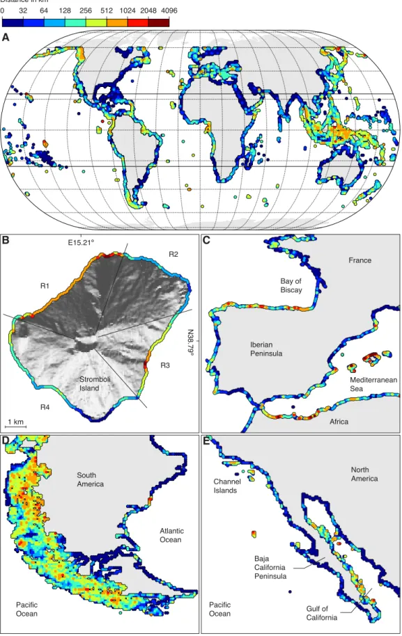
The second chapter aims at unravelling the intricate patterns of environmental variability. Firstly, the complexity of the thermal environment of rocky shores along the European Atlantic coast is detailed, showing that thermal differences between sun-exposed and shaded microhabi-tats are higher than those related to seasons, latitude or shore level. Secondly, a global look into the role of shading provided by coastal topography reveals that in some regions topographical shading may be a major source of habitat complexity. Although likely, the biological significance of this new pattern is yet to be ascertained, opening exciting new opportunities for future research.
Focusing on the microhabitat level, the third chapter sets out to evaluate the implications of the striking levels of environmental variability identified. Through the quantification of the heat-shock proteins present in individuals of Patella vulgata Linnaeus, 1758 from different microsites along the European Atlantic coast, it is shown that different thermal histories are consistently associated with differences in physiological performance. The link found confirms that the limiting effects of temperature, rather than being related to latitude, seem to be tightly associated with microsite variability, which therefore is likely to have profound effects on the way local populations (and species) respond to climatic changes. In order to evaluate the relative contribution of water and air temperature during emersion for the build-up of thermal stress, a modern and simplified infrared heartbeat rate sensing system was designed.
This technique overcomes obstacles encountered with previous methods of heartbeat rate measurement, and due to the sensor’s small size, versatility, and noninvasive nature, creates new possibilities for studies across a wide range of organismal types. Making use of this new apparatus, a set of laboratorial experiments shows that thermal stress is directly linked to elevated water temperature, while warm air temperature during emersion plays a secondary role. In conjunction with population density data, these results suggest that high water temperature represents a threshold that the intertidal limpet P. vulgata is unable to tolerate.
The fourth chapter builds on the previous findings, exploring how complex biogeographic responses to climatic changes may arise from the thermal complexity of the intertidal environ-ment. Importantly, it emphasizes that unless the appropriate temperature metrics (e.g., daily range, min, max) are analyzed, the impacts of climate change may be misinterpreted.
A temperatura desempenha um papel crucial no controlo de inúmeros processos biológicos, afetando a fisiologia e ecologia de animais endotérmicos e ectotérmicos. No que se refere aos animais ectotérmicos que ocorrem em zonas intertidais, a sua ascendência marinha significa que a exposição periódica a condições terrestres resulta em elevados níveis de stress, podendo por isso ser considerados modelos ideais para o estudo do modo como o ambiente físico controla a fisiologia, interacções bióticas e padrões ecológicos na natureza. As condições ambientais na zona entre marés de praias rochosas são extremamente variáveis, e a complexidade da sua micro-topografia significa que a maioria dos locais encapsula uma grande quantidade de micro-habitats que as espécies que aí habitam podem potencialmente explorar. Contudo, a importância desta variabilidade para o desenrolar de processos macro-ecológicos ainda permanece praticamente desconhecida. Fazendo uso deste sistema singular, esta tese tem por objetivo a investigação dos processos ecológicos básicos que determinam a distribuição das espécies e que modelam a resposta destas a alterações ambientais.
O primeiro capítulo define o contexto desta tese, introduzindo os principais conceitos teóricos, descrevendo as características mais relevantes do ambiente e das espécies estudadas, identificando também as principais lacunas no conhecimento atual. A introdução geral termina com uma breve descrição do encadeamento das várias tarefas desenvolvidas, bem como com uma lista dos artigos científicos que compõem a tese.
O segundo capítulo tem como objetivo a caracterização da variabilidade ambiental. No primeiro trabalho é feita uma descrição da complexidade do ambiente térmico em praias rochosas ao longo da costa Atlântica da Europa. Os resultados mostram que as diferenças térmicas entre micro-habitats sombreados e expostos ao sol excedem as diferenças associadas às estações do ano, latitude ou posição na zona intertidal. No segundo trabalho é apresentada uma perspetiva global do papel desempenhado pela topografia costeira como fonte de complexidade ambiental. Ainda que provável, a relevância deste novo padrão ambiental permanece especulativa, o que por seu turno abre novas e interessantes vias de trabalho futuro.
Centrando a atenção na escala do micro-habitat, o terceiro capítulo tem como objetivo avaliar as implicações dos elevados níveis de variabilidade ambiental identificados. Através da quantificação dos níveis de proteínas de choque térmico (heat-shock proteins) presentes em indivíduos de Patella vulgata Linnaeus, 1758 recolhidos de micro-habitats diferentes ao longo da costa Atlântica Europeia, demonstrou-se a associação entre o historial térmico e diferenças no desempenho fisiológico destes animais. A identificação desta conexão confirma que o efeito limitador da temperatura está fortemente associado à variabilidade entre micro-habitats - e não à latitude, o que por sua vez tem diversas implicações na forma como
populações locais (ou mesmo espécies) respondem a alterações ambientais. Seguidamente, de forma a avaliar o contributo relativo da temperatura da água e do ar para os níveis de stress térmico, foi desenvolvido um sistema moderno e simplificado de medição de atividade cardíaca usando radiação infravermelha. A utilização desta técnica permite ultrapassar vários obstáculos frequentemente encontrados noutras técnicas de medição de atividade cardíaca. O tamanho reduzido do sensor, aliado à versatilidade e carácter não invasivo do sistema, permite a realização de inúmeros tipos de estudos em invertebrados com diversas formas corporais. Utilizando este novo equipamento, foram realizadas experiências laboratoriais que demonstraram que o stress térmico está directamente relacionado com temperaturas de água elevadas, tendo a temperatura do ar um papel secundário. Estes resultados, em conjunto com dados de densidade populacional, sugerem que valores elevados de temperatura de água representam um limite que a lapa P. vulgata não é capaz de tolerar.
O quarto capítulo recupera os resultados anteriores e explora a forma como alterações climáticas podem levar a respostas biogeográficas não-intuitivas devido à complexidade do ambiente térmico das zonas intertidais, salientando a importância da utilização das métricas da temperatura (e.g., amplitude diária, mínimo, máximo) mais ajustadas à questão e ao organismo em estudo.
Por último, as conclusões extraídas em todos os trabalhos que compõem esta tese são discutidos e sintetizados numa discussão geral.
1 General Introduction 1
1.1 Temperature, a major driver of species’ distribution patterns . . . 1
1.2 The rocky intertidal . . . 1
1.2.1 Environmental mosaic . . . 2
1.2.2 The European Atlantic coast . . . 2
1.3 Climate change. . . 2
1.4 Complex biological responses . . . 3
1.5 General objectives . . . 3
1.6 Submitted and published manuscripts . . . 3
2 The environment at multiple scales 5 2.1 Side matters: Microhabitat influence on intertidal heat stress over a large geographical scale . . . 5
2.1.1 Abstract . . . 5
2.1.2 Introduction . . . 5
2.1.3 Material and Methods . . . 6
2.1.4 Results . . . 10
2.1.5 Discussion . . . 12
2.1.6 Acknowledgements . . . 16
2.1.7 Supplementary data . . . 17
2.2 Topographical shading shapes coastal habitat complexity . . . 21
2.2.1 Abstract . . . 21
2.2.2 Main text . . . 21
2.2.3 Acknowledgements . . . 26
3 Patterns of thermal stress 27 3.1 Loss of thermal refugia near equatorial range limits . . . 27
3.1.1 Abstract . . . 27
3.1.2 Introduction . . . 27
3.1.3 Material and methods . . . 29
3.1.4 Results . . . 32
3.1.5 Discussion . . . 34
3.1.6 Acknowledgements . . . 39
3.2 An improved noninvasive method for measuring heartbeat of intertidal animals 41 vii
3.2.1 Abstract . . . 41
3.2.2 Introduction . . . 41
3.2.3 Material and Methods . . . 42
3.2.4 Assessment. . . 44
3.2.5 Discussion . . . 47
3.2.6 Acknowledgements . . . 51
3.3 Equatorial range limits of an intertidal ectotherm are more linked to water than air temperature. . . 53 3.3.1 Abstract . . . 53 3.3.2 Introduction . . . 53 3.3.3 Methods . . . 54 3.3.4 Results . . . 59 3.3.5 Discussion . . . 62 3.3.6 Acknowledgements . . . 65 3.3.7 Appendix A . . . 65 4 Biogeographic patterns 67 4.1 Understanding complex biogeographic responses to climate change . . . 67
4.1.1 Abstract . . . 67
4.1.2 Main text . . . 67
4.1.3 Material and Methods . . . 68
4.1.4 Results and Discussion . . . 70
4.1.5 Acknowledgements . . . 73
5 General discussion 75
3.1 Geographical locations and respective sampling dates. . . 30
3.2 Two-factor ANOVA to measure the effect of exposure to solar radiation and sampling location on the endogenous levels of Hsp on Patella vulgata . . . 33
3.3 Bill of Materials for the IR cardiac sensing amplification circuit . . . 44
2.1 Robolimpet deployment locations along the Atlantic coast of the Iberian Peninsula 7
2.2 Example of a Taylor diagram . . . 9
2.3 Body temperature profiles obtained by robolimpets deployed at different microhabitats 11
2.4 30-day rolling average of standard variation of temperature profiles, and 30-day rolling average of daily temperature maxima for São Lourenço, in W Iberia . . . . 12
2.5 Taylor diagrams for robolimpet temperatures at Biarritz during a two-hour interval around high tide . . . 13
2.6 Taylor diagrams for robolimpet temperatures at Biarritz during a two-hour interval around low tide . . . 14
2.7 Taylor diagrams for robolimpet temperatures at Biarritz during the entire tide. . . 15
2.8 Data coverage map showing the number of operational robolimpets at a given time 17
2.9 30-day rolling average of standard variation of temperature profiles within the 13 sampled locations . . . 18
2.10 30-day rolling average of daily temperature maxima of temperature profiles within the 13 sampled locations . . . 19
2.11 Taylor diagrams for robolimpet temperatures measured within the 13 sampled locations, during a two-hour interval around high tide, a two-hour interval around low tide and the entire tide, at three intertidal levels (low-, mid- and high-intertidal) 20
2.12 Topographical shading along the world’s coastlines . . . 23
2.13 Latitudinal breakdown of the TPI in 1-degree latitude bins and the curve of yearly average potential radiation . . . 24
3.1 Hsp70 levels and abundances of Patella vulgata along the European Atlantic coast 29
3.2 Correlation between Hsp70 and temperatures experienced prior to sample collection 35
3.3 Temperature as a potential limiting factor for Patella vulgata . . . 36
3.4 Flowchart of the heartbeat signal from the IR sensor to the data logging device . . 42
3.5 Functional schematic diagram of IR cardiac sensing amplification circuit . . . 43
3.6 Unfiltered heartbeat signals of the limpet Cellana grata, the mussel Septifer virgatus, and the mud crab Panopeus herbstii . . . 45
3.7 Heartbeat patterns of an Atlantic blue crab (Callinectes sapidus) measured simul-taneously with the standard impedance method and with IR sensors . . . 46
3.8 Variation in measurements of the heartbeat signal of the mussel Septifer virgatus with the IR sensor placed on three regions on the shell . . . 47
3.9 Cardiac frequency of a china limpet (Patella vulgata) exposed to 7 d of simulated tides under laboratory conditions . . . 48
3.10 Examples of heartbeat signals of P. vulgata recorded under various laboratory
conditions . . . 49
3.11 Map of the study area and average daily temperature profiles effectively experienced by limpets in each of the four stressful treatments . . . 55
3.12 Cardiac activity of P. vulgata . . . 60
3.13 Relationship between abundance of P. vulgata and temperature recorded by robolimpets . . . 61
3.14 Pattern of co-occurrence of water and air temperatures at all studied shores, based on temperatures recorded by the robolimpets . . . 62
3.15 Long-term analysis of the occurrence of extreme water temperature for the period 1951-2099 along coastal areas from south Portugal to northwest France . . . 63
4.1 Patterns of temperature metrics across the European Atlantic intertidal ecosystem 69 4.2 Climate change can generate complex biogeographic responses. . . 72
5.1 Four years of robolimpet data from mid-intertidal microhabitats . . . 76
5.2 Aquaria facility and methodologies for physiological experiments . . . 78
The final goal of biogeography is to understand why organisms exist where they do today, and where will they exist in the future, especially in face of change. Thus, unsurprisingly, distribution patterns, and the factors that control them, comprise a vast portion of the research effort of biogeographers. However, despite considerable attention and effort, numerous gaps persist in our comprehension of species’ distributions. In particular, understanding how environmental factors acting at the scale of organisms are translated into distribution patterns remains a remarkably complex task. Still, those difficulties have not deterred researchers from addressing the issue, especially as society grows conscious of the impending biological impacts brought about by climate change. In this thesis, I analyze environmental complexity and attempt to shed light on the mechanisms by which the influence of microclimate on organisms is scaled up, eventually determining species’ distributions. Results are interpreted not only in the context of climatic changes, but also in terms of their contribution to fundamental ecology. Due to their remarkable environmental complexity, and building on centuries of research, attention was focused on the thermal regimes of intertidal rocky shores of the European Atlantic coast.
1.1
Temperature, a major driver of species’ distribution
patterns
Temperature controls the pace of biochemical reactions, and beyond certain levels it can damage an organism’s biochemical machinery. The pervasive influence of temperature has long been recognized, and it is considered to be one of the most important drivers of biological processes on rocky shore ecosystems, affecting the physiology (Dahlhoff et al., 2001; Somero,
2002; Fuller et al., 2010; Hofmann and Todgham, 2010) and ecology (Porter and Gates, 1969;
Wethey, 2002; Helmuth et al.,2006a; Yamane and Gilman, 2009) of intertidal species. Owing to its spatial heterogeneity, temperature is also a key factor in determining the distribution patterns and range limits of species (Southward,1958; Southward et al., 1995;Helmuth,1998;
Sagarin et al., 1999; Helmuth et al., 2006a; Lima et al., 2007a; Wethey and Woodin, 2008;
Berke et al., 2010).
1.2
The rocky intertidal
The rocky intertidal zone, which lies between the high and low tide marks on the shores of the world’s oceans, has long served as a natural laboratory for examining relationships between abiotic stresses, biotic interactions, and ecological patterns in nature (Orton, 1929;
Southward, 1958; Connell, 1972; Wethey, 1984; Bertness et al., 1999; Somero, 2002). The intertidal environment is remarkably dynamic, and despite their marine ancestry, organisms inhabiting there are periodically exposed to extremely stressful and variable terrestrial conditions (Southward, 1958; Southward et al., 1995; Raffaelli and Hawkins,1996; Denny and Wethey,
2000; Harley, 2008).
1.2.1
Environmental mosaic
The thermal regimes of intertidal ecosystems are inherently complex. During high tide they are dominated by the stability of water temperature, while during low tide air temperature, humidity, solar radiation and wind generate highly variable temperature profiles. More importantly, given that most intertidal organisms are small in size, the micro-topographical complexity of rocky outcrops ensures that most shores encapsulate a myriad of microhabitats for species to explore, with vastly different thermal profiles (Helmuth, 1998, 2002; Wethey, 2002; Helmuth et al.,
2005; Harley,2008;Lima and Wethey,2009). In fact, the availability of such microhabitats has been recognized as a major factor determining the distribution of intertidal species, particularly towards the limits of their distribution ranges (Helmuth et al., 2006a; Bennie et al.,2008). In addition, micro-scale variability of desiccation and wave impact forces (Foster,1971;Denny et al.,
1985;McMahon, 1990; Burrows et al., 2008) further enhances intertidal habitat complexity.
1.2.2
The European Atlantic coast
There are various reasons why the European Atlantic coast is the ideal location for the study of the interplay between environmental factors and species’ distributions. First and foremost, this region of the world has long been the subject of a vast research effort in numerous fields, resulting in a continuous record of the environment and organisms inhabiting its intertidal ecosystem which dates back many decades (Orton, 1929; Fischer-Piette, 1935;
Smith,1935; Evans,1948; Southward and Crisp, 1952; Fischer-Piette, 1953; Southward and Crisp, 1954). This provides researchers with an important historical context and facilitates the interpretation of biogeographic patterns. Second, the polar and equatorial range limits of numerous intertidal species occur along its coast (Fischer-Piette and Gaillard, 1959; Fischer-Piette, 1959, 1963; Ardré, 1970), providing a richness of biological models for the testing of important biogeographic questions. Third, the convoluted nature and peculiar coastal geomorphology of the European Atlantic coast generates complex regional atmospheric and oceanographic features that accentuate environmental gradients (Lemos and Pires,2004;Lemos and Sansó,2006). This in turn leads to complex distribution patterns, such as the distribution gap shared by many species along the shores of the Bay of Biscay (Fischer-Piette, 1955; Crisp and Fischer-Piette, 1959; Fischer-Piette and Gaillard, 1959; Christiaens, 1973).
1.3
Climate change
Since the establishment of the Intergovernmental Panel on Climate Change (IPCC) in 1988, climatic patterns continue to change at a steady pace (Karl et al., 2015), and so has our knowledge about this phenomenon. In particular, the scientific community is now aware that climate change does not simply mean homogenous global warming, but instead a global warming trend accompanied by increasing climatic instability (Easterling et al., 2000; Helmuth et al.,
2011; Lima and Wethey,2012; IPCC,2013; Vasseur et al., 2014). Furthermore, such changes are now known to have a spatially heterogeneous impact, with regions warming at different rates – or even cooling (Lima and Wethey, 2012;Baumann and Doherty, 2013), and precipitation, wind and wave patterns being redistributed at a global scale (Bakun, 1990; Easterling et al.,
2000;Hemer et al., 2013; Varela et al.,2015).
1.4
Complex biological responses
The challenges imposed by such climatic changes in biological systems are enormous. Response via adaptation, the main mechanism that has allowed species to negate – or even profit – from environmental change, is severely precluded by the extreme pace of recent climatic changes (Burrows et al., 2011; Mahlstein et al., 2013). Thus, it is no surprise that the effects of climate change are being detected in numerous species, mainly in the form of alterations to phenological timings and retreat or expansion of range limits (Walther et al.,2002; Parmesan and Yohe, 2003; Root et al., 2003; Hickling et al., 2006; Lima et al., 2007a; Poloczanska et al., 2013). And future scenarios offer no comfort, as climate change is forecasted to strain environmental conditions further, even under the most optimistic projections (IPCC, 2013). Intertidal ecosystems, where organisms already exist close to their physiological limits (Somero,
2002; Stillman, 2003; Sunday et al., 2012), are expected to take the brunt of the impact (Harley et al., 2006), with hard-to-predict consequences for ecosystem structure and function (Paine and Trimble, 2004; Girard et al., 2012;Jurgens et al., 2015).
1.5
General objectives
The present compilation of studies can be conceptually divided into three main sections. The first section entails the description of the thermal environment of rocky shores, and how it shapes thermal stress experienced by intertidal organisms. It exposes the heterogeneity of microhabitat temperatures along European Atlantic rocky shores (section2.1) and explores the effect of regional coastal morphology in modifying local environmental conditions (section
2.2). The second comprises the analysis of how environmental variability shapes thermal stress experienced by intertidal organisms. It confirms that microhabitat heterogeneity has direct consequences in the thermal stress levels of the intertidal limpet Patella vulgata (section
3.1), describes the development of a tool for measuring the cardiac activity of invertebrates, vital for non-invasively assessing the physiological state of intertidal animals responding to environmental conditions (section 3.2), and identifies water temperature as the main driver for the establishment of P. vulgata’s range limits (section 3.3). Finally, the third and last part of the work explores how complex biogeographic responses to climatic changes may arise from the thermal complexity of the intertidal environment (section 4.1).
1.6
Submitted and published manuscripts
The present thesis encompasses results from a project that was developed during the last six years. The thesis is presented as a series of linked chapters, each including one or more sections. Each section is a paper or a manuscript (accepted, or submitted). A general discussion integrates and synthesizes the work in the thesis.
List of papers and manuscripts:
• Seabra R, Wethey DS, Santos AM & Lima FP (2011). Side matters: microhabitat influence on intertidal heat stress over a large geographical scale. Journal of Experimental Marine Biology and Ecology. 400(1-2):200-208. (DOI: 10.1016/j.jembe.2011.02.010) • Seabra R, Wethey DS, Santos AM & Lima FP (Submitted). Topographical shading
shapes coastal habitat complexity.
• Lima FP, Gomes F, Seabra R, Wethey DS, Seabra I, Cruz T, Santos AM & Hilbish TJ (2015). Loss of thermal refugia near equatorial range limits. Global Change Biology. (in press, DOI: 10.1111/gcb.13115)
• Burnett NP, Seabra R, de Pirro M, Wethey DS, Woodin SA, Helmuth B, Zippay ML, Sarà G, Monaco C & Lima FP (2013). An improved noninvasive method for measuring heartbeat of intertidal animals. Limnology and Oceanography: Methods. 11(2):91-100. (DOI: 10.4319/lom.2013.11.91)
• Seabra R, Wethey DS, Santos AM, Gomes F & Lima FP (Submitted). Equatorial range limits of an intertidal ectotherm are more linked to water than air temperature.
• Seabra R, Wethey DS, Santos AM & Lima FP (2015). Understanding complex biogeo-graphic responses to climate change. Scientific Reports. 5, 12930. (DOI:10.1038/srep12930)
2.1
Side matters: Microhabitat influence on intertidal
heat stress over a large geographical scale
2.1.1
Abstract
The present study examined the relative magnitudes of local-scale versus large-scale latitudinal patterns of intertidal body temperatures, using data loggers mimicking limpets from the genus Patella. Over approximately 18 months, loggers collected continuous 30-minute resolution data on body temperatures at a variety of microhabitats on 13 rocky shores along the Atlantic coast of the Iberian Peninsula. Data showed that during low tide, body temperatures of sun-exposed animals routinely reached much higher temperatures than their counterparts attached to north-facing, shaded surfaces. Sunny versus shaded differences were consistently larger than the variability associated with the seasons and with shore level. Moreover, daily variation far exceeded that observed when considering only averaged sea surface temperature. Therefore, analyzing temperature at the scales of the organisms may provide a wealth of information more suited to understand and model the distribution of intertidal species under present and future climatic scenarios.
2.1.2
Introduction
The intertidal environment is inhabited by organisms that, despite their marine ancestry, are periodically exposed to extremely stressful and variable terrestrial conditions (Southward,
1958; Southward et al., 1995; Raffaelli and Hawkins, 1996;Denny and Wethey, 2000;Harley,
2008;Firth et al., 2011). Among all terrestrial stressors (e.g., temperature, desiccation, solar radiation), temperature has been identified as one of the most effective, affecting the physiology (Dahlhoff et al., 2001; Somero, 2002; Fuller et al., 2010; Hofmann and Todgham, 2010;
Lockwood and Somero,2011), ecology (Porter and Gates,1969; Wethey,2002;Helmuth et al.,
2006b; Yamane and Gilman,2009; Helmuth et al., 2011; Sorte et al., 2011) and biogeography (Southward,1958;Southward et al.,1995; Helmuth,1998;Sagarin et al.,1999;Helmuth et al.,
2006b;Lima et al.,2007a; Wethey and Woodin, 2008; Berke et al.,2010) of intertidal animals and algae.
Even though it has long been shown that body temperatures of intertidal organisms can depart significantly from air and surface temperatures (Evans,1948; Southward, 1958; Wethey,
2002) the lack of appropriate technology forced most studies to indirectly estimate thermal stress from low-resolution sea surface temperature (SST) data (e.g., see the aforementioned
articles). Crucial long-term body temperature data have only recently been routinely recorded, following the development of miniaturized sensors and loggers, now available to intertidal ecologists (Helmuth and Hofmann,2001;Fitzhenry et al.,2004; Lima and Wethey,2009;Lima et al., 2010). These data have shown that many invertebrate species can experience daily fluctuations in body temperatures exceeding 20 ◦C while exposed to the air (Helmuth and
Hofmann, 2001; Helmuth, 2002; Helmuth et al., 2010), a range that is far greater than the yearly variation of coastal sea temperature at most locations.
Daily variations in temperature may also be radically different between individuals just a few meters apart but in surfaces facing different directions (Helmuth, 1998, 2002; Wethey, 2002;
Helmuth et al.,2005;Harley, 2008; Lima and Wethey, 2009) because during aerial exposure other factors such as the micro-topography, air temperature, wind speed, solar radiation and relative humidity come into play, interacting with the physical characteristics of the organisms such as their thermal inertia (Spotila et al., 1973), shape and color (Helmuth, 1999;Denny et al., 2006; Gilman et al., 2006) to determine the organism’s body temperature. Thus, temperatures during aerial exposure are likely to be one of the major sources of acute stress for intertidal organisms (Pincebourde et al., 2008; Mislan et al.,2009; Helmuth et al.,2010;
Schneider et al.,2010).
The present study aimed primarily at examining the relative magnitudes of local-scale versus large-scale latitudinal patterns of intertidal body temperatures, using data loggers mimicking limpets from the genus Patella (Lima and Wethey, 2009). In addition, since the work focused on intertidal organisms, we investigated how much the observed patterns differed between high and low tide periods. In the North-eastern Atlantic, limpets are keystone players in the complex network of ecological relations among intertidal organisms, determining algal abundance and modifying ecosystem stability (Southward, 1964; Hawkins and Hartnoll, 1983;
Southward et al.,1995; Boaventura et al.,2003; Coleman et al., 2006; Jenkins et al.,2008). Thus, any change on their physiological performance or distribution will likely have cascading effects on the community. Other factors were important in choosing Patella spp. as models to build biomimetic temperature loggers. These included the large geographical distribution of the genus (with different species displaying different latitudinal limits and distributional gaps), the association of each species with a characteristic microhabitat or shore level (each one is exposed to a different thermal regime) and, in particular, the fact that recent data suggest a strong association between distributional changes in one of the species (Patella rustica Linnaeus, 1758) and changes in SST (Lima et al., 2006).
2.1.3
Material and Methods
Biomimetic temperature data loggers
Robolimpets (autonomous temperature sensor/loggers mimicking the visual aspect and tem-perature trajectories of real limpets) were built following Lima and Wethey (2009). Briefly,
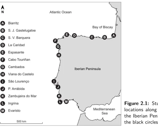
Biarritz A A Evaristo M M S. J. Gastelugatxe B B S. V. Barquera C C La Caridad D D Espasante E E Cabo Touriñan F F Cambados G G Viana do Castelo H H São Lourenço I I P. Arrábida J J Zambujeira do Mar K K Ingrina L L Bay of Biscay Mediterranean Sea Iberian Peninsula Atlantic Ocean N 500 km
Figure 2.1: Study area. Deployment
locations along the Atlantic coast of the Iberian Peninsula are depicted by the black circles.
these devices consist of a lithium battery powering the circuit board extracted from a DS1922L iButton (Dallas Semiconductor), embedded in a waterproof resin (3M Scotchcast 2130 Flame Retardant Compound), and placed inside an empty limpet shell (in the present work, from Patellaspp.). Two exposed wires penetrating the shell serve as contacts for logger programming and subsequent data retrieval. This design has previously been shown to accurately track the temperature profiles of live animals in the field, with errors smaller than the variability obtained by measuring the temperature of live animals a couple of meters apart (Lima and Wethey, 2009). Finally, because factory calibrations were lost when a Panasonic BR1255-1VC 3 V cell was used to replace the iButton battery (Lima and Wethey, 2009), assembled loggers were calibrated in the lab prior to field deployments (see Lima et al., 2010, for more details), restoring the original 0.5◦C logger accuracy.
Study area and deployment scheme
Intertidal temperatures were measured at 13 exposed or moderately exposed rocky shores along 1500 km of the Atlantic coast of the Iberian Peninsula (Fig.2.1). This coast encompasses a wide range of climatic and oceanographic conditions, such as a north to south cline in SST during the winter, and an alternation between warm and cold SST regions in summer. In this season, the strong upwelling off NW Iberia disrupts the latitudinal SST cline, making this region much cooler than either the NE or the SW Iberia (Lima et al., 2006; Wethey and Woodin,
2008;Berke et al., 2010).
At each location, biomimetic loggers were attached to steep rocky surfaces (i.e., with slopes between 60◦ and 90◦) with Z-Spar Splash Zone Compound (Kop-Coat Inc., Pittsburgh, Pennsylvania, USA) at three tidal heights, thus covering the entire vertical range inhabited
by limpets. ’Low-shore’ loggers were attached to the rock at the upper limit of the red algae belt, horizontally aligned with the lower distributional limit of P. ulyssiponensis Gmelin, 1791. ’Mid-shore’ loggers were deployed centred in the zone dominated by mussels (Mytilus sp.) and barnacles (Chthamalus spp.), amongst P. depressa Pennant, 1777 and P. vulgata Linnaeus, 1758. ’High-shore’ loggers were placed close to the lower limit of the black lichen Lichina pygmaea (Lightfoot) Agarth, 1821, at the upper limit of the distribution of P. vulgata and P. rustica. At each level, robolimpets were deployed in both north-facing (typically shaded) and south-facing (sun-exposed) rock surfaces. The combination of three heights and two orientations defined six microhabitats with potentially distinct thermal characteristics. Loggers were deployed in triplicate, for a total of 18 per shore. Robolimpets were programmed in the field with a laptop computer using a custom made communication cable (see Lima and Wethey, 2009) in association with the OneWireViewer software (www.maxim-ic.com). Loggers were programmed to record data at every 30 min, using a resolution of 0.5 ◦C in order to achieve long deployments (i.e., periods of 170 days). Thus, servicing occurred with a periodicity of approximately five months. At each visit to the shore, data was downloaded from working loggers, which were then reprogrammed, while malfunctioning loggers were replaced. Deployments were made between January 2008 and September 2009.
Data analysis
Data files were individually checked for any evidence of logger malfunction (e.g., in a few devices the internal clock stopped during the deployment), and discarded if necessary. Additionally, any interference due to logger handling in the field was eliminated by removing the first and the last 24 h of data from each logger. At each location, and for each deployment period x microhabitat combination, logged temperatures were averaged whenever data from multiple sensors was available. Thus, depending on the deployment period, the long-term thermal profiles could have been derived from 1–3 loggers (see Supp. Fig. 2.8 for the data coverage map). Finally, because tide cycles are not in phase across large geographical scales, an additional computation step was performed so that temperature values could be compared among locations. For example, in a one-to-one data point comparison, two identical thermal trajectories from distinct locations would be apparently different simply because they were 1h out-of-synchrony (which is, for instance, the average time difference in tide timing between SW France and SW Portugal). Thus, three different statistics were calculated (daily maximum, daily minimum and daily accumulated degrees-hour) to obtain single daily values which could then be compared across locations. In addition, to separately quantify thermal stress during aerial and submerged periods, statistics were also calculated for two data subsets (one consisting exclusively of temperature measurements two hours around local high tide, and a second one encompassing only those measurements taken two hours around local low tide). Both day-time and night-time tides were considered. Tidal elevation was obtained using the WTides software package (www.wtides.com).
Standard d eviation Correlation 0.0 0.5 1.0 1.5 2.0 0.0 0.5 1.0 1.5 2.0 0.6 0.4 0.8 0.9 0.99 0.5 1 2 1.5 rmse corr sd
Figure 2.2: Example of a Taylor
dia-gram. The colored circles represent dif-ferent temperature profiles being com-pared with a reference (depicted in black). The angular coordinate of a given point indicates the correlation be-tween that dataset and the reference (corr). Its radial distance from the reference shows its centred root mean square error (rmse), and the distance from the origin of the graph equals to the standard deviation (sd), normalized by the reference value.
Taylor diagrams were used to analyze similarity between thermal profiles. These diagrams have originally been devised for concisely summarizing the degree of correspondence between a suite of climatological model outputs and a known reference (Taylor, 2001). Taylor diagrams are particularly useful in evaluating multiple aspects of complex data series, since each graph shows a statistical summary of how well patterns match each other in terms of their correlation, their centred root mean square error (RMSE), and the ratio of their variances. When used separately, these three metrics provide quite incomplete estimates of the similarity between two datasets. For example, the RMSE is widely used to express the mean difference between two data series, but from a given RMSE alone it is impossible to understand if the two series are in phase or out-of-phase. This can be easily solved by providing a correlation coefficient along with the RMSE. Thus, two datasets are more similar if they have a small RMSE and a high correlation. Still, from those two metrics alone it is still not possible to determine whether two patterns have the same amplitude of variation, and so there is the need to consider the ratio of their variances (two patterns are more alike as the ratio of their variance approaches 1). Taylor diagrams show a visual representation of the three values at once and thus provide a quick but comprehensive summary of the degree of pattern correspondence. This method can also be used to summarize the relative skill of several datasets, identifying which one better resembles the reference.
A sample Taylor diagram can be found in Fig.2.2. Each dataset is represented by a point and its position in the plot quantifies how closely it matches the reference. The radial distance from the origin represents the amplitude of the temperature variation (standard deviation), normalized by the reference value. Thus, the closer a given point is to the radial line that crosses through the normalized reference value (sd = 1), the most similar that data is to the reference. The azimuthal angle of a particular point indicates its correlation to the reference. Thus, points closer to the bottom of the graph are generally more correlated with the reference.
Finally, the distance between a point and the reference shows the mean absolute difference between those datasets. Also here, points closer to the reference are more similar. For example, in Fig. 2.2, the hypothetical temperature trajectory represented by the red point has: (i) a correlation slightly higher than 0.9 in relation to the reference — as seen on the projection of the point in the curved right margin of the graph, (ii) an internal variability equivalent to approximately 1.5 times the standard deviation of the reference — as seen on the projection of the point on the horizontal axis, and finally, (iii) a mean absolute difference (RMSE) of 0.6◦C — as determined by its radial distance from the reference (black) point. In this example, it is also possible to see that even though the yellow and brown datasets have similar correlation coefficients (0.8) in relation to the reference, the variability of the data represented by the yellow point perfectly resembles the variability of the reference, while the brown dataset is much less variable. On average, data represented by the brown circle is also more different from the reference (~0.77 ◦C), when compared with the yellow dataset (~0.6 ◦C). Thus, the yellow point represents a data series more similar to the reference than the data series shown by the brown point. The green point has the worst correlation (approximately 0.5) and the worst RMSE (1.4 ◦C), but its variability in relation to the reference is similar to that of the red point. Still, and overall, the green point represents the dataset less similar to the reference. On the other hand, the blue circle shows the temperature profile with the highest similarity. It is the point that is closest to the reference, with a correlation of 0.99, a RMSE of less than 0.1 ◦C and a variability equivalent to the reference data.
A key analysis in the present work was to determine if the magnitude of the differences in body temperature was larger between opposing (sun versus shade) microhabitats at the same shore or, on the other hand, if it was greater across the latitudinal gradient for the same microhabitat. Thus, using a single Taylor diagram, each microhabitat (e.g., Biarritz mid-shore, sun-exposed) was directly compared with the opposing microhabitat from the same shore (Biarritz mid-shore, shade) and with the same microhabitat from the remaining shores (mid-shore, sun-exposed in all other locations). All data manipulation and subsequent analyses were done in R 2.11 (R Development Core Team, 2010), and Taylor plots were produced using the plotrix package (Lemon,2006) for R.
2.1.4
Results
The data coverage map is shown in Supp. Fig. 2.8. Despite some sporadic logger failures, temperature data was available for most microhabitats throughout the deployment period. Simultaneous data gaps (as happened in the beginning of 2009 across most locations) were caused by loggers’ memory limitations. Apart from that, the few cases of complete data loss across an entire microhabitat were almost invariably caused by deliberated logger destruction by beach combers or by fishermen harvesting intertidal gastropods. Generally, individual profiles were dominated by two main sources of variability. On one hand, all robolimpets displayed the
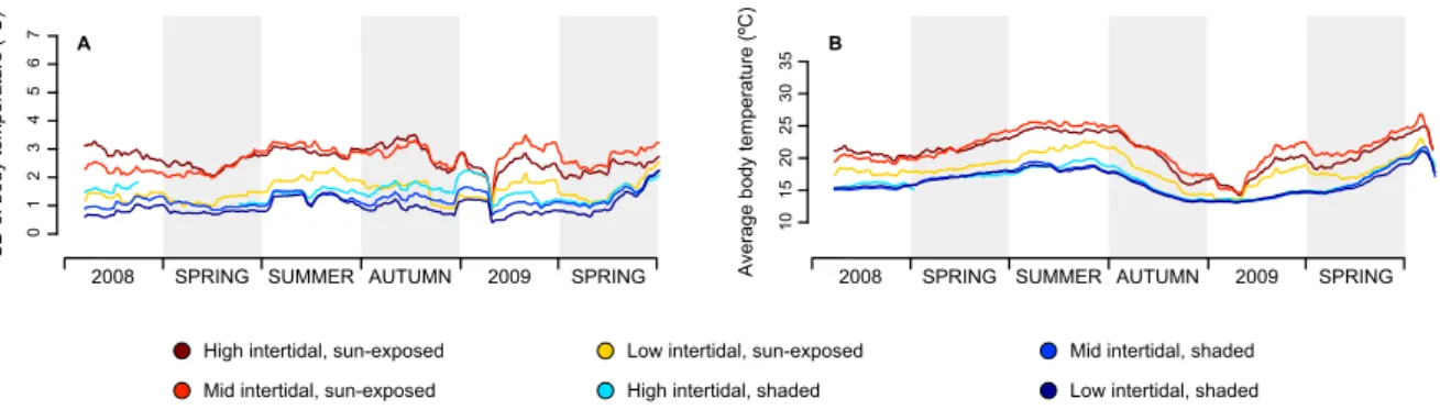
High intertidal, sun-exposed Mid intertidal, sun-exposed Low intertidal, sun-exposed
High intertidal, shaded Mid intertidal, shaded Low intertidal, shaded
2008 SPRING SUMMER AUTUMN 2009 SPRING SUMMER
Body temperature (ºC) 0 10 20 30 40 0 10 20 30 40 0 10 20 30 40 0 10 20 30 40 0 10 20 30 40 0 10 20 30 40 0 10 20 30
40 2008 SPRING SUMMER AUTUMN 2009 SPRING SUMMER
0 10 20 30 40 0 10 20 30 40 0 10 20 30 40 0 10 20 30 40 0 10 20 30 40 0 10 20 30 40 A (Biarritz) B (S. J. Gastelugatxe) C (S. V. Barquera) D (La Caridad) E (Espasante) F (C. Touriñan) G (Cambados) H (V. Castelo) I (S. Lourenço) J (P. Arrábida) K (Zambujeira) L (Ingrina) M (Evaristo)
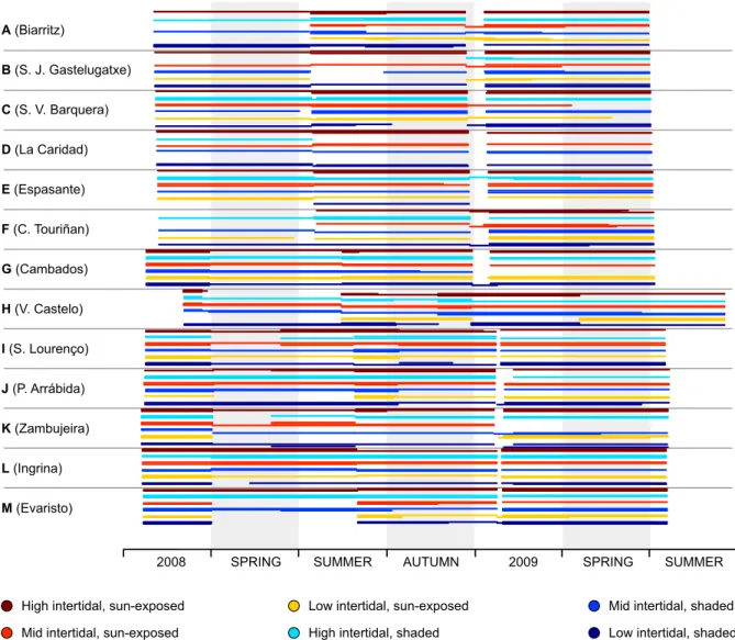
Figure 2.3: Body temperature profiles obtained by robolimpets deployed at different microhabitats
(depicted by the different line colors), within the 13 sampled locations, ordered from NE to SW Iberia (letters A–M, see also Fig. 2.1). Arrows indicate periods of upwelling relaxation off W Iberia.
typical seasonal pattern of sea water temperature variation, with the warmest temperatures during summer and the coldest temperatures during the winter (Fig. 2.3). Seasonality was also more evident along the northern coast of the Iberian Peninsula (Fig. 2.3A–E) in comparison with the upwelling-dominated western Iberia (Fig. 2.3F–M). On the other hand, high-frequency temperature oscillations, routinely exceeding 20 ◦C in less than 12 h (and even 30 ◦C on high shore loggers in summer) were clearly associated with tidal effects. High-frequency variability was especially remarkable in data from sun-exposed microhabitats, irrespectively of their height on the shore (see Fig.2.4A for an example and Supp. Fig. 2.9 for all locations).
2008 SPRING SUMMER AUTUMN 2009 SPRING
2008 SPRING SUMMER AUTUMN 2009 SPRING
High intertidal, sun-exposed Mid intertidal, sun-exposed
Low intertidal, sun-exposed High intertidal, shaded
Mid intertidal, shaded Low intertidal, shaded
B 10 15 20 25 30 35
Average body temperature (ºC)
A 0 1 2 3 4 5 6 7 SD of body temperature (ºC)
Figure 2.4: 30-day rolling average of standard variation (SD) of temperature profiles (A), and 30-day
rolling average of daily temperature maxima (B) for São Lourenço, in W Iberia.
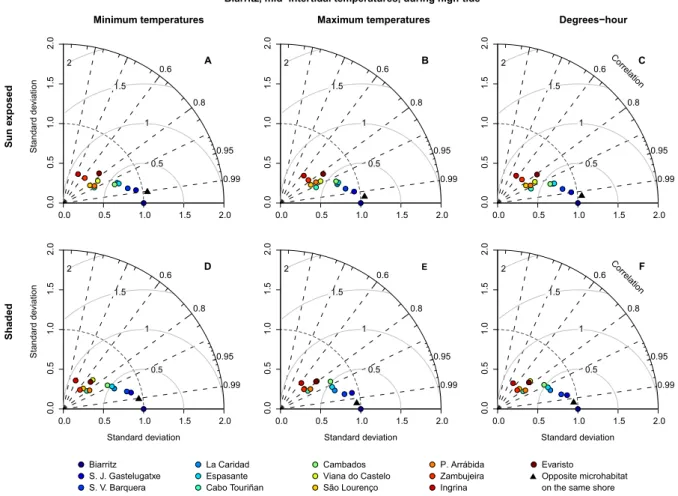
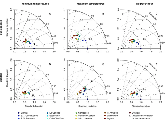
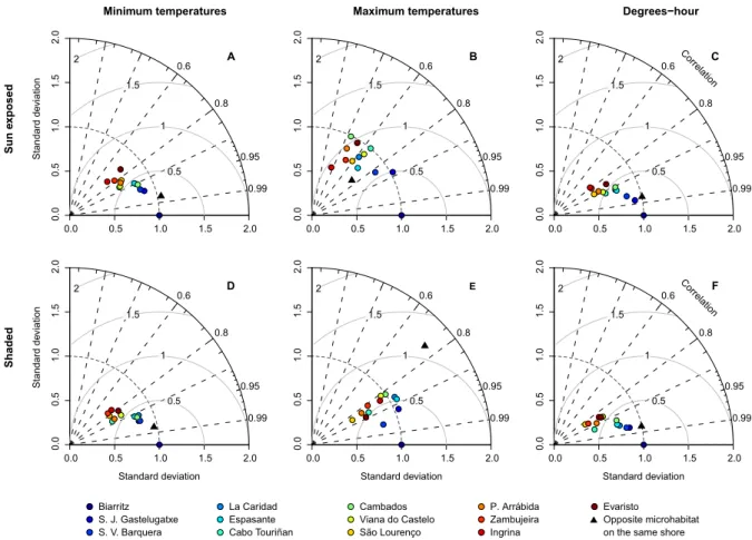
During low tide, sun-exposed robolimpets reached much higher maximum temperatures than their counterparts attached to north-facing surfaces (see Fig. 2.4B for an example and Supp. Fig. 2.10 for all locations), despite the fact that they were at the same tidal height and horizontally separated by less than a couple of meters. This difference was visible year-round, although its magnitude varied between seasons and locations. Temperature trajectories also showed the alternation between spring and neap tides, with daily maxima regularly oscillating in periods of approximately two weeks. This was particularly visible at locations with weaker seasonal influence (e.g., Fig.2.3I,K). Taylor plots displayed analogous patterns across locations (the complete set of plots can be found at Supp. Fig. 2.11; a small subset is shown for the mid-intertidal at Biarritz in Figs. 2.5,2.6and2.7). In general, results showed that either (i) the reference microhabitat was more closely related to the opposing microhabitat in the same shore, or (ii) that differences between the sun-exposed and shaded microhabitats were large enough so that the same habitat in other geographical locations was more similar to the reference. The first outcome was observed in 93% of the analyses comparing body temperatures measured during high tide (e.g., Fig. 2.5) or in 80% of the analyses where only minimum temperatures were considered, regardless of the tidal cycle (e.g., Figs. 2.5A,D, 2.6A,D and2.7A,D). The latter minimum temperatures are a proxy for emersion during the night. Hence, both cases reflect conditions where temperature experienced by organisms is homogeneous throughout the habitat, being independent of the shore level or surface orientation. Additionally, in any of the aforementioned cases, a clear latitudinal pattern in likeliness was also observed, with locations geographically near showing higher similarity values (clustering) in the Taylor diagrams. The second outcome was observed in 91% of the analyses focusing on maximum body temperatures or on the sum of all degree-hours measured either during low tide (Fig. 2.6B,E,C,F) or in 70% of the analyses involving the whole tidal cycle (Fig.2.7B,E, and C,F). Thus, whenever the analyses encompassed periods of air exposure during the day, shaded microhabitats were consistently more similar to shaded microhabitats on any other location than to any sun-exposed microhabitat on the same shore.
Biarritz S. J. Gastelugatxe S. V. Barquera La Caridad Espasante Cabo Touriñan Cambados Viana do Castelo São Lourenço P. Arrábida Zambujeira Ingrina Evaristo Opposite microhabitat on the same shore
Minimum temperatures
Standard d
eviation
Maximum temperatures Degrees−hour
Correlation
Standard deviation
Standard d
eviation
Standard deviation Standard deviation
Correlation Sun exposed Shaded 0.0 0.5 1.0 1.5 2.0 0.0 0.5 1.0 1.5 2.0 0.6 0.8 0.95 0.99 A 0.0 0.5 1.0 1.5 2.0 0.0 0.5 1.0 1.5 2.0 0.6 0.8 0.95 0.99 B 0.0 0.5 1.0 1.5 2.0 0.0 0.5 1.0 1.5 2.0 0.6 0.8 0.95 0.99 C 0.0 0.5 1.0 1.5 2.0 0.0 0.5 1.0 1.5 2.0 0.6 0.8 0.95 0.99 D 0.0 0.5 1.0 1.5 2.0 0.0 0.5 1.0 1.5 2.0 0.6 0.8 0.95 0.99 E 0.0 0.5 1.0 1.5 2.0 0.0 0.5 1.0 1.5 2.0 0.6 0.8 0.95 0.99 F 0.5 1 1.5 2 0.5 1 1.5 2 0.5 1 1.5 2 1 1.5 2 0.5 1 1.5 2 0.5 1 1.5 2
Biarritz, mid−intertidal temperatures, during high-tide
Figure 2.5: Taylor diagrams for robolimpet temperatures at Biarritz during a two-hour interval
around high tide. The radial distance from the origin represents the amplitude of temperature variation (standard deviation). The azimuthal angle depicts the correlation coefficient between the reference and the remaining microhabitats, while their RMSE is shown by the concentric lines centred on the reference.
2.1.5
Discussion
This work provided the first long-term series of intertidal animals’ body temperatures in a range of microhabitats, obtained by means of standardized methods, across a large geographical area. Overall, at each sampled location, maximum daily body temperatures were frequently associated with day-time emersions, while low peaks were linked to radiative and evaporative cooling during nocturnal low tides (seeDenny and Harley,2006;Gilman et al.,2006). Moreover, stable, overlapping temperature trajectories among different microhabitats corresponded to periods of logger immersion at high tide (hence reaching thermal equilibrium with sea water). Even though daily body temperature peaks during low tide have already been described for several intertidal animals (e.g.,Denny and Harley,2006; Szathmary et al., 2009; Jones et al.,2010) and algae (Pearson et al., 2009), data from the present work showed that even low-shore organisms are periodically exposed to temperatures exceeding 30◦C. Unexpectedly, these values were routinely experienced even at the northernmost locations (e.g., Fig. 2.3A). The most relevant finding of the present study is that the pervasive difference in temperature trajectories between
sun-Biarritz S. J. Gastelugatxe S. V. Barquera La Caridad Espasante Cabo Touriñan Cambados Viana do Castelo São Lourenço P. Arrábida Zambujeira Ingrina Evaristo Opposite microhabitat on the same shore
Minimum temperatures
Standard d
eviation
Maximum temperatures Degrees−hour
Correlation
Standard deviation
Standard d
eviation
Standard deviation Standard deviation
Correlation Sun exposed Shaded 0.0 0.5 1.0 1.5 2.0 0.0 0.5 1.0 1.5 2.0 0.6 0.8 0.95 0.99 A 0.0 0.5 1.0 1.5 2.0 0.0 0.5 1.0 1.5 2.0 0.6 0.8 0.95 0.99 B 0.0 0.5 1.0 1.5 2.0 0.0 0.5 1.0 1.5 2.0 0.6 0.8 0.95 0.99 C 0.0 0.5 1.0 1.5 2.0 0.0 0.5 1.0 1.5 2.0 0.6 0.8 0.95 D 0.99 0.0 0.5 1.0 1.5 2.0 0.0 0.5 1.0 1.5 2.0 0.6 0.8 0.95 0.99 E 0.0 0.5 1.0 1.5 2.0 0.0 0.5 1.0 1.5 2.0 0.6 0.8 0.95 0.99 F 0.5 1 1.5 2 0.5 1 1.5 2 0.5 1 1.5 2 1 1.5 2 0.5 1 1.5 2 0.5 1 1.5 2
Biarritz, mid−intertidal temperatures, during low-tide
Figure 2.6: Taylor diagrams for robolimpet temperatures at Biarritz during a two-hour interval
around low tide. The radial distance from the origin represents the amplitude of temperature variation (standard deviation). The azimuthal angle depicts the correlation coefficient between the reference and the remaining microhabitats, while their RMSE is shown by the concentric lines centred on the reference.
exposed and shaded microhabitats may be a common feature of intertidal habitats, even across large geographical areas subjected to heterogeneous climatic and oceanographic conditions. Sunny versus shaded differences were consistently larger than the variability associated with the seasons, with shore-specific characteristics (topography, orientation, wave exposure, etc.) and with shore level (Fig. 2.3). Regarding the similarity patterns found during high tide, robolimpets’ thermal trajectories were clearly driven by sea temperature, which suppressed any differences attained during emersions. In this scenario, similarities were typically higher between areas that were spatially closer (the opposite surfaces of the same rocky outcrop), decreasing consistently as geographical distance increased. Temperature profiles exhibited a more pronounced seasonality in the N and NE Iberia, when compared with the western coast. While the oceanographic conditions in the Bay of Biscay are in general characterized by a weak upwelling and low turbulence, particularly during the warm season (Borja et al., 1996,
2008; Bode et al., 2009), in the western Iberia coastal temperatures are strongly influenced by the development of an upwelling system during summer and early autumn months (Peliz et al.,2002;Lemos and Pires,2004;Lemos and Sansó,2006;Relvas et al.,2007). Interestingly,
Biarritz S. J. Gastelugatxe S. V. Barquera La Caridad Espasante Cabo Touriñan Cambados Viana do Castelo São Lourenço P. Arrábida Zambujeira Ingrina Evaristo Opposite microhabitat on the same shore
Minimum temperatures
Standard d
eviation
Maximum temperatures Degrees−hour
Correlation
Standard deviation
Standard d
eviation
Standard deviation Standard deviation
Correlation Sun exposed Shaded 0.0 0.5 1.0 1.5 2.0 0.0 0.5 1.0 1.5 2.0 0.6 0.8 0.95 0.99 A 0.0 0.5 1.0 1.5 2.0 0.0 0.5 1.0 1.5 2.0 0.6 0.8 0.95 0.99 B 0.0 0.5 1.0 1.5 2.0 0.0 0.5 1.0 1.5 2.0 0.6 0.8 0.95 0.99 C 0.0 0.5 1.0 1.5 2.0 0.0 0.5 1.0 1.5 2.0 0.6 0.8 0.95 0.99 D 0.0 0.5 1.0 1.5 2.0 0.0 0.5 1.0 1.5 2.0 0.6 0.8 0.95 0.99 E 0.0 0.5 1.0 1.5 2.0 0.0 0.5 1.0 1.5 2.0 0.6 0.8 0.95 0.99 F 0.5 1 1.5 2 0.5 1 1.5 2 0.5 1 1.5 2 1 1.5 2 0.5 1 1.5 2 0.5 1 1.5 2
Biarritz, mid−intertidal temperatures, during the entire tide
Figure 2.7: Taylor diagrams for robolimpet temperatures at Biarritz during the entire tide. The
radial distance from the origin represents the amplitude of temperature variation (standard deviation). The azimuthal angle depicts the correlation coefficient between the reference and the remaining microhabitats, while their RMSE is shown by the concentric lines centred on the reference.
present results suggest that the cooling influence of the upwelling system propagates into the innermost coastal waters, driving, to a great extent, body temperatures of intertidal animals (see for instance how temperature profiles south of Viana do Castelo in Fig. 2.3H–L are more leveled than in the northernmost locations). Even higher-frequency and smaller-scale events such as the intermittent upwelling relaxation which is characteristic of this region (Moncoiffe et al., 2000;Relvas et al., 2007) influenced logged temperatures (e.g., rapid increases in sea temperature registered at Viana do Castelo and S. Lourenço in the summers of 2008 and 2009 — please see arrows in Fig.2.3H,I). The present findings emphasize the importance of analyzing temperature variability at scales relevant to the organisms, since the usage of SST derived from remote sensed data to model the distribution of intertidal species (e.g., Poloczanska et al., 2008) may be missing key environmental features (Helmuth et al., 2010). Results clearly show that other factors than SST play a much stronger role in determining the body temperatures of these organisms, even at lower levels on the shore. Hence, even the organisms that are only exposed during extreme low tides can be routinely subjected to potentially stressful conditions. Overall, the observed temperature variability may explain the weak correlations
found in many studies modeling the distribution of intertidal species using SST data (e.g.,
Lima et al., 2007b), which negatively impacts attempts of forecasting distributional changes in response to predicted climate warming. Conversely, habitat heterogeneity as determined by surface orientation and, to a lesser extent, height on the shore may provide thermal refugia allowing species to occupy habitats apparently inhospitable when considering only average temperatures. This may be important for understanding range shifts contrary to global warming predictions (e.g.,Lima et al.,2007a,2009;Hilbish et al.,2010). In the specific case of intertidal limpets, the present results may be used for establishing theoretical frameworks upon which hypotheses can be formulated and tested. For example, future studies could try to find whether different body temperatures observed in association with sunny/shaded microhabitats translate into different levels of physiological stress. It would also be interesting to understand if limpets take advantage of the small-scale thermal differences in their habitat to regulate their body temperature according to their physiological requirements (e.g., by seeking shade in response to intense solar radiation). There is evidence that the more northern limpet species (e.g., Patella vulgata) seek shade under fucoid clumps, whilst other species (e.g., Patella depressa, a southern species) do not (Moore et al., 2007). On the other hand, biomimetic loggers (robolimpets) could be used in association with experimental manipulations in the field to find if (and to which extent) limpet grazing is determined by the thermal environment. That information is important not only for the study of the ecology, physiology and behavior of these gastropods but also for understanding the network of ecological relations among intertidal organisms, given the broad importance of limpet grazing in intertidal systems (e.g., Hawkins and Hartnoll,
1983; Coleman et al., 2006;Jenkins et al.,2008). These results are remarkable in that they show that thermal differences between microhabitats separated by only a few meters on a shore (sunny versus shaded microhabitats) are more different than sites hundreds of km apart. It has long been appreciated that there are strong physical gradients between the high and low tide-marks on shores, but differences between sunny and shaded microhabitats have been less well understood, and the data presented here indicated that they overwhelm differences between shore levels. These results suggest that thermal heterogeneity within habitats must be fully understood in order to interpret patterns of biogeographic response to climate change.
2.1.6
Acknowledgements
The authors thank Nuno Queiroz, Lara Sousa, Raquel Xavier, Sérgia Velho, Pedro Ribeiro and Jerry Hilbish for their help during fieldwork and for their insightful suggestions. Fund-ing was provided by grants from NOAA (NA04NOS4780264), NASA (NNG04GE43G and NNX07AF20G), National Science Foundation (OCE1039513) and Fundação para a Ciência e a Tecnologia (PTDC/MAR/099391/2008 and SFRH/BPD/34932/2007).
2.1.7
Supplementary data
2008 SPRING SUMMER AUTUMN 2009 SPRING SUMMER
High intertidal, sun-exposed Mid intertidal, sun-exposed
Low intertidal, sun-exposed High intertidal, shaded
Mid intertidal, shaded Low intertidal, shaded
H (V. Castelo) I (S. Lourenço) J (P. Arrábida) K (Zambujeira) L (Ingrina) M (Evaristo) A (Biarritz) B (S. J. Gastelugatxe) C (S. V. Barquera) D (La Caridad) E (Espasante) F (C. Touriñan) G (Cambados)
Figure 2.8: Data coverage map showing the number of operational robolimpets at a given time
(thickness of line) on the 6 intertidal microhabitats of the 13 sampled shores. Shores are arranged from ordered from NE (top) to SW Iberia (bottom). Each line color represents a different intertidal microhabitat.
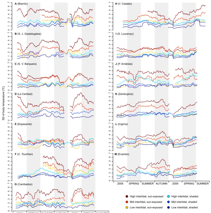
SD of body temperature (ºC) A B C D E F G H M
High intertidal, sun-exposed Mid intertidal, sun-exposed Low intertidal, sun-exposed
High intertidal, shaded Mid intertidal, shaded Low intertidal, shaded SUMMER
2008 SPRING SUMMER AUTUMN 2009 SPRING SUMMER
2008 SPRING SUMMER AUTUMN 2009 SPRING
(Biarritz) (S. J. Gastelugatxe) (S. V. Barquera) (La Caridad) (Espasante) (C. Touriñan) (Cambados) (V. Castelo) (S. Lourenço) (P. Arrábida) (Zambujeira) (Ingrina) (Evaristo) I J K L 0 1 2 3 4 5 6 7 0 1 2 3 4 5 6 7 0 1 2 3 4 5 6 7 0 1 2 3 4 5 6 7 0 1 2 3 4 5 6 7 0 1 2 3 4 5 6 7 0 1 2 3 4 5 6 7 0 1 2 3 4 5 6 7 0 1 2 3 4 5 6 7 0 1 2 3 4 5 6 7 0 1 2 3 4 5 6 7 0 1 2 3 4 5 6 7 0 1 2 3 4 5 6 7
Figure 2.9: 30-day rolling average of standard variation (SD) of temperature profiles within the 13
Average body temperature (ºC) A B C D E F G H M
High intertidal, sun-exposed Mid intertidal, sun-exposed Low intertidal, sun-exposed
High intertidal, shaded Mid intertidal, shaded Low intertidal, shaded SUMMER
2008 SPRING SUMMER AUTUMN 2009 SPRING SUMMER
2008 SPRING SUMMER AUTUMN 2009 SPRING
(Biarritz) (S. J. Gastelugatxe) (S. V. Barquera) (La Caridad) (Espasante) (C. Touriñan) (Cambados) (V. Castelo) (S. Lourenço) (P. Arrábida) (Zambujeira) (Ingrina) (Evaristo) I J K L 10 15 20 25 30 35 10 15 20 25 30 35 10 15 20 25 30 35 10 15 20 25 30 35 10 15 20 25 30 35 10 15 20 25 30 35 10 15 20 25 30 35 10 15 20 25 30 35 10 15 20 25 30 35 10 15 20 25 30 35 10 15 20 25 30 35 10 15 20 25 30 35 10 15 20 25 30 35
Figure 2.10: 30-day rolling average of daily temperature maxima of temperature profiles within the
Biarritz, low−intertidal temperatures, during high−tide Sun exposed Minimum temperatures Standard deviation Standard d eviation 0.0 0.5 1.0 1.5 2.0 0.0 0.5 1.0 1.5 2.0 0.5 1 1.5 2 ● 0.2 0.4 0.6 0.8 0.95 0.99 Correlation ● ●● ● ● ● ● ●●● ● ● A Maximum temperatures Standard deviation Standard d eviation 0.0 0.5 1.0 1.5 2.0 0.0 0.5 1.0 1.5 2.0 0.5 1 1.5 2 ● 0.2 0.4 0.6 0.8 0.95 0.99 Correlation ● ● ● ● ● ● ● ●●● ● ● B Degrees−hour Standard deviation Standard d eviation 0.0 0.5 1.0 1.5 2.0 0.0 0.5 1.0 1.5 2.0 0.5 1 1.5 2 ● 0.2 0.4 0.6 0.8 0.95 0.99 Correlation ● ● ● ● ● ● ● ●●● ● ● C Shaded Standard deviation Standard d eviation 0.0 0.5 1.0 1.5 2.0 0.0 0.5 1.0 1.5 2.0 0.5 1 1.5 2 ● 0.2 0.4 0.6 0.8 0.95 0.99 Correlation ● ● ● ●● ●● ● ●● ● ● ● D Standard deviation Standard d eviation 0.0 0.5 1.0 1.5 2.0 0.0 0.5 1.0 1.5 2.0 0.5 1 1.5 2 ● 0.2 0.4 0.6 0.8 0.95 0.99 Correlation ● ● ● ● ● ●● ● ●● ● ● ● E Standard deviation Standard d eviation 0.0 0.5 1.0 1.5 2.0 0.0 0.5 1.0 1.5 2.0 0.5 1 1.5 2 ● 0.2 0.4 0.6 0.8 0.95 0.99 Correlation ● ● ● ●● ●● ● ●● ● ● ● F ● ● ● Biarritz S. J. Gastelugatxe S. V. Barquera ● ● ● La Caridad Espasante Cabo Touriñan ● ● ● Cambados Viana do Castelo São Lourenço ● ● ● P. Arrábida Zambujeira Ingrina ● Evaristo Opposite microhabitat on the same shore
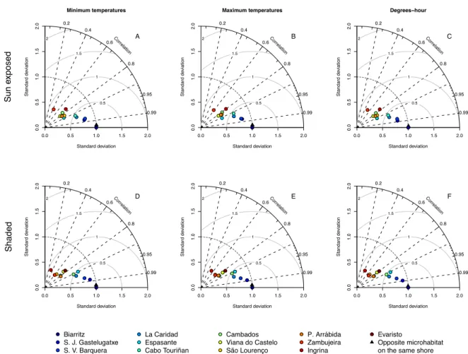
Figure 2.11: Taylor diagrams for robolimpet temperatures measured within the 13 sampled locations,
during (i) a two-hour interval around high tide, (ii) a two-hour interval around low tide and (iii) the entire tide, at three intertidal levels (low-, mid- and high-intertidal). On each diagram, the radial distance from the origin represents the amplitude of temperature variation (standard deviation). The azimuthal angle depicts the correlation coefficient between the reference and the remaining microhabitats, while their RMSE is shown by the concentric lines centred on the reference. The full set of 114 panels can be found online at doi:10.1016/j.jembe.2011.02.010.