Todos os direitos reservados.
É proibida a reprodução parcial ou integral do conteúdo
deste documento por qualquer meio de distribuição, digital ou
impresso, sem a expressa autorização do
REAP ou de seu autor.
Real Rigidities and the Cross-Sectional
Distribution of Price
Stickiness: Evidence from Micro and Macro Data
Combined
Carlos Carvalho
Niels Arne Dam
Jae Won Lee
Real Rigidities and the Cross-Sectional Distribution of Price
Stickiness: Evidence from Micro and Macro Data Combined
Carlos Carvalho
Niels Arne Dam
Jae Won Lee
Carlos Viana de Carvalho
Pontifícia Universidade Católica do Rio de Janeiro (PUC-Rio)
Departamento de Economia
Rua Marquês de São Vicente, nº 225
Gávea
22451-900 - Rio de Janeiro, RJ - Brasil
[email protected]
Niels Arne Dam
Danmarks Nationalbank
Jae Won Lee
Real Rigidities and the Cross-Sectional Distribution of Price
Stickiness: Evidence from Micro and Macro Data Combined
Carlos Carvalho PUC-Rio
Niels Arne Dam Danmarks Nationalbank
Jae Won Lee Seoul National University
December, 2014
Abstract
We use a standard sticky-price model to provide evidence on three mechanisms that can reconcile somewhat frequent price changes with large and persistent real e¤ects of monetary shocks. To that end, we estimate a semi-structural model for the U.S. economy that allows for varying degrees of real rigidities, and cross-sectional heterogeneity in price stickiness. The model can extract some information about these two features of the economy from aggregate data, and discriminate between di¤erent distributions of price stickiness. Hence it can also speak to the debate about the role of sales and other temporary price changes in shaping the e¤ects of monetary policy. Employing a Bayesian approach, we combine macroeconomic time-series data with information about empirical distributions of price stickiness derived from micro price data for the U.S. economy. Our estimates point to the presence of both large real rigidities and an important degree of heterogeneity in price stickiness. Moreover, cross-sectional distributions of price stickiness that factor out sales improve the empirical …t of the model. Our results suggest that bridging the gap between micro and macro evidence on nominal price rigidity may require the combination of several mechanisms.
JEL classi…cation codes: E10, E30
Keywords: real rigidities, heterogeneity in price stickiness, sales, regular prices, micro data, macro
data, Bayesian estimation
1
Introduction
Our understanding of the real e¤ects of monetary policy hinges, to a large extent, on the existence of some degree of nominal price rigidity. In the decade since the publication of the seminal Bils and Klenow (2004) paper, the availability of large amounts of micro price data has rekindled interest in this area, and allowed us to make progress. Yet, estimates of the extent of nominal price stickiness based on microeconomic data versus those based on aggregate data usually produce a con‡icting picture.
According to Klenow and Malin’s (2011) survey of the empirical literature based on micro data, prices change, on average, at least once a year – somewhat more often than we thought was the case prior to Bils and Klenow (2004). In contrast, making sense of estimates of the response of the aggregate price level to monetary shocks (from dynamic stochastic general equilibrium – DSGE – models, or vector autoregressions) requires much less frequent price adjustments.1
If nominal price rigidities are to continue to be the leading explanation for why monetary policy has large and persistent real e¤ects, it is important that we deepen our understanding of mechanisms that can narrow the gap between the evidence of somewhat ‡exible individual prices and relatively sluggish aggregate prices – i.e., mechanisms that can produce a large “contract multiplier”. If prices change frequently and each and every price change contributes to fully o¤set nominal disturbances, then nominal price rigidity cannot be the source of large and persistent monetary non-neutralities. Hence, a large contract multiplier requires that price adjustments, somehow, fail to perfectly neutralize monetary innovations.
In this paper, our goal is to contribute to bridge the gap between micro and macro evidence on the extent of nominal price rigidity. To that end, we estimate a standard macroeconomic model of price setting, and use it to speak to three mechanisms that can boost the contract multiplier. The …rst such mechanism are so-called “real rigidities”, in the sense of Ball and Romer (1990). Large real rigidities reduce the sensitivity of individual prices to aggregate demand conditions, and thus serve as a source of endogenous persistence: for any given degree of price stickiness, partial adjustment of individual prices makes for a sluggish response of the aggregate price level to monetary shocks.
The other two mechanisms are motivated by the empirical evidence uncovered since Bils and Klenow (2004), and subsequent theoretical literature. Cross-sectional heterogeneity in price rigidity, to the extent documented in the micro data, can lead to much larger monetary non-neutralities than the average frequency of price changes would imply (Carvalho 2006, Nakamura and Steinsson 2010). The reason is that, while recurrent price changes by …rms in more ‡exible sectors do not contribute as much
to o¤set monetary shocks, they do count for the frequency of price adjustment.2 Heterogeneity can
become an even more powerful mechanism when coupled with strategic complementarities in pricing decisions. In those circumstances, …rms in the more sticky sectors become disproportionately important in shaping aggregate dynamics (relative to their sectoral weight), through their in‡uence on pricing decisions of …rms that change prices more frequently (Carvalho 2006).3
The third mechanism is the presence of sales and other temporary price changes. Guimaraes and Sheedy (2011) and Kehoe and Midrigan (2014) show that such price changes may help reconcile frequent micro adjustments with a sluggish aggregate price response to nominal disturbances.4 A basic intuition
for their results is that temporary price changes fail to o¤set monetary shocks well, since these shocks tend to induce permanent changes in the level of prices.5
We estimate a macroeconomic model that, while relatively standard, can provide some information about the three aforementioned mechanisms based on aggregate data. The price-setting block of the model is a multi-sector sticky-price economy that allows for heterogeneity in price stickiness, and can feature strategic complementarity or substitutability in pricing decisions. The remaining equations specify exogenous stochastic processes that drive …rms’ frictionless optimal prices. They provide the model with some ‡exibility to perform in empirical terms, and thus allow us to focus on the objects of interest in the price-setting block of the economy. Hence, we refer to our model as “semi-structural”.6
We show that, at least in theory, the model is able to separately identify real and nominal rigidities, and tell apart economies with homogenous from those with heterogeneous price stickiness – based on aggregate data only. The model can also discriminate between di¤erent (non-degenerate) distributions of price rigidity, providing information on which one helps explain aggregate dynamics better. Hence, at least in theory, our analysis can also speak to the debate about how to treat temporary sales in micro price data.
2Carvalho and Schwartzman (2014) show how this intuition can be formalized in terms of a “selection e¤ect” relative
to the timing of price changes, which arises in the class of time-dependent pricing models.
3Nakamura and Steinsson (2010) conclude that this interaction is not important in their calibrated menu-cost model.
4Coibion et al. (2014) provide evidence that sales are essentially acyclical – which is consistent with the models in
Guimaraes and Sheedy (2011) and Kehoe and Midrigan (2014). Kryvtsov and Vincent (2014), on the other hand, argue that sales do not help reconcile micro and macro evidence on price rigidity. They document a large degree of cyclicality of sales in the U.K. micro data, and develop a model that can explain their …ndings. In bad times, consumers intensify search for bargain prices and …rms increase the frequency of sales. This “complementarity” between search e¤ort and sales frequency breaks down the strategic substitutability of sales that would otherwise arise (as in Guimaraes and Sheedy 2011), and leads to cyclical sales.
5Information frictions can also lead to large contract multipliers. Not surprisingly, that literature picked up steam after
the empirical literature based on micro price data ‡ourished. Classic contributions include Caballero (1989), Reis (2006), and Ma´ckowiak and Wiederholt (2009), who obtain large monetary non-neutralities in models with information frictions in which prices change continuously. More recently, Bonomo, Carvalho, Garcia, and Malta (2014) obtain a large contract multiplier in an estimated model with menu costs and partially costly information.
6Several earlier papers in the literature combine structural equations with empirical speci…cations for other parts of
Identi…cation of those features of price setting based on aggregate data is possible in our model because sectors that di¤er in price stickiness have di¤erent implications for the response of the macro-economy to shocks at di¤erent frequencies. In particular, sectors where prices are more sticky are relatively more important in determining the low-frequency response to shocks; and vice-versa for more ‡exible sectors. These di¤erences provide information about the cross-sectional distribution of price stickiness. Finally, separate identi…cation of real and nominal rigidities comes from the way in which the aggregate price level depends on its own lags vis-a-vis lags of exogenous drivers of …rms’ frictionless optimal prices.
While our approach requires that we learn something about the mechanisms of interest from aggre-gate data, we argue that a more promising direction is to combine those data with information about the empirical cross-sectional distribution of price stickiness derived from micro price data.
In their favor, the micro data have the millions of observations used to compute measures of price rigidity. They also allow us to estimate separate distributions of price rigidity, with and without sales. Hence, on these grounds, one could imagine imposing alternative empirical distributions of price rigidity derived from micro data (e.g., with and without sales), estimating the other parameters of the model – in particular, the parameter associated with real rigidities – and comparing the performance of di¤erent estimated models in terms of …t and other dimensions of interest.
However, treating the estimates derived from micro data as the true “population moments” that matter for aggregate dynamics is not appropriate, in our view. First, it is possible that some price adjustments do not convey as much information about changes in macroeconomic conditions as others do. While this possibility is at the core of the debate about whether or not to exclude sales from price setting statistics for macro purposes, the argument applies more generally – for example, it also applies to the literature on price setting under information frictions. In that case, macro-based estimates should convey useful information about the price changes that do matter for aggregate dynamics. Second, and not less importantly, Eichenbaum et al. (2014) show that the BLS micro data underlying the CPI are plagued with measurement problems when it comes to computing statistics based on individual price changes. While Eichenbaum et al. (2014) focus on pitfalls involved in estimating the distribution of the size of price changes, the problems they document certainly add measurement error to available estimates of the cross-sectional distribution of price stickiness that use that data (e.g., Bils and Klenow 2004, Nakamura and Steinsson 2008, Klenow and Kryvtsov 2008).
information that they contain.
To strike a balance between extracting information from aggregate data and exploring what we know based on the micro data, we employ a full-information Bayesian approach. We use aggregate (time-series) data on nominal and real Gross Domestic Product (GDP) as observables, and incorporate the microeconomic information about the cross-sectional distribution of price stickiness through our prior on the model parameters that govern that distribution. Speci…cally, we parameterize that prior in a way that easily allows us to relate its moments to the analogous moments of empirical distributions of price stickiness. We focus on two empirical distributions: one that takes into account all price changes, including sales (derived from Bils and Klenow 2004); and another, based on “regular” price changes, that excludes sales and product substitutions (derived from Nakamura and Steinsson 2008).
We summarize our …ndings as follows. The estimated models can discriminate quite sharply between economies with heterogeneity in price stickiness and their homogeneous-…rms counterparts. They also point to the existence of large real rigidities, which induce strong strategic complementarities in price setting.
Turning to the cross-sectional distribution of price rigidity, the information extracted from aggre-gate data accords quite well with the micro data. Speci…cally, the distribution estimated under an uninformative (“‡at”) prior has a correlation of 0.43 with the distribution that leaves sales in (Bils and Klenow 2004), and a correlation of 0.63 with the distribution that excludes sales and product substitu-tions (Nakamura and Steinsson 2008). Moreover, a formal statistical comparison between models with informative priors based on those two cross-sectional distributions provides some additional evidence in favor of the distribution based on regular prices.
Altogether, our results suggest that all three mechanisms that can boost the contract multiplier might have a role to play in our understanding of the e¤ects of monetary policy.
1.1 Brief literature review
Our work is related to the literature that emphasizes the importance of heterogeneity in price rigidity for aggregate dynamics. However, our focus di¤ers from that of existing papers. Most of the latter focus on the role of heterogeneity in boosting the contract multiplier in calibrated models (e.g., Carvalho 2006, Carvalho and Schwartzman 2008, Nakamura and Steinsson 2010, Carvalho and Nechio 2010, Dixon and Kara 2011). These papers do not address the question of whether such heterogeneity does in fact help sticky-price models …t the data better according to formal statistical criteria.
estimation methods that do not account for heterogeneity. They rely on sectoral data for France, and …nd that the results based on estimators that allow for heterogeneity are more in line with the available microeconomic evidence on price rigidity. Lee (2009) and Bouakez et al. (2009) estimate multi-sector DSGE models with heterogeneity in price rigidity using aggregate and sectoral data. They also …nd results that are more in line with the microeconomic evidence than the versions of their models that impose the same degree of price rigidity for all sectors.7 Taylor (1993) provides estimates of the
distribution of the duration of wage contracts in various countries inferred solely from aggregate data, while Guerrieri (2006) provides estimates of the distribution of the duration of price spells in the U.S. based on aggregate data. Both models feature ex-post rather than ex-ante heterogeneity in nominal rigidities, as is the case in our model.8 Coenen et al. (2007) estimate a model with (limited) ex-ante
heterogeneity inprice contractsusing only aggregate data. They focus on the estimate of the Ball-Romer
index of real rigidities and on the average duration of contracts implied by their estimates, which they emphasize is in line with the results in Bils and Klenow (2004).9
Jadresic (1999) is a precursor to some of the ideas in this paper. He estimates a model with ex-ante heterogeneous price spells using only aggregate data for the U.S. economy to study the joint dynamics of output and in‡ation. Similarly to our …ndings, his statistical results reject the assumption of identical …rms. Moreover, he discusses the intuition behind the source of identi…cation of the cross-sectional distribution of price rigidity from aggregate data in his model, which is the same as in our model. Despite these similarities, our paper di¤ers from Jadresic’s in several important dimensions. We use a di¤erent estimation method, and show the possibility of extracting information about the cross-sectional distribution of price rigidity from aggregate data in a more general context - in particular in the presence of pricing complementarities. Most importantly, the focus of our paper goes beyond assessing the empirical support for heterogeneity in price rigidity from aggregate data. We also investigate the similarities between our macro-based estimates and the available microeconomic evidence, and propose an approach to integrate the two sources of information on the distribution of price rigidity.
Finally, our results speak to the ongoing debate on the role of sales in macroeconomic models. That literature started out as a discussion about whether or not to exclude sales when computing price-setting statistics for macro purposes (Bils and Klenow 2004, Nakamura and Steinsson 2008, Klenow and Kryvtsov 2008). This initial debate was followed by a theoretical literature that provided
macro-7Bouakez et al. (2014) …nd similar results in an extension of their earlier paper to a larger number of sectors.
8Their frameworks are thus closer to the generalized time-dependent model of Dotsey et al. (1997) than to our model
with ex-ante heterogeneity.
9Their estimated model features indexation to an average of past in‡ation and a (non-zero) constant in‡ation objective.
economic models with sales and other temporary price changes (Guimaraes and Sheedy 2011, Kehoe and Midrigan 2014). More recently, the literature has focused on the cyclicality of sales and consumer behavior, both in theory and in the micro data (e.g., Coibion et al. 2014, Kryvtsov and Vincent 2014). We provide statistical evidence on the relative performance of macroeconomic models with di¤erent distributions of price rigidity that do and do not exclude sales (and product substitutions).
In Section 2 we present the semi-structural model and study the extent to which aggregate data contain information about the cross-sectional distribution of price stickiness and the parameter that controls the extent of real rigidities in the model. Section 3 describes our empirical methodology and data. In Section 4 we present our main results. We start with macro-based estimates obtained under an uninformative prior, assess the estimates against the empirical distributions from Bils and Klenow (2004) and Nakamura and Steinsson (2008), and perform model comparison with speci…cations that impose the same degree of price rigidity for all …rms. We then provide our estimates that incorporate information from the micro data, and perform model comparison with di¤erent prior distributions. Section 6 reports our robustness analysis, and discusses the performance of the estimated model in light of additional micro price facts. The last section concludes.
2
The semi-structural model
There is a continuum of monopolistically competitive …rms divided into K sectors that di¤er in the frequency of price changes. Firms are indexed by their sector, k 2 f1; :::; Kg, and by j 2 [0;1]. The distribution of …rms across sectors is summarized by a vector (!1; :::; !K) with !k >0; PKk=1!k = 1,
where !k gives the mass of …rms in sector k. Each …rm produces a unique variety of a consumption
good, and faces a demand that depends negatively on its relative price.
In any given period, pro…ts of …rm j from sector k (henceforth referred to as “…rm kj”) are given by:
t(k; j) =Pt(k; j)Yt(k; j) C(Yt(k; j); Yt; t);
wherePt(k; j) is the price charged by the …rm,Yt(k; j)is the quantity that it sells at the posted price
(determined by demand), andC(Yt(k; j); Yt; t)is the total cost of producing such quantity, which may
also depend on aggregate output Yt, and is subject to shocks ( t). We assume that the demand faced
by the …rm depends on its relative price Pt(k;j)
Pt , where Pt is the aggregate price level in the economy,
and on aggregate output. Thus, we write …rmkj’s pro…t as:
and make the usual assumption that is homogeneous of degree one in the …rst two arguments, and single-peaked at a strictly positive level ofPt(k; j) for any level of the other arguments.10
The aggregate price index combines sectoral price indices,Pt(k)’s, according to the sectoral weights,
!k’s:
Pt= fPt(k); !kgk=1;:::;K ;
where is an aggregator that is homogeneous of degree one in the Pt(k)’s. In turn, the sectoral
price indices are obtained by applying a symmetric, homogeneous-of-degree-one aggregator to prices charged by all …rms in each sector:
Pt(k) = fPt(k; j)gj2[0;1] :
We assume the speci…cation of staggered price setting inspired by Taylor (1979, 1980). Firms set prices that remain in place for a …xed number of periods. The latter is sector-speci…c, and we save on notation by assuming that …rms in sector k set prices for k periods. Thus, ! = (!1; :::; !K) fully
characterizes the cross-sectional distribution of price stickiness that we are interested in. Finally, across all sectors, adjustments are staggered uniformly over time.
Before we continue, a brief digression about the Taylor pricing model is in order. As will become clear, this model allows us to tell apart real rigidities from nominal rigidities, and to infer the cross-sectional distribution of price stickiness implied by aggregate data. Hence, it serves our purposes well. However, strictly speaking, that model is at odds with the microeconomic evidence on the duration of price spells. Klenow and Kryvtsov (2008), for example, provide evidence that the duration of individual price spells varies at thequote line level. However, this evidence does not invalidate the use of the Taylor
model for our purposes. In particular, in Section 5 we provide an alternative model in which the duration of price spells varies at the …rm level, and yet the aggregate behavior of the model is identical to the one presented here. The alternative model can match additional micro facts documented in the literature. Hence, it provides a cautionary note on attempts to test speci…c models of price setting by confronting them with descriptive micro price statistics. For ease of exposition, we proceed with the standard Taylor pricing speci…cation. But the reader should keep in mind that the aggregate implications that we are interested survive in models that can match the microeconomic evidence in many dimensions.
When setting its priceXt(k; j) at time t, given that it sets prices fork periods, …rmkj solves:
maxEt k 1
X
i=0
Qt;t+i Xt(k; j); Pt+i; Yt+i; t+i ;
whereQt;t+i is a (possibly stochastic) nominal discount factor. The …rst-order condition for the …rm’s
problem can be written as:
Et k 1
X
i=0
Qt;t+i
@ Xt(k; j); Pt+i; Yt+i; t+i
@Xt(k; j)
= 0: (1)
Note that all …rms from sectork that adjust prices at the same time choose a common price, which we denoteXt(k).11 Thus, for a …rmkj that adjusts at timet and setsXt(k), the prices charged from tto
t+k 1satisfy:
Pt+k 1(k; j) =Pt+k 2(k; j) =:::=Pt(k; j) =Xt(k):
Given the assumptions on price setting, and uniform staggering of price adjustments, with an abuse of notation sectoral prices can be expressed as:
Pt(k) = fXt i(k)gi=0;:::;k 1 :
Instead of postulating a fully speci…ed model to obtain the remaining equations to be used in the estimation, we assume exogenous stochastic processes for nominal output (Mt PtYt) and for the
unobservable tprocess; hence, we refer to our model as semi-structural. Given our focus on estimation
of parameters that characterize price-setting behavior in the economy in the presence of heterogeneity, our goal in specifying such exogenous time-series processes is to close the model with a set of equations that can provide it with ‡exibility relative to a fully-structural model. Such ‡exibility is useful because it allows us to draw conclusions about price setting that do not depend on details of structural models that are not the focus of our analysis.12
2.1 A loglinear approximation
We assume that the economy has a deterministic zero-in‡ation steady state characterized by Mt =
M ; t= ; Yt =Y ; Qt;t+i = i; and for all (k; j); Xt(k; j) =Pt =P, and loglinearize (1) around it to
11In Section 5.2 we discuss how the model can be enriched with idiosyncratic shocks that can help it match some micro
facts about the size of price changes without a¤ecting any of its aggregate implications.
12Needless to say, the results are conditional on the particular model of price setting that we adopt. In Section 5 we
obtain:13
xt(k) =
1
1 kEt
k 1
X
i=0
i p
t+i+ yt+i ytn+i ; (2)
where lowercase variables denote log-deviations of the respective uppercase variables from the steady state. The parameter >0 is the Ball and Romer (1990) index of real rigidities. The new variableYtn
is de…ned implicitly as a function of t by:
@ (Xt(k; j); Pt; Ytn; t)
@Xt(k; j) Xt(k;j)=Pt = 0:
In the loglinear approximation, yn
t moves proportionately to log t= . Strictly speaking, it is the
level of output that would prevail in a ‡exible-price economy. In a fully speci…ed model this would tie it down to preference and productivity shocks. Here we do not pursue a structural interpretation of the exogenous processes driving the economy.14 Nevertheless, for ease of presentation we follow the
literature and labelyn
t the “natural level of output.”
The de…nition of nominal output yields:
mt=pt+yt: (3)
Finally, we postulate that the aggregators that de…ne the overall level of pricesPtand the sectoral price
indices give rise to the following loglinear approximations:15
pt = K
X
k=1
!kpt(k); (4)
pt(k) =
Z 1
0
pt(k; j)dj =
1 k
k 1
X
j=0
xt j(k): (5)
Large real rigidities (small in equation (2)) reduce the sensitivity of prices to aggregate demand conditions, and thus magnify the non-neutralities generated by nominal price rigidity. In fully speci…ed models, the extent of real rigidities depends on primitive parameters such as the intertemporal elasticity of substitution, the elasticity of substitution between varieties of the consumption good, the labor supply elasticity. It also depends on whether the economy features economy-wide or segmented factor markets,
13We write all such approximations as equalities, ignoring higher-order terms.
14We think such an interpretation is unreasonable because we take nominal output to be exogenous. In that context,
an interpretation ofynt as being driven by preference and technology shocks would imply that these shocks have no e¤ect on nominal output (i.e., that they have exactly o¤setting e¤ects on aggregate output and prices).
whether there is an explicit input-output structure etc.16
In the context of our model, is itself a primitive parameter.17 Following standard practice in the
literature, we refer to economies with < 1 as displaying strategic complementarities in price setting. To clarify the meaning of this expression, replace (3) in (2) to obtain:
xt(k) =
1
1 kEt
k 1
X
i=0
i m
t+i ynt+i + (1 )pt+i : (6)
That is, new prices are set as a discounted weighted average of current and expected future driving variables mt+i ytn+i and pricespt+i. <1implies that …rms choose to set higher prices if the overall
level of current and expected future prices is higher, all else equal. On the other hand, >1means that
prices arestrategic substitutes, in that under those same circumstances adjusting …rms choose relatively
lower prices.
2.2 Nominal (mt) and natural (ytn) output
We postulate anAR(p1)process for nominal output, mt:
mt= 0+ 1mt 1+:::+ p1mt p1 +"
m
t ; (7)
and anAR(p2) process for the natural output level,ynt:
ytn= 0+ 1ytn1+:::+ p2y
n t p2 +"
n
t; (8)
where"t= ("mt ; "nt) is i.i.d. N 01 2; 2 , with 2 =
2
4 2m 0
0 2n
3 5:
2.3 State-space representation and likelihood function
We solve the semi-structural model (3)-(8) with Gensys (Sims, 2002), to obtain:
Zt=C( ) +G1( )Zt 1+B( )"t: (9)
16For a detailed discussion of sources of real rigidities see Woodford (2003, chapter 3).
17The model features the same degree of real rigidity in all sectors. This is the case in essentially all of the literature on
where Zt is a vector collecting all variables and additional “dummy” variables created to account for
leads and lags and"tis as de…ned before. The vector collects the primitive parameters of the model:
= K; p1; p2; ; ; m; n; !1; ; !K; 0; ; p1; 0; ; p2 :
In all estimations that follow we make use of the likelihood functionL( jZ ), whereZ is the vector
of observed time series (i.e., a subset ofZ). Given that our state vector Zt includes many unobserved
variables, such as the natural output level and sectoral prices, the likelihood function is constructed through application of the Kalman …lter to the solved loglinear model (9). LettingH denote the matrix that singles out the observed subspace Zt of the state vector Zt (i.e., Zt = HZt), our distributional
assumptions can be summarized as:
ZtjZt 1 N C( ) +G1( )Zt 1; B( ) B( )0 ;
Ztj fZ gt=11 N Mtjt 1( ); Vtjt 1( ) ;
where Mtjt 1( ) HC( ) + HG1( ) ^Ztjt 1; Vtjt 1( ) HB( ) ^tjt 1B( )0H0; Z^tjt 1 denotes the
expected value ofZt given fZ gt=11, and ^tjt 1 is the associated forecast-error covariance matrix.
2.4 Identi…cation of the cross-sectional distribution from aggregate data
In estimating our multi-sector model we use only time-series data on aggregate nominal and real output as observables. It is thus natural to ask whether the structure of the model is such that these aggregate data reveal information about the cross-sectional distribution of price stickiness ! = (!1; :::; !K). As
in Jadresic (1999), we start by looking at a simple case where it is easy to show that! can be inferred
from observations of those two aggregate time series. This helps develop the intuition for a more general case for which we also show identi…cation. We then assess the small-sample properties of estimates of
! inferred from aggregate data through a Monte Carlo exercise. As in our estimation, we assume throughout that the discount factor, , is known.
The key simplifying assumption to show identi…cation in the …rst case is absence of pricing interac-tions: = 1. In that case, from (6) new pricesxt(k) are set on the basis of current and expected future
further that the latter follow the AR(1) processes:
mt = 1mt 1+"mt ; and (10)
ytn = 1ytn 1+"nt: (11)
Then, new prices are set according to:
xt(k) =F( ; 1; k)mt F( ; 1; k)ynt;
where
F( ; a; k) 1 + 1
1 k
a ( a)k
1 a
! :
Replacing this expression for newly set prices in the sectoral price equation (5) and aggregating according to (4) produces the following expression for the aggregate price level:
pt= KX1
j=0
K
X
k=j+1
F( ; 1; k)!k k mt j
KX1
j=0
K
X
k=j+1
F( ; 1; k)
!k
k y
n
t j: (12)
If we observemtandyt- and thuspt, estimates of the coe¢cients onmt jin (12) allow us to infer the
sectoral weights !. The reason is that F( ; 1; k) is “known”, since 1 can be estimated directly from
(10). Thus, knowledge of the coe¢cient on the longest lag ofmt j (attained whenj = K 1) allows
us to uncover!K. The coe¢cient on the next longest lag (mt (K 2)) depends on!K 1 and !K, which
reveals !K 1. We can thus recursively infer the sectoral weights from the coe¢cients F( ; 1; k)!kk.
Moreover, identi…cation obtains with any estimation method that produces consistent estimates of these coe¢cients.18
Checking for identi…cation of ! in the presence of pricing interactions ( 6= 1) is slightly more
involved. To gain intuition on why this is so, …x the case of pricing complementarities ( <1). Then, because of the delayed response of sticky-price …rms to shocks, …rms with ‡exible prices will only react partially to innovations tomtandynt on impact. They will eventually react fully to the shocks, but also
with a delay.
It turns out that the “recursive identi…cation” that applies when = 1 also works in this case. The reason is that, in equilibrium, pricing interactions manifest themselves through a dependence of the aggregate price level on its own lags. This is how they serve as a propagation mechanism. Speci…cally,
18Jadresic (1999) discusses identi…cation in a similar context. The main di¤erences are that he considers a regression
based on a …rst-di¤erenced version of the analogous equation in his model, and assumes 1 = 1 and that the term corresponding toXK 1
j=0 XK
k=j+1F( ; 1; k)
!k
k y n
the expression for the equilibrium price level becomes:
pt= KX1
j=1
ajpt j+ KX1
j=0
bjmt j KX1
j=0
bjyt jn ; (13)
where a1,:::, aK 1,b0,:::, bK 1 are functions of the model parameters. Knowledge of the coe¢cients
on the lags of the aggregate price level and on lagged nominal output again allows us to solve for the sectoral weights – and for .19
The intuition behind the identi…cation result in the absence of pricing interactions is clear: the impact of older developments of the exogenous processes on the current price level depends on prices that are sticky enough to have been set when the shocks hit. This provides information on the share of the sector with that given duration of price spells (and sectors with longer durations). More generally, in the presence of pricing interactions, fully forward-looking pricing decisions may also re‡ect past developments of the exogenous processes. This dependence manifests itself through lags of the aggregate price level. The intuition behind the mechanism that allows for identi…cation extends in a natural way: sectors where prices are more sticky are relatively more important in determining the impact of older shocks to the exogenous processes on the current price level, and vice-versa for sectors where prices are more ‡exible. Moreover, the relative sizes of the coe¢cients on past prices and past nominal output in (13) pin down the index of real rigidities .
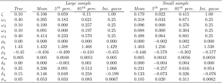
These results on identi…cation are of little practical use to us if the mechanism highlighted above does not work well in …nite samples. To analyze this issue we rely on a Monte Carlo exercise. We generate arti…cial data on aggregate nominal and real output using parameter values that roughly resemble what we …nd when we estimate the model with actual data. Then, we estimate the parameters of the model by maximum likelihood. We conduct both a large- and a small-sample exercise. Details and results are reported in the Appendix.
The bottom line is that, for large samples, the estimates are quite close to the true parameter values, and fall within a relatively narrow range. For samples of the same size as our actual sample, we also …nd the aggregate data to be informative of the distribution of sectoral weights. However, in this case the estimates are less precise and somewhat biased. This …nding underscores our case for incorporating prior information from the microeconomic evidence on price-setting, as we do in Section 4.3.
3
Empirical methodology and data
With the challenges involved in bridging the gap between price-setting statistics based on micro data and time series of aggregate nominal and real output, the choice of empirical methodology is critical. We employ a Bayesian approach, as this allows us to integrate those two sources of information.
With some abuse of notation, the Bayesian principle can be shortly stated as:
f( jZ ) =f(Z j )f( )=f(Z )/ L( jZ )f( );
wheref denotes density functions, Z is the vector of observed time series, is the vector of primitive parameters, andL( jZ ) is the likelihood function.
As observables, we use time series of aggregate nominal and real output. For constructing our prior distribution over the vector of sectoral weights,f(!1; :::; !K), we derive empirical distributions from Bils
and Klenow (2004) and Nakamura and Steinsson (2008), as discussed in detail in Subsection 3.1 below. In the next subsections we detail our prior distributions, sources of data, and estimation approach.
3.1 Prior over !
We specify priors over the set of sectoral weights ! = (!1; :::; !K), which are then combined with the
priors on the remaining parameters to produce the joint prior distribution for the set of all parameters of interest. We impose the combined restrictions of non-negativity and summation to unity of the
!’s through a Dirichlet distribution, which is a multivariate generalization of the beta distribution.
Notationally, ! D( 1; :::; K) with density function:
f!(!j 1; :::; K)/ K
Y
k=1
! k 1
k ; 8 k>0; 8!k 0; K
X
k=1
!k= 1:
The Dirichlet distribution is well known in Bayesian econometrics as the conjugate prior for the multino-mial distribution, and the hyperparameters 1; :::; K are most easily understood in this context, where
they can be interpreted as the “number of occurrences” for each of the K possible outcomes that the
econometrician assigns to the prior information.20 Thus, for given
1; :::; K, the parameter 0 Pk k
captures, in some sense, the overall level of information in the prior distribution. The information about the cross-sectional distribution of price stickiness comes from the relative sizes of the k’s. The latter
also determine the marginal distributions for the !k’s. For example, the expected value of!k is simply
20Gelman et al. (2003) o¤ers a good introduction to the use of Dirichlet distribution as a prior distribution for the
k= 0, whereas its mode equals( 0 K) 1( k 1)(provided that i>1 for all i).
Whenever we want to estimate a cross-sectional distribution of price rigidity based solely on aggregate data, we can impose an uninformative (“‡at”) prior, in which all ! vectors in the K-dimensional unit simplex are assigned equal prior density. This corresponds to k = 1 for all k – and thus 0 = K.
This allows us to extract the information that the aggregate data contain about the cross-sectional distribution of price stickiness.
To incorporate microeconomic information in the estimation, we relate the relative sizes of the hyperparameters ( 1; :::; K) to the empirical sectoral weights derived from the micro data, and choose
the value 0> K to determine the tightness of the prior distribution around the empirical distribution.
Speci…cally, let !b denote the set of sectoral weights from a given empirical distribution. We specify the relative sizes of the hyperparameters ( 1; :::; K) so that the mode of the prior distribution for !
coincides with the empirical sectoral weights!b. This requires setting k = 1 +!bk( 0 K). The case
of ‡at priors analyzed previously obtains when 0 =K. Henceforth, we refer to 0=K as the degree of
“prior informativeness”.
3.2 Priors on remaining parameters
The remaining parameters of the model fall into three categories that we deal with in turn. Our goal in specifying their prior distributions is to avoid imposing any meaningful penalties on most parameter values – except for those that really seem extreme on an a priori basis. The …rst set comprises the
’s and ’s, parameterizing the exogenous AR processes for nominal and natural output, respectively. These are assigned loose Gaussian priors with mean zero. We choose to …x the lag length at two for both processes, i.e. p1 = p2 = 2.21 The second set of parameters consists of the standard deviations
of the shocks to nominal ( m) and natural output ( n). These are strictly positive parameters to
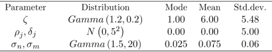
which we assign loose Gamma priors. The last parameter is the Ball-Romer index of real rigidity, , which should also be non-negative. This is captured with a very loose Gamma prior distribution, with mode at unity and a 5-95 percentile interval equal to (0:47;16:9). Hence, any meaningful degree of pricing complementarity or substitutability should be a result of the estimation rather than of our prior assumptions. These priors are summarized in Table 1.22
21In principle we could specify priors over p
1; p2 and estimate their posterior distributions as well. However, the
computational cost of estimating all the models in the paper is already quite high, and we restrict ourselves to this speci…cation with …xed number of lags. Our conclusions are robust to alternative assumptions about the number of lags (see Section 5).
22We do not include in the estimation, and set = 0
Table 1: Prior distributions for remaining parameters
Parameter Distribution Mode Mean Std.dev.
Gamma(1:2;0:2) 1:00 6:00 5:48
j; j N 0;52 0:00 0:00 5:00 n; m Gamma(1:5;20) 0:025 0:075 0:06
Note: The hyper-parameters for the Gamma distribution specify shape and inverse scale, respectively, as in Gelman et al. (2003).
3.3 Macroeconomic time series
We estimate the model using quarterly data on nominal and real output for the U.S. economy. These are measured as seasonally-adjusted GDP at, respectively, current and constant prices, from the Bureau of Economic Analysis. We take natural logarithms and remove a linear trend from the data. Whereas the assumptions underlying the model include one of an unchanged economic environment, the U.S. economy has undergone profound changes in the recent decades, including the so-called “Great Moderation” and the Volcker Disin‡ation. As a consequence, we choose not to confront the model with the full sample of post-war data. We use the period from 1979 to 1982 as a pre-sample, and evaluate the model according to its ability to match business cycle developments in nominal and real output in the period 1983-2007.23
3.4 Empirical distributions of price stickiness
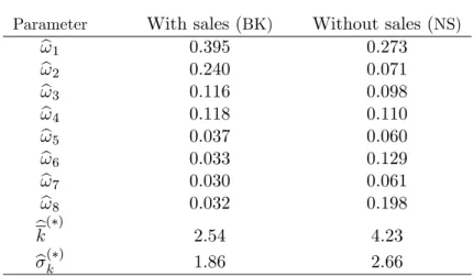
We work with the statistics on the frequency of price changes for the 350 categories of goods and services (“entry level items”) reported by Bils and Klenow (2004, henceforth BK), and with the 272 entry level items covered by Nakamura and Steinsson (2008, henceforth NS). In the latter case we use the statistics for regular prices (those excluding sales and product substitutions). We refer to the corresponding empirical distributions of price rigidity as distributionswith (BK) andwithout (NS) sales.
Our goal is to map those statistics into an empirical distribution of sectoral weights over spells of price rigidity with di¤erent durations. We work at a quarterly frequency, and for computational reasons consider economies with at most 8 quarters of price stickiness. Sectors correspond to price spells which are multiples of one quarter. We denote an empirical cross-sectional distribution of price rigidity by
f!bkg8k=1, whereb!1 denotes the fraction of …rms that change prices every quarter,b!2 the fraction with an
expected duration of price spells between one (exclusive) and two quarters (inclusive), and so on. The sectoral weights are aggregated accordingly by adding up the corresponding CPI expenditure weights. We proceed in this fashion until the sector with 7-quarter price spells. Finally, we aggregate all the
23We make use of the pre-sample 1979-1982 by initializing the Kalman …lter in the estimation stage with the estimate of
remaining categories, which have mean durations of price rigidity of8quarters and beyond, into a sector with2-year price spells. This gives rise to the empirical cross-sectional distributions of price stickiness that we use in our estimation, which are summarized in Table 2. We denote the sectoral weight for sectorkobtained from this procedure byb!k. For each of the BK and NS distributions, we also compute
the average duration of price spells, bk = P8k=1!bkk; and the cross-sectional standard deviation of the
underlying distribution,bk=
r P8
k=1b!k k bk
2
.
Table 2: Empirical cross-sectional distributions of price stickiness
Parameter With sales (BK) Without sales (NS)
b
!1 0:395 0:273
b
!2 0:240 0:071
b
!3 0:116 0:098
b
!4 0:118 0:110
b
!5 0:037 0:060
b
!6 0:033 0:129
b
!7 0:030 0:061
b
!8 0:032 0:198
b
k( ) 2:54 4:23
b( )k 1:86 2:66
(*) In quarters. P!bkmight di¤er from unity due to rounding.
3.5 Simulating the posterior distribution
The joint posterior distribution of the model parameters is obtained through application of a Markov-chain Monte Carlo (MCMC) Metropolis algorithm. The algorithm produces a simulation sample of the parameters that converges to the joint posterior distribution under certain conditions.24 We provide
details of our speci…c estimation process in the Appendix. The outcome is a sample of one million draws from the joint posterior distribution of the parameters of interest, based on which we draw the conclusions that we start to report in the next section.
Having obtained a sample of the posterior distribution of parameters from any given model, we can estimate the marginal posterior density (henceforthmpd) of the data given the model as:
mpdj =f(Z jMj) =
Z
L( jZ ;Mj)f( jMj)d ; (14)
and use it for model-comparison purposes. In (14), Mj refers to a speci…c con…guration of the model
and prior distribution, and f( jMj) denotes the corresponding joint prior distribution. Speci…cally,
we approximate log(mpdj) for each model using Geweke’s (1999) modi…ed harmonic mean. We use
these estimates to evaluate the empirical …t of the models relative to one another. The mpd ratio of
two model con…gurations constitutes the Bayes factor, and – when neither con…guration is a priori
considered more likely – theposterior odds. It indicates how likely the two models are relative to one
another given the observed dataZ .
4
Results
4.1 Macro-based estimates
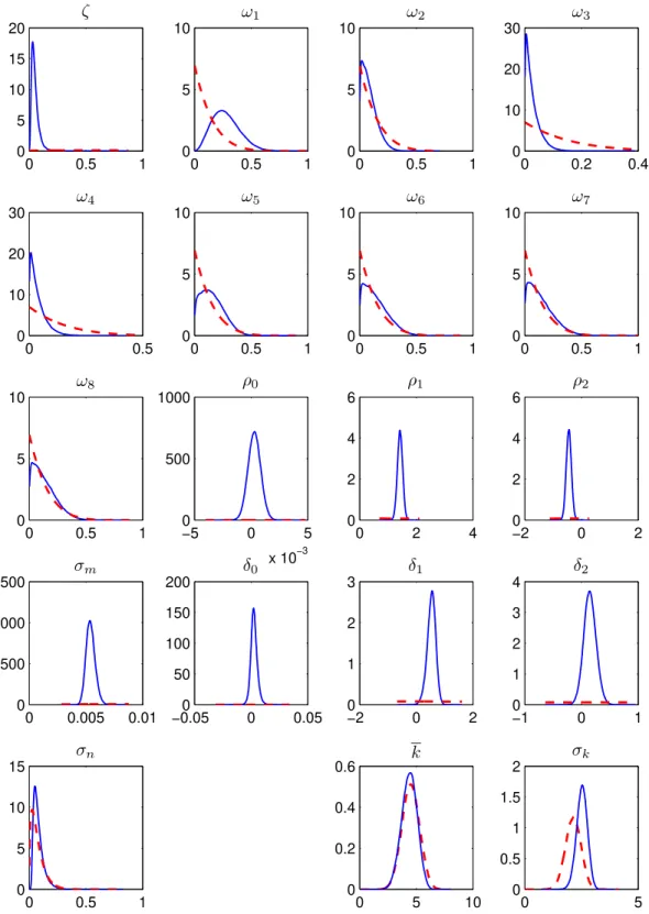
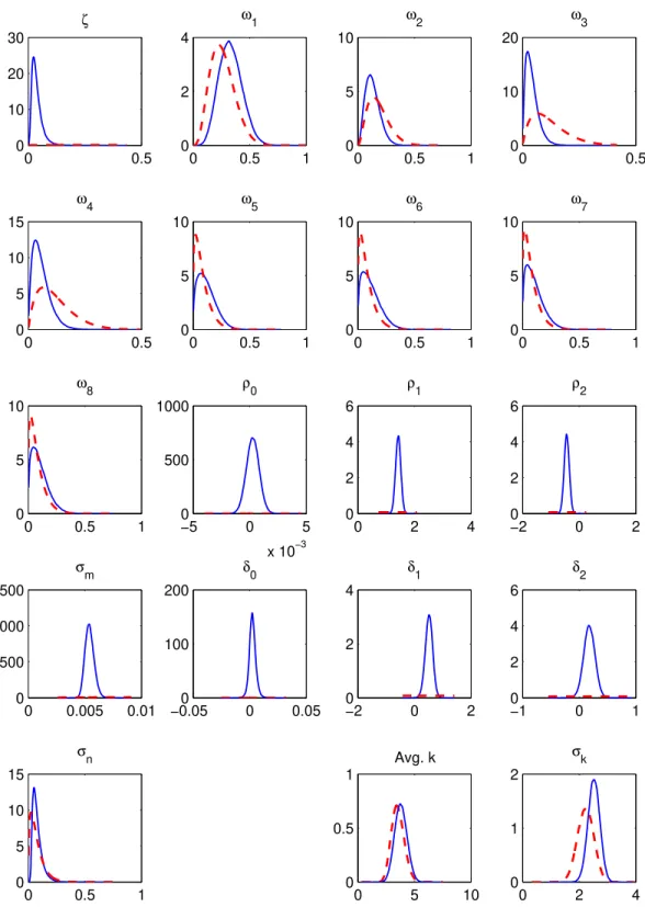
Table 3 and Figure 1 report the results for the case of uninformative priors, in terms of marginal distri-butions for the parameters.25 The empirical distributions of price rigidity from Table 2 are reproduced
in the last columns, for ease of comparison. In what follows, we use the posterior means as the point estimates for the sectoral weights, reported in the third column of the table.26
The cross-sectional distributions that we infer from aggregate data conform quite well with the empirical ones. The macro-based estimates imply that approximately 28% of …rms change prices every quarter; 43% change prices at least once a year; 13% change prices once every two years. The average duration of price spells is 13 months, and the standard deviation of the duration of price spells is approximately 8 months. These numbers are quite close to the empirical distribution without sales and product substitutions (last column of the table). The correlation between our macro-based estimates and those empirical weights is 0:63. The correlation of the estimates with the empirical distribution with sales and product substitutions is somewhat lower, at0:43. This is a …rst, informal indication that the distribution that excludes sales and product substitutions helps the model …t aggregate dynamics better. Below we investigate this possibility by performing formal model comparisons using a standard measure of …t.
The index of real rigidities implies strong pricing complementarities. The posterior mean of is 0.05 and the 95th percentile equals 0.11, which falls within the 0.10-0.15 range that Woodford (2003)
argues can be made consistent with fully speci…ed models. As highlighted by Carvalho (2006), such complementarities interact with heterogeneity in price stickiness to amplify the aggregate e¤ects of nominal rigidities in this type of sticky-price model.
25We use a Gaussian kernel density estimator to graph the marginal posterior density for each parameter. The priors
onkand k are based on 100,000 draws from the prior Dirichlet distribution.
26The results are almost insensitive to using alternative point estimates, such as the values at the joint posterior mode,
Table 3: Parameter estimates under a ‡at prior
k = 1f or all k ( 0= 8) Empirical distributions
W ith sales W=o sales
4:440
(0:466;16:863) (0:015;00:042:111) 0:050
!1 0:094
(0:007;0:348) (0:099;00:264:493) 0:276 0:395 0:273
!2 0:094
(0:007;0:348) (0:007;00:072:212) 0:086 0:240 0:071
!3 0:094
(0:007;0:348) (0:002;00:020:078) 0:027 0:116 0:098
!4 0:094
(0:007;0:348) (0:002;00:027:107) 0:037 0:118 0:110
!5 0:094
(0:007;0:348) (0:017;00:144:337) 0:156 0:037 0:059
!6 0:094
(0:007;0:348) (0:011;00:123:345) 0:144 0:033 0:129
!7 0:094
(0:007;0:348) (0:010;00:120:353) 0:143 0:030 0:061
!8 0:094
(0:007;0:348) (0:010;00:112:323) 0:132 0:032 0:198
k 4:501
(3:245;5:760) (3:214;54:394:462) 4:37 2:54 4:25
k 2:139
(1:584;2:678) (2:112;22:523:893) 2:62 1:86 2:66
0 0:000
( 8:224;8:224) ( 0:0001;0:000:001) 0:000
1 0:000
( 8:224;8:224) (1:273;11:426:576) 1:426
2 0:000
( 8:224;8:224) ( 0:593; 00:446:296) 0:446 m 0:059
(0:009;0:195) (0:005;00:005:006) 0:005
0 0:000
( 8:224;8:224) ( 0:0002;0:002:007) 0:003
1 0:000
( 8:224;8:224) (0:270;00:541:763) 0:532
2 0:000
( 8:224;8:224) ( 0:0027;0:146:331) 0:149 n 0:059
(0:009;0:195) (0:030;00:069:172) 0:081
Note: The …rst two columns report the medians of, respectively, the marginal prior and posterior distributions; the third column gives the mean of the marginal posterior distribution; numbers in parentheses correspond to the 5th and 95th percentiles; the
4.2 Comparison with homogeneous-…rms models
In this subsection we ask how sharply the data allow us to discriminate between multi-sector models with heterogeneity in price stickiness and one-sector models with homogeneous …rms. To that end, we estimate one-sector models with price spells ranging from two to eight quarters. We keep the same prior distributions for all parameters besides the sectoral weights. A one-sector model with price spells of lengthk, say, can be seen as a restriction of the multi-sector model, with a degenerate distribution of sectoral weights (!k= 1,!k0 = 0 for allk0 6=k).
We pick the best-…tting one-sector model according to the marginal density of the data given the models. The results are reported in Table 4 and Figure 2. The best-…tting model is the one in which all price spells last for 7 quarters. This seems unreasonable in light of the microeconomic evidence. Given the extent of nominal rigidity, not surprisingly the degree of pricing complementarity is smaller. The posterior distributions for the parameters of the nominal output process are quite similar to the ones obtained in the multi-sector models. Perhaps this should be expected given that this variable is one of the observables used in the estimation. In contrast, the distributions of the parameters of the unobserved driving process are di¤erent under the restriction of homogeneous …rms. We defer a discussion of what might drive this result to the end of this subsection.
Table 4: Best-…tting homogeneous economy
Prior K= 7,!7= 1
4:440
(0:466;16:863) (0:193;00:362:830) 0:419 0 ( 80:000
:224;8:224) ( 0:0001;0:000:001) 0:000 1 ( 80:000
:224;8:224) (1:284;11:430:568) 1:428 2 0:000
( 8:224;8:224) ( 0:590; 00:454:310)
0:452
m 0:059
(0:009;0:195) (0:005;00:005:006) 0:005 0 0:000
( 8:224;8:224) ( 0:0003;0:003:011) 0:004 1 0:000
( 8:224;8:224) ( 0:0154;0:064:319) 0:071 2 0:000
( 8:224;8:224) ( 0:0027;0:135:327) 0:141
n 0:059
(0:009;0:195) (0:087;00:216:421) 0:230
Note: The …rst two columns report the medians of, respectively, the marginal prior and posterior distri-butions; the third column gives the mean of the mar-ginal posterior distribution; numbers in parentheses correspond to the 5th and 95th percentiles.
the multi-sector model has more parameters than the homogeneous-…rms model.27
Table 5 reports the results for the multi-sector model with the ‡at prior for !, and the best-…tting one-sector model. The …t of the multi-sector model is much better than that of the best-…tting one-sector model: the posterior odds in favor of the former model is of the order of1011: 1.
Table 5: Model comparison - heterogeneous versus homogeneous economy
Multi-sector model
Best-…tting 1-sector model logmpd 808:03 781:33
Note: The logarithm of the marginal posterior den-sity of the data given the models (log mpd) is
ap-proximated with Geweke’s (1999) modi…ed harmonic mean.
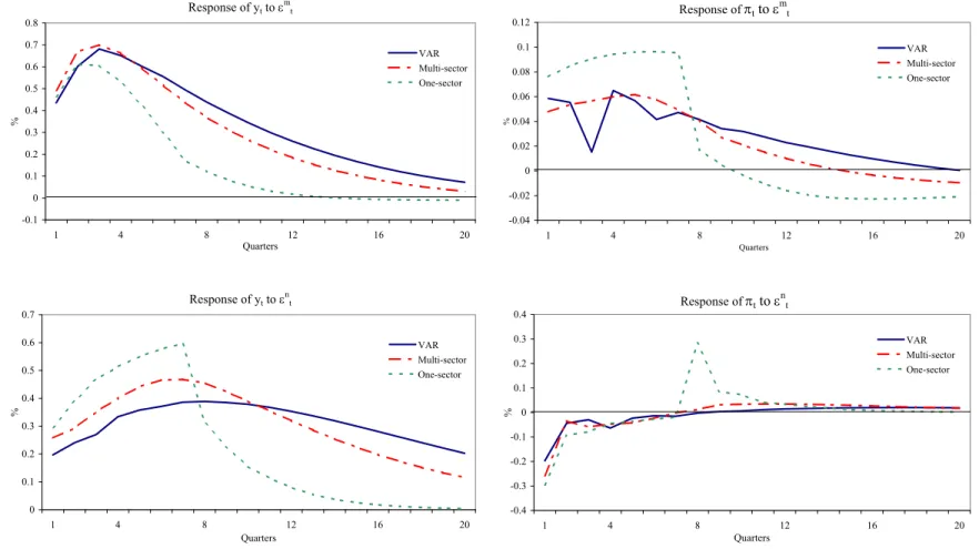
Our model-comparison criterion has the disadvantage that it does not provide any information on what drives the improved empirical …t of the multi-sector model. To shed some light on this question we compare model-implied dynamics for in‡ation and output to those of a restricted bivariate VAR including nominal and real output. In estimating the VAR we impose the same assumption used in the models, that nominal output is exogenous and follows an AR(2) process. We allow real output to depend on four lags of both itself and nominal output, and to be contemporaneously a¤ected by innovations to nominal output. Estimation is by ordinary least squares. The multi-sector model is the one estimated under ‡at priors for !, while the one-sector model is the one with the best …t. The parameter values are …xed at their posterior means. Since the impulse response functions are conditional on speci…c parameter values, the comparison does not correct for the larger number of parameters in the multi-sector model. Thus, it is only meant to provide some indication of the sources of the large di¤erences in the posterior odds of the models.
The panel in Figure 3 shows the impulse response functions of output (yt, left column) and in‡ation
( t, right column) to positive innovations"mt (top row) and"nt (bottom row) of one standard deviation
in size.28 Relative to the one-sector model, the estimated multi-sector model does a better job at
approximating the impulse response functions produced by the VAR at both short and medium horizons, in response to both shocks. Thus the overwhelming statistical support for heterogeneity does not seem to depend on any single feature of the dynamic response of macroeconomic variables to the shocks. Finally, these results suggest one explanation for why the estimated parameters associated with the unobserved driving process are di¤erent in the one-sector economy. While the multi-sector model can rely on the distribution of sectoral weights to balance the response of the economy to shocks at di¤erent
27The reason is that the vector of parameters is “integrated out” in (14). 28Following the notation of the semi-structural model, in the VAR"m
horizons, the one-sector model lacks this mechanism. Given the facts that nominal output is observed and that its parameter estimates imply quite persistent dynamics in both economies, perhaps the one-sector economy needs to rely on the unobserved process as a more transient and volatile component that can help it do a better job at matching higher-frequency features of the data.
4.3 Combining micro and macro data in the estimation
We now turn to estimations that incorporate information from price-setting statistics derived from micro data. Table 6 and Figures 4-7 present the results for two sets of informative priors ( 0=K = 2;
5) for each empirical distribution. The bottom row of Table 6 reports the log of the posterior marginal
density of the various models. For the less informative set of priors ( 0=K = 2) the two empirical
distributions that inform the prior lead to models that perform similarly in terms of …t – and close to the model estimated under a ‡at prior. However, for the more informative set of priors ( 0=K = 5),
the model with prior based on the empirical distribution of price rigidity without sales …ts the data better according to the posterior marginal density criterion – the di¤erence of4:4 log-points implies a posterior odds ratio of roughly80 : 1 in favor of the model with prior distribution that excludes sales
and product substitutions.
We can use such a comparison of posterior marginal densities of various estimated models for assess-ing the relative merits of the two sets of priors for the purpose of helpassess-ing the model explain aggregate dynamics. To that end, we estimate a series of additional models with informative priors based on the two empirical distributions of price rigidity (with and without sales), progressively increasing the degree of prior informativeness (i.e., increasing 0=K). Speci…cally, we estimate additional models
with 0=K = 10;20;100, and1000. In addition, we estimate models in which the distribution of price
stickiness that forms the prior has equal weights in all sectors (“uniform prior”). We summarize the results in Figure 8. It shows clearly that the di¤erence between the …t of estimated models increases as the priors become more informative. While the di¤erence in …t between the models based on the prior distribution without sales and the uniform prior is not that large (it tends to approximately 3 log-points for very informative priors), the di¤erence between models based on prior distributions with and without sales is more substantial. As the degree of prior informativeness increases, that di¤erence approaches 6 log-points – which translates into a posterior odds ratio of roughly 400 : 1in favor of the model with prior distribution that excludes sales and product substitutions.29
29Figure 8 also shows that, as we tighten the priors on the sectoral weights, the …t of models estimated under priors
Table 6: Parameter estimates with informative priors
Inf orm: prior, 0=K= 2 Inf orm: prior, 0=K = 5 F lat prior Empirical distributions
W ith sales W=o sales W ith sales W=o sales W ith sales W=o sales
0:032
(0:01;0:08) (00:02;0:042:11) (00:01;0:018:05) (0:002;0:041:10) (00:02;0:042:11)
!1 0:324
(0:17;0:51) (00:14;0:277:45) (00:31;0:425:55) (0:021;0:309:43) (0:0099;0:264:49) 0:395 0:273
!2 0:123
(0:04;0:24) (00:01;0:069:18) (00:11;0:190:29) (0:002;0:059:13) (0:001;0:072:212) 0:240 0:071
!3 0:035
(0:01;0:09) (00:01;0:033:09) (00:02;0:059:11) (0:002;0:051:10) (0:000;0:020:08) 0:116 0:098
!4 0:049
(0:01;0:13) (00:01;0:047:12) (00:03;0:081:15) (0:003;0:072:14) (0:000;0:027:11) 0:118 0:110
!5 0:106
(0:02;0:26) (00:02;0:109:26) (00:01;0:056:15) (0:002;0:066:15) (0:001;0:144:34) 0:037 0:059
!6 0:100
(0:01;0:27) (00:04;0:142:31) (00:01;0:052:15) (0:007;0:144:25) (0:001;0:123:35) 0:033 0:129
!7 0:090
(0:01;0:25) (00:01;0:086:24) (00:00;0:042:13) (0:002;0:058:14) (0:001;0:120:35) 0:030 0:061
!8 0:088
(0:01;0:24) (00:05;0:160:32) (00:01;0:044:13) (0:011;0:200:31) (0:001;0:112:32) 0:032 0:198
k 3:776
(2:91;4:69) (34:45;5:367:25) (22:31;3:811:40) (3:460;4:262:91) (3:421;5:394:46) 2:54 4:25
k 2:515
(2:17;2:85) (22:28;2:612:91) (12:81;2:184:56) (2:250;2:725:93) (2:211;2:523:89) 1:86 2:66
0 0:000
( 0:00;0:00) ( 00::00;0000:00) ( 00:00;0:000:00) ( 00::00;0000:00) ( 00::00;0000:00)
1 1:425
(1:27;1:57) (11:27;1:427:58) (11:27;1:424:57) (1:128;1:429:58) (11:27;1:426:58)
2 0:445
( 0:59; 0:30) ( 0:59; 00:447:30) ( 0:59; 00:444:29) ( 0:60; 00:449:30) ( 0:59; 00:446:30) m 0:005
(0:00;0:01) (00:00;0:005:01) (00:00;0:005:01) (0:000;0:005:01) (00:00;0:005:01)
0 0:002
( 0:00;0:01) ( 00::00;0002:01) ( 00:00;0:002:01) ( 00::00;0002:01) ( 00::00;0002:01)
1 0:514
(0:30;0:72) (00:32;0:545:75) (00:28;0:465:65) (0:038;0:563:75) (00:27;0:541:76)
2 0:176
(0:01;0:34) ( 00::01;0151:32) (00:06;0:201:34) ( 00::01;0146:30) ( 00::03;0146:33) n 0:068
(0:03;0:16) (00:03;0:066:16) (00:03;0:072:17) (0:003;0:062:15) (00:03;0:069:17)
logmpd 807:56 808:27 803:768 808:16 808:03
5
Robustness
Our …ndings are robust to di¤erent prior assumptions for the parameters i, i, m, nand , as well as
di¤erent de-trending procedures and speci…cations for the exogenous time-series processes. In particular, they are robust to using a Baxter and King (1999) …lter or …rst-di¤erences instead of removing linear trends from the data, and to assuming AR(3) exogenous processes (i.e.,p1 =p2 = 3). Also, unreported
results with models with K < 8 suggest that one needs to allow for “enough” heterogeneity in order
to avoid compromising the empirical performance of the model. In particular, the …t of models with
K= 4 (as in Coenen et al. 2007) is much worse than models with K= 6 or8. While the di¤erences in
empirical performance between models withK = 6and K = 8 are not that large, the evidence against the speci…cations with K = 4 is quite strong: posterior odds ratios favor the models with K = 6;8 by
an order of105 : 1.
In the sections below we discuss the robustness of our …ndings to alternative models of price setting. In particular, we consider the Calvo (1983) model, and discuss a new model of price setting that produces the exact same results as our model, and yet can speak to a much larger set of empirical facts about price setting derived from micro data.
5.1 Results under the Calvo (1983) model
We also considered versions of the model with Calvo (1983) pricing. Mimicking our baseline analysis, the …rst step is to show that the model allows for identi…cation of the cross-sectional distribution of price rigidity from aggregate data, and, given that result, that it also allows for separate identi…cation of nominal and real rigidities. Indeed, all identi…cation results go through, and the intuition is very similar to the one in the Taylor model. In the Appendix we provide a thorough proof of identi…cation, including the case with strategic interactions in price-setting decisions (i.e., index of real rigidities 6= 1).
However, under Calvo pricing, not all of our conclusions are equally robust when it comes to relatively small samples. The reason is that, in the context of our semi-structural framework, identi…cation of heterogeneity in price stickiness under Calvo pricing is “more di¢cult” than under Taylor pricing. Building on Monte Carlo analysis and analytical insights from simple versions of these two pricing models, we found that clear-cut identi…cation of the distribution of price stickiness depends on whether the observable driving process has high variance relative to the unobservable process.
criterion fails to provide a sharp discrimination between alternative (non-degenerate) distributions of price stickiness under Calvo pricing. This mirrors what we …nd in the data: under Calvo pricing, they do not allow too sharp a discrimination between di¤erent models with heterogeneity in price stickiness. In contrast, given the same sample size and relative variances for those two processes, the version of the model with Taylor pricing provides more information about the underlying distribution of price stickiness – as seen in previous sections.
However, despite that di¢culty, our main …ndings do hold under the Calvo pricing model – at least qualitatively. First, on the comparison between models with heterogeneity in price stickiness and models with homogeneous …rms, the estimated models provide clear evidence in favor of the former. Speci…cally, we …nd that a likelihood-ratio test of the homogeneous Calvo model against multi-sector versions of the model leads to rejection of the former at signi…cance levels of less than 1%.30 Second,
all estimated models feature < 1, implying strategic complementarities in price setting. Finally, estimations under informative priors derived from the empirical distributions of price stickiness (as described in Section 3) also provide (qualitative) evidence in favor of the distribution that excludes sales and product substitutions.31
5.2 An alternative model
As we mentioned in Section 2, the Taylor model is, strictly speaking, at odds with the microeconomic evidence on the duration of price spells (e.g., Klenow and Kryvtsov 2008). This inconsistency may be viewed as a weakness of the Taylor model relative to alternatives – in particular the Calvo model, which naturally produces a non-degenerate distribution of the duration of price spells at the …rm level.
However, this evidence does not invalidate the use of that model for our purposes. To show that this is the case, here we provide an alternative model in which the duration of price spells varies at the …rm level. The model can match the empirical distribution of the duration of price spells. Yet, the aggregate behavior of the model is identical to the one presented in Section 2. Furthermore, this alternative model can match additional micro facts documented in the literature – in a similar fashion as the Calvo (1983) model.
There is a continuum of monopolistically competitive …rms divided into N “economic” sectors (i.e.,
30Real and nominal rigidities are not separately identi…ed in our Calvo model with homogeneous price stickiness. As
a result, comparisons based on the log posterior marginal density are sensitive to the prior on the index of real rigidities (even though we use a very uninformative prior). Hence, in this case we …nd it more appropriate to use a criterion based only on the likelihood.
31That is, the log posterior density of the data given the model is always higher under informative priors based on the
not necessarily identi…ed by price stickiness). Sectors are indexed byn2 f1; :::; Ng. The distribution of …rms across sectors is summarized by a vector ('1; :::; 'N) with'n>0;PNn=1'n= 1, where 'n gives the mass of …rms in sectorn. Each sector has a (sector-speci…c) stationary cross-sectional distribution of price stickiness. Before setting its price, a …rmjin economic sector nmakes a draw for the duration of its next price spell, and then sets its price optimally. Notice that the price will be chosen according to the same policy as in the Taylor model (i.e., the optimal price for a spell that will last for a known duration). This implies that, at a given time, …rms within a given sector can be further divided into di¤erent “groups” depending on the duration of price spells that they draw.
The (also stationary) cross-sectional distribution of price stickiness for the entire economy can be constructed by aggregating across sectors. It is summarized by a vector (!1; :::; !K) with !k
PN
n=1'n!n;k 2(0;1). It is easy to show thatPKk=1!k = 1:
XK
k=1
XN
n=1'n!n;k=
XN
n=1
XK
k=1'n!n;k=
XN
n=1'n
XK
k=1!n;k = 1:
The exact details of how each …rm draws the duration for the new price spell – that is, how …rms move around di¤erent “stickiness groups” within a sector – is inconsequential for the aggregate dynamics implied by this model. What matters is our assumption that the cross-sectional distribution of price stickiness of each sector is stationary (i.e. !n;k is time-invariant), which guarantees the stationarity
of the economy-wide distribution of price stickiness. In the Appendix we provide an example with a ‡exible scheme for drawing durations within each sector, which allows for persistence in the duration of price spells at the …rm level.
We can write the log-linear approximate model implied by this “Random Taylor” price-setting scheme as:
xt(k) =
1
1 kEt
k 1
X
i=0
i p
t+i+ yt+i ytn+i ;
pt = N
X
n=1
'npt(n);
pt(n) = K
X
k=1
!n;kpt(n; k);
pt(n; k) =
Z 1
0
pt(n; k; j)dj =
1 k
k 1
X
j=0