Do market indices overreact?

(1)

M

ASTER OF

S

CIENCE IN

FINANCE

M

ASTER

´

S

F

INAL

W

ORK

D

ISSERTATION

DO MARKET INDICES OVERREACT

?

LUÍS FILIPE CORDEIRO CARVALHO

(2)

MASTER OF SCIENCE IN

FINANCE

M

ASTER

´

S

F

INAL

W

ORK

D

ISSERTATION

DO MARKET INDICES OVERREACT

?

LUÍS FILIPE CORDEIRO CARVALHO

S

UPERVISION

:

PROFESSOR DOUTOR JOÃO LUÍS CORREIA DUQUE

PROFESSOR DOUTOR PAULO FERNANDO DE SOUSA PEREIRA ALVES

(3)

Resumo

Entende-se por sobreajustamento de mercado quando o optimismo (pessimismo) por parte dos investidores leva a que o preço da ação de uma empresa suba (desça) de tal forma que esta é considerada vencedora (perdedora), num período compreendido de 3 a 5 anos. Esta dissertação estuda a hipótese de sobreajustamento nos índices de mercado. Utilizando dados mensais de dezembro 1970 a dezembro 2018 de 49 índices internacionais da Morgan Stanley Capital, foi estudada a hipótese de sobreajustamento nos índices de Mercado para períodos de 3 e 5 anos. Ao invés de retornos cumulativos os retornos foram calculados segundo a metodologia de investimento passivo com o intuito de evitar enviesamentos. Foram encontradas fortes reversões dos retornos para períodos de investimento de 3 anos, e estatisticamente significativos. Quando implementada a estratégia de comprar os maiores perdedores e vender os maiores vencedores apenas em índices de mercados desenvolvidos, encontra-se igualmente evidência para a hipótese de sobreajustamento, ainda que os retornos sejam menos expressivos do ponto de vista económico. Foi igualmente encontrada evidência para a hipótese de sobreajustamento quando se considera períodos de investimento de 5 anos, com resultados estatisticamente significativos. Os perdedores não só têm rendibilidades superiores aos ganhadores, como apresentam menos risco. Independentemente do período de investimento, anos da amostra ou do tipo de mercado o Beta do portfólio de perdedores foi, em média, inferior ao do portfólio de vencedores. Não obstante estes resultados, a hipótese de sobreajustamento aparenta não ser estacionária no tempo.

Palavras-Chave: índices de Mercado, sobreajustamento de mercado, reversão de retornos Códigos: G10, G14, G15, G40

(4)

Abstract

Investors are told to be overreacting when their sentiment drives the price of a certain security up (down) enough to make it the biggest winner (loser), in most cases considering this overreaction period as long as 3 or 5 years. This dissertation studies the overreaction hypothesis in market indices. Using end of month data from December 1970 to December 2018 from 49 Morgan Stanley Capital International Indices we studied the overreaction hypothesis on Market Indices for 3- and 5-years’ investment periods. Instead of Cumulative Average Returns the returns were computed as Holding Period Returns to avoid the upward bias. We found strong return reversals for 3-year investment periods, which were statistically significant at a 5% significant level. However, the returns might be weaker depending on the time period we consider. When implemented only in developed markets there is still evidence supporting the overreaction hypothesis, although the excess returns are economically weaker. Evidence for the overreaction hypothesis was also found when 5-year investment periods were considered. Not only did losers outperform winners, but they were also less risky than winners. Regardless of the market, investment period and/or time-period considered, losers’ portfolio beta was always smaller than the winners’ portfolio beta. Notwithstanding these results, the overreaction strategy is sensitive to the time periods considered which highlights the possibility that the overreaction strategy success it’s not time stationary.

Keywords: Market indices, overreaction hypothesis, winner-losers’ reversals JEL Codes: G10, G14, G15, G40

(5)

Acknowledgements

This thesis means the end of a 5-year journey at ISEG. Looking back in time I couldn’t be happier with the choice I made in 2014, and especially with my decision in 2017 to enroll in the master in finance at ISEG. This journey allowed me not only to learn about economics and afterwards about finance but was also a chance to meet highly intelligent and tremendous well-intentioned people, which today I have the pleasure to call friends. Albeit filled with good memories that I will cherish in the future; this journey was also highly demanding. The last year was the year where I felt most challenged and went beyond what I thought were my limits. Having decided to do an internship at CMVM1

while finishing my masters’ degree was probably one the best, but also one of the toughest decisions I ever made. Striving for excellence during my master, while coupling with the daily work at CMVM, an organization that is changing and always settles for the highest standards, made me the professional, but above all the person I am today. This journey couldn’t have been possible without the support of the ones who have always stood beside me. First and foremost, I would like to thank my supervisors Professor Doutor João Luís Correia Duque and Professor Doutor Paulo Fernando de Sousa Pereira Alves. The time both of them dedicated to help me in this writing procedure, their insights and guidance proved to be highly valuable, and profoundly necessary to the development of this work. To both of them my sincere thank you. I would also like to express my gratitude towards CMVM’s Ongoing Supervision Department. My experience and lessons learned during my internship at CMVM helped me during this procedure, which couldn’t have been possible without the persons with whom I worked with. To my friends. While the last year has been more time-consuming for me, it wouldn’t have been the same without their companionship and cheerful moments. Last, but not the least, I am forever thankful to my Family, especially to my Parents. Their unconditional love and support allowed me to pursue my ambitions, to never give up of my goals and always shoot for the stars. Part of who I am I owe it to them.

(6)

List of Abbreviations AR – Abnormal Returns

BH – Buy-and-Hold

CAPM – Capital Asset Pricing Model CAR – Cumulative Average Return EMH – Efficient Market Hypothesis ER – Excess Returns

EMR – Excess Market Return HPR - Holding Period Return

MSCI – Morgan Stanley Capital International

PRIIPs - Packaged Retail Investment and Insurance-Based Products UK- United Kingdom

US – United States

(7)

Contents Resumo ... i Abstract ... ii Acknowledgements ... iii List of Abbreviations ... iv List of Tables ... vi List of Figures ... vi Introduction ... 1 1. Literature Review ... 3

2. Data and methodology ... 7

2.1. Methodology for Excess Returns ... 9

2.2. Methodology for Risk-Adjusted Returns ... 11

3. Excess Returns ... 12 3.1. 3-year periods ... 12 3.2. 5-year periods ... 18 4. Risk-adjusted Returns ... 20 4.1. 3-year periods ... 20 4.2. 5-year periods ... 24 Conclusions ... 27

Limitations and further research ... 28

(8)

List of Tables

Table I. MSCI Indices Annual Returns ... 8

Table II. Contrarian Strategy success ... 12

Table III. Excess Returns (3-y Ranking) ... 14

Table IV. Excess Returns in Developed Markets (3-y ranking) ... 15

Table V. Excess Returns by Market (3-y ranking) ... 17

Table VI. Excess Returns (5-y ranking) ... 18

Table VII. Excess Returns in Developed Markets (5-y ranking) ... 19

Table VIII. Risk-Adjusted Returns (3-y ranking) ... 20

Table IX. Risk-Adjusted Returns in developed markets (3-y ranking) ... 22

Table X. Risk-Adjusted Returns by Market (3-y ranking) ... 23

Table XI. Risk-Adjusted Returns (5-y ranking) ... 25

Table XII. Risk-Adjusted Returns in developed markets (5-y ranking) ... 25

List of Figures Figure 1. Growth of hypothetical $10,000 by market ... 9

(9)

Introduction

“We have far too many ways to interpret past events for our own good”, Nassim Nicholas Taleb

Whether is routine, when someone wants to purchase a new device, to book a restaurant, to buy a new car there is a high chance that people will rely in the past and/or their past experiences to decide. The world of finance is no exception to this matter. It is not unusual to see people deciding how to invest their money based on the historical performance of financial securities and see them pick what they think is a “good” investment. In fact, Commission Delegated Regulation (EU) 2017/653 requires that Packaged Retail Investment and Insurance-Based Products’ (PRIIPs) Key Investor Information document have the following disclaimer: “The scenarios presented are an estimate of future

performance based on evidence from the past on how the value of this investment varies, and are not an exact indicator. What you get will vary depending on how the market performs and how long you keep the investment/product”. Such practice shows how the

past is deeply rooted in people’s decisions and mindset, but also how the financial sector still relies on historical data. Using historical data in our decision-making processes, especially in finance might be a usual thing to do but was believed to be useless as Eugene Fama pointed out. According to the Efficient Market Hypothesis (EMH), prices reflect all available information in the market and any form of abnormal returns, alpha, was deemed as impossible. Comprised by three forms of efficiency, the weak form, semi-strong and semi-strong form, the weakest form held that future prices could not be predicted by analyzing historical prices, and any form of abnormal returns could not be achieved with investment strategies built upon historical data. De Bondt and Thaler (1985) studied the EMH in the US Equity Markets and found unpredictable results. Not only did losers, securities with extreme negative past returns, outperformed winners, securities with extreme positive past returns, but according to the Capital Asset Pricing Model (CAPM) the former were also less risky. If the weakest form of the EMH holds, it is impossible for an investor to create profitable investment strategies using historical data. The only way for an investor to get higher returns is through an higher risk exposure. De Bondt and Thaler (1985) seemed to have found not only an investment strategy that would yield

(10)

excess returns using historical data, but also that contradicted the EMH previously discussed in Fama and MacBeth (1973). The reason for such returns was said to be Market overreaction. As explained more exhaustively in Thaler, R.H. (2015), by ranking firms’ stocks based on their past 3 to 5 years returns the authors provided enough time for investors to formulate their expectations regarding a certain company and become too optimistic or pessimistic about that company. Assuming that this optimistic (pessimist) mindset drove the price of a certain stock up (down) enough to make it the biggest winner (loser) over a period of 3 to 5 years, investors were expected to be overreacting to something. Albeit exhaustively studied in Equity Markets, especially the US Equity Markets, the phenomenon of overreaction applied to Market Indices still lacks some proper answers. Richards (1997) used data from 16 Country Indices and found evidence for return reversals. More surprisingly, risk was not an explanation for this phenomenon, given the fact that loser indices were not riskier than winner indices. While the study had some limitations namely the number of countries included in the sample, it was important to spark the debate about national stock market indices overreaction. Therefore, this work intends to find a proper answer to the following question “Do Market Indices overreact?”. For such it will be used end of month data from December 1970 to December 2018 from 49 Morgan Stanley Capital International Indices. The Total Returns Country Indices will be used which include the reinvested gross dividends in US dollars. The software used was the 14.1 version of Stata. In the 1st_{chapter it will be presented a literature review}

about the topic of return reversals, especially the 1st_{findings for return reversals in the}

US market followed by further research on market overreaction for other markets and country indices. In the 2nd_{chapter we present the Data and methodology to study our}

hypothesis. Both excess returns and risk-adjusted returns were used in order to test the hypothesis. While the 1st_{allow us to see how the indices compare with their benchmark,}

the MSCI World Index, the 2nd_{allow us to study if the return reversals are due to}

overreaction, or as a result of risk. In the 3rd_{chapter we present and discuss our results}

for excess returns either for 3- or 5-year investment periods and distinguishing between developed and emerging markets. In the 4th_{chapter we present and discuss the results the}

for risk-adjusted returns. Afterwards, we have a concluding section with our main findings which is followed by a section dedicated to the limitations of this study and possible future research on the overreaction hypothesis for market indices.

(11)

1. Literature Review

De Bondt and Thaler (1985) found evidence that not only loser portfolios outperformed the market by roughly 19.6%, between 1926-1982, but that the Cumulative Average Return (CAR) difference between losers and winners was 24.6% and statistically significant. More stunning, was the fact that not only the losing stocks in the past 36 months outperformed the winners in the subsequent 36 months by 25%, but they were also less risky. De Bondt and Thaler (1987) concluded as well that the stock returns of winners and losers show reversal patterns which are consistent with the overreaction hypothesis in the United States (US) market found in 1985. Once again, losers were not riskier than winners since their CAPM-betas were lower in the performance period. Howe (1986) found similar evidence for short-term periods as the winner stocks in the past 52 weeks underperformed the market by 30% in the subsequent 52 weeks. Losers’ stock prices declined immediately after the portfolio formation period and were then followed by a period of above-average returns. Richards (1997) studied the return reversals hypothesis for Market Indices and found supporting evidence when a 3-year ranking period was considered. While risk did not seem to be an explanation for this reversal, with losers’ indices being less risky, reversals were stronger in smaller countries. Malin and Bornholt (2013) also studied the return reversals hypothesis for national stock market indices, finding evidence for reversals in the long-term for both developed and emerging markets. Furthermore, the cross-sectional late stage contrarian strategy seemed to produce significant profits when applied separately to developed and emerging markets. Gharaibeh (2015) found evidence for return reversals in emerging markets. While losers seem to have a significant alpha, winners’ alpha it’s not significant. Losers’ abnormal returns were the driver of the contrarian strategy’s abnormal returns. Balvers, Wu and Gilliland (2000) rejected the absence of mean reversion at the 1% and 5% significance level, confirming the occurrence of mean reversion among stock indexes. Chan (1988) concluded that the contrarian strategy would yield abnormal returns, though economically non-significant. Still, the investor realizes excess-market returns which is likely to be a compensation for the associated risk of this strategy and not as a result of overreaction. Zarowin (1989 and 1990) found evidence of return reversals, although the firms’ size discrepancies not investor overreaction seemed to be the cause of such reversals. Likewise, losers outperformed winners by a considerable difference in January which

(12)

confirmed the January effect. Chopra, Lakonishok and Ritter (1992) also addressed the possibility of firms’ size and risk leading to stock returns reversals’ phenomenon instead of market overreaction. After adjusting for size, the extreme losers still outperformed the extreme winners by 9.7% per year. However, the authors were able to conclude that the overreaction effect is not homogeneous, and its magnitude is size dependent. Meanwhile, Kryzanowski and Zhang (1992) found statistically significant continuation behaviors for CAR’s, Sharpe and Jensen measures when one or two year test periods were considered in the Canadian stock market. Jegadeesh and Titman (1993) also found evidence that supports the profitability of momentum strategy in the US, which consists in buying past stock winners and selling past losers based on their past 6-month returns. Rouwenhorst (1998) also found supporting evidence for short-term momentum of stock prices, with return continuation lasting on average one year after the portfolio formation date. On average, an internationally diversified portfolio of past winners outperformed the loser’s portfolio by about 1% per month. Fama and French (1996) assessed the characteristics of return reversals with their three-factor model, capturing reversals of long-term returns as documented by De Bondt and Thaler (1985). However, they found evidence that portfolios which were formed based on size and Book-to-Market Equity do not uncover dimensions of risk and expected return beyond those required. Fama (1998) obtained similar results. When value-weighted returns were used, the reversals shrunk and became statistically unreliable, suggesting that this phenomenon is limited to small size firms. Clare and Thomas (1995) found similar evidence for the UK stock market. The majority of losers would be small firms and the limited overreaction effects verified were probably a result of the losers’ firm size. Kato (1990) found a reversal size effect for the Japanese stock market. On average, small firms’ stocks are riskier than large firms and as a result, the former experience higher mean returns. Iihara, Kato and Tokunaga (2004) also studied the Japanese stock market, but after adjusting for firms’ characteristics, industries and risk, the 1-month return reversal was still significant. Therefore, investors’ overreaction was said to be the cause of the 1-month return reversal in Japan. Lehmann B.N. (1990) found similar evidence that supported the short-term market overreaction. In this case return reversals were verified for one week interval in the US. Lobe and Rieks (2011) found evidence for short-term overreaction in the German stock market, with reaction to price shocks being asymmetric. Furthermore, abnormal returns after price decreases are

(13)

larger than those after price increases. Wt Leung and li (1998) studied the overreaction hypothesis in South Korean stock markets finding statistically significant reversals for 3- and 5-year periods. Henceforth, the reversal can last as long as five years as previously seen in the US Market. Lerskullawat and Ungphakorn (2018) found evidence for the overreaction hypothesis in Thailand. This overreaction lasts, on average, 12 months for losers and up to 36 months for the contrarian portfolio. When the value-weighted criteria was used the overreaction hypothesis would still hold, suggesting that large stocks overreacted more than small stocks. Da Costa (1994) reached statistically significant results for the overreaction hypothesis in the Brazilian Market. After adjusting for risk, it didn’t seem to be the cause for overreaction effect. Kang, Liu and Ni (2002) found statistically significant short-term contrarian strategy profits, and intermediate-term momentum profits in Chinese equity markets. Blackburn and Cakici (2017) also found evidence for short-term price momentum up to 12 months and long-term price reversals for 3 and 5 years in the US Market. More interesting was the fact that in the 1993-2014 period North America, Japan, and Asia had return reversals while Europe did not have return reversals. Balvers and Wu (2006) found evidence for both the contrarian strategy and the momentum strategy. A trading strategy that was based on the combined promise for momentum and mean reversion in 18 national stock market indices produced significant excess returns. Conrad and Kaul (1998) found similar evidence as the contrarian strategy and momentum strategy coexisted for different periods. On average, momentum strategies usually net positive and statistically significant profits for medium horizons. Furthermore, the only period where contrarian strategy is successful in the long-term is the 1926-1947 period which indicates the overreaction might not be time-stationary. Chen and Sauer (1997) also addressed the time-stationarity of the market overreaction hypothesis. Aside from the firm size, return measures were said to be the drivers of the contrarian strategy profitability. O’ Keeffe and Gallagher (2017) concluded that holding periods of 24 or 30 months generate the highest abnormal returns for all rank periods, consistent with the relatively poor performance of the contrarian investment strategy in year 3. However, the profitability of the contrarian strategy is not statistically significant in periods of market turbulence. Conrad and Kaul (1993) studied the impact of returns and concluded that when Buy-and-Hold (BH) performance measures were used, all non-January returns of long-term contrarian strategies were eliminated.

(14)

Dissanaike (1994) focused on this issue as well, using data from the FT100 Index, and concluded that estimates of portfolio performance can be sensitive to the measures used for the test period and rank-period returns. Furthermore, according to the author the arithmetic method does not accurately measure the returns earned by an investor so it should not be used. Dissanaike (1997) did some further research on the market overreaction hypothesis sensitivity to returns measures finding supporting evidence for the overreaction hypothesis in the UK stock market. After adjusting for risk, differential risk did not seem to be a possible explanation. Alves and Duque (1996) concluded that loser firms would outperform winners in Portuguese market when the geometric methodology was used, but the results were not statistically significant. However, if the arithmetic methodology was used winners would outperform losers. Loughran and Ritter (1996) concluded that the use of CAR’s was not the cause for the findings in De Bondt and Thaler (1985) results. However, the losers with share prices below the $5 threshold had the highest subsequent buy-and-hold returns, which occur mainly in January. Baytas and Cakici (1999) did not find supporting evidence for the overreaction hypothesis in the US. Nevertheless, low-price portfolios consistently outperformed the market, unlike high-price portfolios. Gong, Liu and Liu (2015) concluded that annual seasonality leads to an overestimation of the intermediate past momentum, when the same calendar month one year is included in the intermediate past horizon. After excluding the prior 2 and 12 months from the construction of the two momentum horizons, there is no market in which the intermediate past momentum profits are significantly larger. Dahlquist and Broussard (2000) concluded that losers and contrarian portfolios generate statistically non-significant results. The overreaction in the stock market only occurs when market players overreact to good news and drive a stock’s price too high. Brailsford (1992) found similar evidence for a “partial” return reversal phenomenon in the Australian stock market, as portfolios composed of winners had a negative CAR, yet losers did not have a return reversal as expected. Gaunt (2002) also tested the overreaction hypothesis in the Australian stock market but found evidence of return reversal for both the rank period losers and winners’ portfolios and positive abnormal returns for the contrarian portfolio. Nevertheless, when the BH measures were used these results would get close to zero.

(15)

2. Data and methodology

The data used in this study will be the MSCI Total Return Indices’ prices in US Dollars, which includes the reinvested gross dividends, assuming the perspective of an American investor. The indices were collected from Datastream2_{. We gathered 49 national stock}

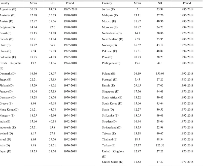
indices, as well as the World Index. The time period considered is December 1970 to December 2018, end of month data for the majority of the indices. From the 49 market indices, 24 Indices are developed markets and 25 are classified as emerging markets taking into consideration the latest market classification from MSCI. While the majority of the developed markets has data available since December 1970, we only have data available for the majority of emerging markets from December 1987 onwards as can be seen in Table I. As for the benchmark, or “Market Return”, the MSCI World Total Return Index in US dollars (World Index) was used as a proxy. The biggest advantage of using MSCI indices, which are composed by large capitalization companies and frequently traded stocks, is that it is unlikely to incur in the bid-ask spread bias as referred by Richards (1997). As for the risk-free rate, the monthly risk-free rate for the US was not available for the entire period of this study. In order to have data for the whole period, we used Bloomberg to collect data regarding the 3-month risk-free rate from the US Yield Curve, and afterwards calculate the effective monthly rate. Such approach was done by Dissanaike (199) as way to bypass the monthly data restriction. As can be seen in Table I, the average annual return for our sample is 15.41%, and the highest average annual return is approximately 36.19% in Poland. Meanwhile, the annual average return on Developed Markets is 13.43%, lower than the annual average return of 18.48% in Emerging Markets. Nevertheless, this higher performance bears higher risk. The standard deviation of the annual returns in Developed markets is around 31.4% while in Emerging Markets it’s 59.06%

2_{Except for the MSCI indices of Brazil, China, Japan, India, Russia and UK which were downloaded}

(16)

Table I. MSCI Indices Annual Returns

Country Mean SD Period Country Mean SD Period

Argentina (E) 30.03 84.33 1987- 2018 Jordan (E) 5 25.98 1987-2018

Australia (D) 12.28 25.73 1970-2018 Malaysia (E) 13.11 37.76 1987-2018

Austria (D) 12.87 37.56 1970-2018 Mexico (E) 21.87 40.96 1987-2018

Belgium (D) 14.24 27.6 1970-2018 Morocco (E) 10.82 24.73 1994-2018

Brazil (E) 21.15 51.78 1998-2018 Netherlands (D) 14.1 20.86 1970-2018

Canada (D) 10.91 21.84 1970-2018 New Zealand (D) 9.78 25.95 1987-2018

Chile (E) 18.72 36.9 1987-2018 Norway (D) 16.52 43.12 1970-2018

China (E) 7.74 39.03 1992-2018 Pakistan (E) 15.31 48.82 1992-2018

Colombia (E) 18.25 44.83 1992-2018 Peru (E) 20.73 38.23 1992-2018

Czech Republic (E)

13.2 31.36 1994-2018 Philippines (E) 15.6 42.1 1987-2018

Denmark (D) 16.36 28.07 1970-2018 Poland (E) 36.19 150.04 1992-2018

Egypt (E) 22.21 55.13 1994-2018 Portugal (D) 5.45 27.25 1987-2018

Finland (D) 15.59 44.02 1987-2018 Russia (E) 29.65 67.05 1998-2018

France (D) 13.04 27.13 1970-2018 Singapore (D) 17.56 44.61 1970-2018

Germany (D) 13.28 28.74 1970-2018 South Africa (E) 13.22 30.43 1992-2018

Greece (E) 8.08 45.68 1987-2018 South Korea (D) 15.66 45.64 1987-2018

Hong Kong (D) 21.21 43.78 1970-2018 Spain (D) 12.27 30.55 1970-2018

Hungary (E) 18.55 42.96 1994-2018 Sri Lanka (E) 13.05 49.01 1992-2018

India (E) 15.66 40.18 1992-2018 Sweden (D) 16.94 28.66 1970-2018

Indonesia (E) 25.51 65.8 1987-2018 Switzerland (D) 13.55 22.98 1970-2018

Ireland (D) 8.17 27.4 1987-2018 Taiwan (E) 13.38 40.67 1987-2018

Israel (D) 8.03 27.76 1992-2018 Thailand (E) 18.5 48.34 1987-2018

Italy (D) 9.88 34.21 1970-2018 Turkey (E) 37.37 122.56 1987-2018

Japan (D) 13.25 31.74 1970-2018 United Kingdom (D)

12.87 27.23 1970-2018

United States (D) 11.52 17.37 1970-2018 The annual returns are expressed in percentage. (D) stands for Developed Markets, while (E) stands for Emerging

Markets.

Figure 1 shows us the evolution of a hypothetical investment of $10,000 in both markets, from December 1987 through December 2018, compounding the monthly average returns in either market. According to our expectations, the value at the end of the period would be higher for emerging markets. While an investment of $10,000 in developed markets would mean a final value of $57,331, that same investment in emerging markets would mean a final value of $100,540.

(17)

Figure 1. Growth of hypothetical $10,000 by market 2.1. Methodology for Excess Returns

Every 3 and 5 years the Indices’ holding periods returns (HPR) were calculated using Equation (1) below:

𝐻𝑃𝑅𝑖,𝑡=_{𝐼𝑛𝑑𝑒𝑥 𝑃𝑟𝑖𝑐𝑒}𝐼𝑛𝑑𝑒𝑥 𝑃𝑟𝑖𝑐𝑒𝑖,𝑡

𝑖,𝑡−𝑘− 1 (1) Where 𝐻𝑃𝑅5,6 represents the holding period return of index i at year t, 𝐼𝑛𝑑𝑒𝑥 𝑃𝑟𝑖𝑐𝑒5,6 stands for the Index Price in USD dollars of Index i at year t, and 𝐼𝑛𝑑𝑒𝑥 𝑃𝑟𝑖𝑐𝑒_5,678 stands for the Index Price in USD dollars of Index i 3, or 5 years, before year t. Despite using market indices data, there is still a benchmark, in this case that benchmark is the MSCI World Index. For simplicity we will call the excess market return as “Excess Return” and it will represent the difference between the HPR of market index i and the World Index’s HPR. All in all, the Excess Returns (ER) were obtained using Equation (2) below:

𝐸𝑅𝑖,𝑡= 𝐻𝑃𝑅𝑖,𝑡− 𝑊𝐼𝑅𝑡 (2) where 𝐸𝑅_5,6 is Excess Return of Index i at year t, 𝐻𝑃𝑅_5,6 is the HPR of Index i at year t; 𝑊𝐼𝑅₆ represents the HPR of the World Index at year t. The indices were then ranked as losers or winners based on their 3- or 5-years excess returns using the quartiles criteria in what’s known as the ranking period. In other words, the indices that had the lowest ER, an ER that belongs in the 1st_{quartile of the excess returns’ distribution, were classified as}

losers. Afterwards, a portfolio solely composed of losers was created. Whereas the indices

0 20,000 40,000 60,000 80,000 100,000 120,000 140,000 160,000 180,000 1988 1989 1990 1991 1992 1993 1994 1995 1996 1997 1998 1999 2000 2001 2002 2003 2004 2005 2006 2007 2008 2009 2010 2011 2012 2013 2014 2015 2016 2017 Va lu e in U SD Emerging Developed

(18)

with the highest ER in the ranking period, which belong in the ranking period 4th_quartile

distribution, were classified as winners and a portfolio only composed of winners was created. The Excess Returns of both portfolios, and also of the contrarian portfolio (difference between losers’ excess returns and winners’ excess returns) was then calculated in the subsequent 3 or 5 years, respectively, which is called the test period. Portfolios had an equal weighting scheme, hereafter their excess returns were calculated according to equation (3):

𝐸𝑅_𝑝,𝑡=∑𝑛𝑖=1_𝑛𝐸𝑅𝑖,𝑡 (3) 𝐸𝑅𝑝,𝑡 is the Excess Return of the respective Portfolio at year t; 𝐸𝑅𝑖,𝑡 is the Excess Return of Index i at year t, while 𝑛 stands for the number of Indices that were included in Portfolio p at the ranking year. Since we used non-overlapping periods this allowed us to repeat this process 15 times for 3-year periods, with the first ranking taking place at December 1973, and the respective first test period ending at December 1976. Taking in consideration the findings from (Chen and Sauer, 1997) we thought it would be useful, and cautious, to split the whole time-period into subperiods. Therefore, we divided into two subperiods. The first subperiod has observations from the years 1970-1997 and the second subperiod has observations from 1998-2018. By doing this, not only do we have two different subperiods with a similar number of test periods (8 in the 1st_{one and 7 in}

the 2nd_{one), but we also have periods with similar number of crisis. In the case of the 1}st

subperiod it includes the late 1980’s Japanese asset bubble, the 1987 Black Monday, while in the 2nd_{subperiod we have the late 90’s Asian tiger crisis, the early 2000’s}

Dot-com bubble and the global financial crisis of 2007-2009. With 5-year periods and also with non-overlapping data, we were able to repeat this process 8 times, with the first ranking taking place at December 1975 and the respective first test period ending at December 1980. Creating subperiods with 5-year investment periods would mean too few observations in each one. As an alternative, we considered the case where 5-year periods would be ranked for the first time in 1978, which would include data from 2016, 2017 and 2018 to see if that would have an impact in our results. Unlike what was done by De Bondt and Thaler (1985), we used BH measures. First, as exposed by Dissanaike (1994) BH returns translate into lower transactions costs and are less exposed to infrequent

(19)

lead to upward biases as concluded by Conrad and Kaul (1993). Although predominantly studied for 3-year periods, there is also evidence for overreaction for 5-year periods in the US and South Korean Markets as stated by De Bondt and Thaler (1985) and Wt Leung and li (1998) respectively. Henceforth, we thought reasonable to study both 3- and 5-year periods. According to the overreaction hypothesis losers’ excess return will be greater than zero ( 𝐸𝑅𝐿,𝑡 > 0), while winners should have negative excess returns (𝐸𝑅𝑊,𝑡< 0 ). This implies that the contrarian portfolio, also called contrarian strategy, should deliver even greater excess returns than losers’ excess returns (𝐸𝑅𝐿−𝑊,𝑡> 0).

2.2. Methodology for Risk-Adjusted Returns

In order to test if the return reversals are a result of overreaction or the risk-reward of losers’ indices, we had to calculate the monthly risk-adjusted returns of the winners and losers based on Dissanaike (1997) with the appropriate modifications. After ranking the indices and creating a portfolio of winners, losers and the contrarian as explained in Chapter 2.1. Methodology for Excess Returns, the portfolio’s monthly returns will be computed in the subsequent 36 months, in the case of 3-year periods, or 60 months in the case of 5-year periods. Afterwards, following the CAPM methodology regressions (4), (5) and (6) will be run for the test periods:

𝑅𝐿,𝑡− 𝑅𝑓,𝑡= 𝛼𝐿,𝑡+ 𝛽_𝐿,𝑡G𝑅𝑊𝐼,𝑡− 𝑅𝑓,𝑡H+ 𝑒𝑡 (4) 𝑅_𝑊,𝑡− 𝑅_𝑓,𝑡= 𝛼_𝑊,𝑡+ 𝛽_𝑊,𝑡G𝑅_{𝑊𝐼,𝑡}− 𝑅_𝑓,𝑡H+ 𝑒_𝑡 (5) 𝑅𝐿−𝑊,𝑡− 𝑅𝑓,𝑡= 𝛼𝐿−𝑊,𝑡+ 𝛽_{𝐿−𝑊,𝑡}G𝑅𝑊𝐼,𝑡− 𝑅𝑓,𝑡H+ 𝑒𝑡 (6) 𝑅L,6 and 𝑅M,6 are the monthly returns of the losers and winners’ portfolios respectively for month t; 𝑅L7M,6 is the monthly return of the contrarian portfolio for month t; 𝑅N,6 is the monthly risk-free rate for month t; 𝑅MO,6 is the monthly return of the MSCI World Total Return Index for month t; 𝛼L, 𝛼M and 𝛼L7M are the constants of the regression which express the monthly abnormal returns of the portfolios. If the weak form of the EMH holds, the alphas should equal zero, since investors can’t be able to use historical data to create profitable investment strategies. In other words, an investor that uses the contrarian strategy shouldn’t be able to systematically get abnormal returns. However, if the overreaction hypothesis holds, an investor that uses the contrarian strategy will be

(20)

able to systematically have abnormal returns. Thus, we should observe the following conditions: 𝛼L>0, 𝛼M<0 and 𝛼L7M>0. 𝛽L,6 and 𝛽M,6 are the betas of the losers and winners’ portfolios, respectively, for month t; while 𝛽L7M,6 represents the contrarian portfolio beta. If losers are less risky than winners, when we run regression (6) the contrarian portfolio’s beta should be, on average, smaller than zero (𝛽L7M,6<0). Unlike the case for excess returns, when we compute the monthly risk-adjusted returns we also have enough observations to split into two subperiods the observations from 5-year periods. Thus, in the case of 3-year periods we have the previously mentioned subperiods. The 1st_{one is 1970-1997 and the 2}nd_{one is 1998-2018. In the case of 5-year periods the}

1st_{subperiod ranges from 1970-1995, and the 2}nd_{subperiod from 1996-2015.}

3. Excess Returns 3.1. 3-year periods

On Table II we can see the effectiveness of the contrarian strategy during each test period 1, 2 and 3 years after the ranking year. In 10 out of 15 test periods losers’ 3-year excess returns are higher than the winners’ excess returns. Moreover, we can also highlight two things. First, losers outperformed winners in almost every test period till the late 90’s, excluding the first test period (1974-1976). Considering the most recent test periods, 1998 onwards, losers only outperformed winners in 3 out of 7 test periods. Still, in the 2013-2015 test period both portfolios had a negative excess return. Second, both portfolios seem to build their excess returns till the end of the test period. This is clearer when we look at the 1983-1985 and 1995-1997 test periods.

Table II. Contrarian Strategy success

Losers Winners

Test Period Year 1 Year 2 Year 3 Year 1 Year 2 Year 3

1974-1976 -7.66 -2.96 -17.00 -9.84 -13.84 -10.63 1977-1979 -13.65 -2.16 40.14 9.05 14.39 12.52 1980-1982 3.39 21.06 8.89 -0.08 -8.45 -36.16 1983-1985 4.07 10.27 75.75 16.38 -10.42 -20.74 1986-1988 -18.93 -32.2 -29.16 8.81 -33.26 -43.30 1989-1991 34.12 52.02 38.28 -2.3 -4.4 -5.33

(21)

1992-1994 -1.22 26.32 35.53 4.47 51.74 20.12 1995-1997 -13.82 -6.91 20.47 -11.52 -18.41 -61.89 1998-2000 -28.88 -4.43 -39.50 -13.48 -17.74 -22.16 2001-2003 23.55 65.87 131.11 -0.86 1.16 10.11 2004-2006 6.81 18.88 43.56 30.61 86.15 113.19 2007-2009 14.77 4.69 14.94 22.61 -4.62 19.64 2010-2012 -6.53 -22.82 -28.67 15.8 1.33 4.52 2013-2015 -9.11 -23.95 -31.34 -23.98 -24.58 -36.04 2016-2018 12.19 24.55 17.42 -6.98 -8.67 -21.12

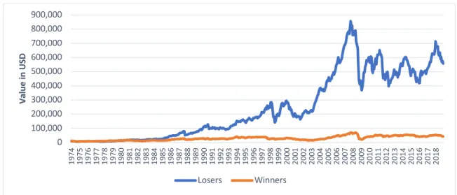
On Figure 2 we get to see how an investment of $10,000 in both portfolios would behave. Compounding the monthly returns of both portfolios we see that both portfolios’ value is quite similar until 1983, the first year of one of the most successful test periods for losers. Nevertheless, there would be some drawdowns in 1987, 1998, 2000, 2008 for both portfolios which had more impact in the losers’ portfolios. All these years represent financial crisis. For instance, in 1998 losers’ portfolio was especially affected by the Asian financial crisis since 6 of the loser indices were South Korea, Indonesia, Philippines, Singapore, Malaysia and Thailand. Also, the 2008 drawdown can be explained in part by the financial crisis of 2007-2008, especially when we consider that the US Index was a loser index in the 2007-2009 test period.

Figure 2. Growth of hypothetical $10,000

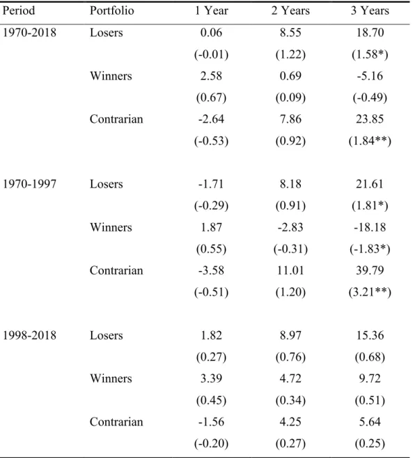
Table III presents the Excess returns for 3-year periods for losers, winners and the contrarian portfolio. The contrarian portfolio yields, on average, an excess return of 23.85% and statistically significant at a 5% significance level (t-stat = 1.84). Furthermore,

0 100,000 200,000 300,000 400,000 500,000 600,000 700,000 800,000 900,000 1974 1975 1976 1977 1978 1979 1980 1981 1982 1983 1984 1985 1986 1987 1988 1989 1990 1991 1992 1993 1994 1995 1996 1997 1998 1999 2000 2001 2002 2003 2004 2005 2006 2007 2008 2009 2010 2011 2012 2013 2014 2015 2016 2017 2018 Va lue in U SD Losers Winners

(22)

while losers provide a 3-year excess return of almost 19%, winners only underperform the market by roughly 5 percentage points, which imply that returns’ reversals might be asymmetrical. In the first subperiod, contrarian portfolio’s excess return is close to 40%, and statistically significant at a 5% significance level (t-stat = 3.21).

Table III. Excess Returns (3-y Ranking)

Period Portfolio 1 Year 2 Years 3 Years

1970-2018 Losers 0.06 (-0.01) 8.55 (1.22) 18.70 (1.58*) Winners 2.58 (0.67) 0.69 (0.09) -5.16 (-0.49) Contrarian -2.64 (-0.53) 7.86 (0.92) 23.85 (1.84**) 1970-1997 Losers -1.71 (-0.29) 8.18 (0.91) 21.61 (1.81*) Winners 1.87 (0.55) -2.83 (-0.31) -18.18 (-1.83*) Contrarian -3.58 (-0.51) 11.01 (1.20) 39.79 (3.21**) 1998-2018 Losers 1.82 (0.27) 8.97 (0.76) 15.36 (0.68) Winners 3.39 (0.45) 4.72 (0.34) 9.72 (0.51) Contrarian -1.56 (-0.20) 4.25 (0.27) 5.64 (0.25)

Excess Returns are expressed in percentage. T-statistic is in parenthesis. The symbols *, and **, indicate the results that are statistically significant for a 10% and 5% significance level and considering a one-tailed test.

While with the whole time period we can observe asymmetric return reversals, in the 1st

subperiod the return reversals are quite similar, and losers’ excess returns are higher. The results in the 2nd_{subperiod are considerably different than the ones in the 1}st_subperiod.

(23)

The contrarian portfolio has, on average, an excess return of 5.64% and statistically non-significant (t-stat = 0.68). This contrast between the 1st_{and the 2}nd_{subperiod excess}

returns for the contrarian portfolio are mainly due to the winners’ performance. While losers still outperform the world index, winners also outperform the world index in this period. The overreaction hypothesis seems to hold in the 1st_{subperiod with statistically}

significant results in accordance with the early findings on equity indices of Richards (1997). On the other hand, in the 2nd_{subperiod there isn’t evidence confirming the}

overreaction hypothesis. Table IV presents the excess returns if we invest exclusively in developed markets and using 3-year periods for ranking and test periods. Considering the whole time period, 1970-2018, the contrarian portfolio provides strong and statistically significant results at a 5% significance level 3 years after the ranking period with an excess return of 19.72% (t-stat = 2.14). Although strong and statistically significant, the contrarian portfolio’s excess returns are slightly less than the ones observed when all the indices were considered. This is mainly due to the lower excess returns that losers have in developed markets. Again, losers and winners’ excess returns seem to be asymmetrical. In the 1st_{subperiod, 1970-1997, the contrarian portfolio provides, on average, an excess}

return of 36.04% which is statistically significant at a 5% significance level (t-stat = 3.21). Besides that, both the winners and loser’s portfolio excess returns are statistically significant at 10% significance level in the 1st_{subperiod. Such results don’t differ much}

from the ones when all the indices where considered, but they are smaller.

Table IV. Excess Returns in Developed Markets (3-y ranking)

Period Portfolio 1 Year 2 Years 3 Years

1970-2018 Losers -0.16 (-0.05) 7.94 (1.33) 13.72 (1.72*) Winners 2.37 (0.86) -3.31 (-0.60) -5.99 (-0.77) Contrarian -2.53 (-0.58) 11.25 (1.63*) 19.72 (2.14**) 1970-1997 Losers -1.52 (-0.26) 7.82 (0.93) 20.96 (1.75*)

(24)

Winners 2.95 (0.96) -3.66 (-0.48) -15.08 (-1.73*) Contrarian -4.47 (-0.63) 11.48 (1.24) 36.04 (3.21**) 1998-2018 Losers 1.39 (0.47) 8.08 (0.88) 5.45 (0.53) Winners 1.70 (0.34) -2.90 (-0.33) 4.39 (0.34) Contrarian -0.31 (0.98) 10.98 (0.98) 1.07 (0.09)

Excess Returns are expressed in percentage. T-statistic is in parenthesis. The symbols *, and **, indicate the results that are statistically significant for a 10% and 5% significance level considering a one-tailed test.

In the 2nd_{subperiod, 1998-2018, the results are considerably different than the ones we}

had with the 1st_{subperiod. As observed with the whole sample, we verify the same trend}

when we invest solely in developed markets. The contrarian portfolio excess returns 3 years after the ranking are close to zero. Again, both losers and winners have positive excess returns. While the results seem to confirm the Overreaction Hypothesis in developed markets for the 1st_{subperiod, with strong and statistically significant results,}

the overreaction hypothesis doesn’t seem to hold in the 2nd_{subperiod. For a proper}

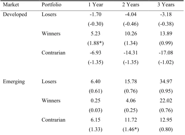
comparison between developed and emerging markets, we framed the time period between 1987 and 2017 since data for emerging markets was only available from December 1987 onwards. Afterwards, we applied the contrarian strategy separately to developed and emerging markets. This procedure was only performed for 3-year periods. Using 5-year periods would translate in too few observations. The first ranking took place in December 1990, which allowed us to repeat this process 9 times with the last test period ending in 2017. As can be seen on Table V, the contrarian portfolio 3-year excess return is, on average, -17.08% in developed markets unlike what would be expected under the overreaction hypothesis. The results don’t seem to confirm the overreaction hypothesis in developed markets for this time period.

(25)

Table V. Excess Returns by Market (3-y ranking)

Market Portfolio 1 Year 2 Years 3 Years

Developed Losers -1.70 (-0.30) -4.04 (-0.46) -3.18 (-0.38) Winners 5.23 (1.88*) 10.26 (1.34) 13.89 (0.99) Contrarian -6.93 (-1.35) -14.31 (-1.35) -17.08 (-1.02) Emerging Losers 6.40 (0.61) 15.78 (0.76) 34.97 (0.95) Winners 0.25 (0.03) 4.06 (0.25) 22.02 (0.76) Contrarian 6.15 (1.33) 11.72 (1.46*) 12.95 (0.80)

Excess Returns are expressed in percentage. T-statistic is in parenthesis. The symbols *, and **, indicate the results that are statistically significant for a 10% and 5% significance level, considering a one-tailed test.

As for the emerging markets, the contrarian portfolios’ excess return is, on average, 12,95% though statistically non-significant (t-stat = 0.80). Also, while there seems to exist overreaction for losers, but the excess returns are not statistically significant, winners also have positive excess returns. Such findings do not allow us to support the Overreaction hypothesis for emerging markets in this time-period. If anything, there seems to exist overreaction for losers’ indices, but only in emerging markets, and as such the only viable strategy would be to invest in them. Additionally, the same strategy was applied to the time period 1988-2018 and the conclusions for emerging markets were different. In this scenario the contrarian portfolio would yield, on average, a 3-year excess return of 37.31% and also statistically significant at a 10% significance level (t-stat = 1.65), since the winners would have a 3-year excess return of -2%.

(26)

3.2. 5-year periods

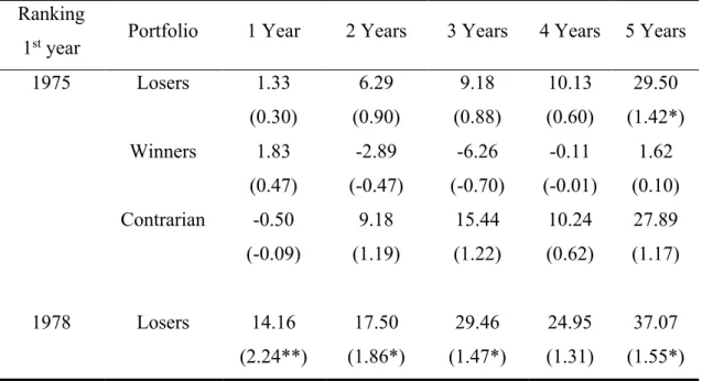
As explained before, in some literature there is evidence of overreaction up to 5 years after the ranking of losers and winners. Table VI presents the results for 5-year test periods taking into consideration the case where the 1st_{ranking takes place in 1975, and}

a scenario where the 1st_{ranking takes place in 1978 as explained before in Chapter 2.1.}

Methodology for Excess Returns.

Table VI. Excess Returns (5-y ranking)

Ranking

1st_year Portfolio 1 Year 2 Years 3 Years 4 Years 5 Years

1975 Losers 3.25 (0.59) 10.64 (1.07) 15.95 (0.86) 26.34 (1.02) 52.63 (1.25) Winners 0.25 (0.07) -4.51 (-0.52) -11.78 (-0.91) -3.98 (-0.22) 1.52 (0.07) Contrarian 2.99 (0.51) 15.15 (1.42) 27.73 (1.52*) 30.22 (1.22) 51.11 (1.28) 1978 Losers 16.65 (2.63**) 20.69 (1.93**) 35.86 (1.81*) 37.34 (1.84*) 43.25 (1.86*) Winners -0.72 (-0.11) 1.56 (0.11) -6.39 (-0.36) 0.38 (0.01) -23.59 (-1.00) Contrarian 17.37 (2.31**) 19.13 (1.12) 42.24 (1.42) 36.96 (1.05) 66.84 (1.81*)

Excess Returns are expressed in percentage. T-statistic is in parenthesis. The symbols *, and **, indicate the results that are statistically significant for a 10% and 5% significance level considering a one-tailed test.

Assuming the 1st_{ranking takes place in 1975, the contrarian portfolio would yield, on}

average, a 5-year excess return of 51.11% but statistically non-significant (t-stat = 1.28). Meanwhile, the 3-year excess returns would be statistically significant at a 10% significance level (t-stat = 1.52). While there is evidence of loser’s overreaction when we consider 5-year periods, the results are not statistically significant. Yet, if the 1st_ranking

takes place in 1978 not only excess returns are higher, but we also have statistically significant results. The contrarian portfolio’s excess return would be, on average, 66.84%

(27)

and statistically significant at a 10% significance level (t-stat = 1.81). Also, winners would have, on average, a 5-year excess return of -23.59% instead of 1.52%. Although considerably high these results express the high values demonstrated by some of the indices. For instance, in the 1999-2003 test period the contrarian portfolio’s excess return was 84.73%, with 4 out the 11 losers indices yielding an excess return of 100% or higher during that test period. At Table VII we can observe the excess returns for 5-year test periods on developed markets. When the 1st_{ranking takes place in 1975 the contrarian}

portfolio yields, on average, a 5-year excess return of 27.89% which is statistically non-significant (t-stat = 1.17). The contrarian portfolio excess returns are considerably smaller when compared with the whole sample 5-year excess return of 51.11% seen on Table VI, mainly due to losers’ smaller excess returns. When the 1st_{ranking takes place in 1978 not}

only excess returns are higher, as previously seen with the whole sample, but we have statistically significant results. The contrarian portfolio 5-year excess return is, on average, 51.39% instead of 27.89%, and statistically significant at a 10% significance level (t-stat = 1.42). As verified with 3-year excess returns, the 5-year excess returns of the contrarian portfolio in developed markets are smaller than the ones verified for the contrarian portfolio when we considered both developed and emerging markets. These results seem to confirm the overreaction hypothesis for 5-year periods. However, the results are only statistically significant when the 1st_{ranking takes place in 1978.}

Table VII. Excess Returns in Developed Markets (5-y ranking)

Ranking

1st_year Portfolio 1 Year 2 Years 3 Years 4 Years 5 Years

1975 Losers 1.33 (0.30) 6.29 (0.90) 9.18 (0.88) 10.13 (0.60) 29.50 (1.42*) Winners 1.83 (0.47) -2.89 (-0.47) -6.26 (-0.70) -0.11 (-0.01) 1.62 (0.10) Contrarian -0.50 (-0.09) 9.18 (1.19) 15.44 (1.22) 10.24 (0.62) 27.89 (1.17) 1978 Losers 14.16 (2.24**) 17.50 (1.86*) 29.46 (1.47*) 24.95 (1.31) 37.07 (1.55*)

(28)

Winners -0.71 (-0.12) -0.35 (-0.04) -8.33 (-0.67) -6.26 (-0.33) -14.32 (-0.88) Contrarian 14.88 (1.80*) 17.85 (1.07) 37.79 (1.27) 31.21 (0.95) 51.39 (1.42*)

Excess Returns are expressed in percentage. T-statistic is in parenthesis. The symbols *, and **, indicate the results that are statistically significant, for a 10% and 5% significance level considering a one-tailed test.

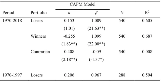
4. Risk-adjusted Returns 4.1. 3-year periods

On Table VIII it is presented the monthly risk-adjusted returns of the 3-year test periods. As it was done for excess returns, we also took in consideration the results for the two subperiods. Losers’ and winners’ alphas signs confirm the overreaction hypothesis. The contrarian portfolio monthly alpha is around 0.408% and statistically significant at a 5% significance level (t-stat = 2.18). Risk doesn’t seem to explain the reversals since the contrarian’s beta is around -0.09 and statistically significant at a 10% significance level (t-stat = -1.37). In other words, losers are less risky than winners. In the 1st_subperiod

losers and winners’ monthly alphas seem to support the overreaction hypothesis. The contrarian portfolio’s alpha is almost 0.79%, and statistically significant at a 5% significance level (t-stat = 3.00). The contrarian portfolio’s beta is still negative which means that losers are less risky than winners.

Table VIII. Risk-Adjusted Returns (3-y ranking)

CAPM Model Period Portfolio α β N R2 1970-2018 Losers 0.153 (1.01) 1.009 (21.63**) 540 0.605 Winners -0.255 (1.83**) 1.099 (22.00**) 540 0.687 Contrarian 0.408 (2.18**) -0.09 (-1.37*) 540 0.008 1970-1997 Losers 0.206 0.967 288 0.594

(29)

(1.04) (12.47) Winners -0.581 (-2.68**) 0.99 (17.36) 288 0.594 Contrarian 0.787 (3.00**) -0.026 (-0.28) 288 0.001 1998-2018 Losers 0.038 (0.16) 1.06 (18.84) 252 0.613 Winners -0.022 (-0.12) 1.197 (15.24) 252 0.774 Contrarian 0.06 (0.22) -0.137 (-1.47*) 252 0.02

The regressions follow the methodology of equations (4), (5) and (6). The robust option was used in Stata, so that the standard-errors of the t-statistics would account for the possibility of heteroskedasticity in residuals’ distribution in accordance with White (1980). The alphas are expressed in percentage. T-statistic is in parenthesis. The symbols *, and **, indicate the results that are statistically significant for a 10% and 5% significance level and considering a one-tailed test.

In the 2nd_{subperiod the contrarian portfolio’s alpha is still greater than zero, 0.06%, but}

substantially smaller than the one observed in the 1st_{subperiod and statistically}

non-significant (t-stat = 0.22). Despite being riskier in the 2nd_{subperiod, losers are still less}

risky than the winners’ portfolio as the contrarian portfolio beta decreased to around -0.137, and also statistically significant at a 10% significance level (t-stat = -1.47). While there is evidence of overreaction, these results are only economically strong and statistically significant in the 1st_{subperiod. Such results highlight the possibility that the}

overreaction hypothesis might not be time stationary as previously referred by (Chen and Sauer, 1997). Considering only the developed markets, the risk-adjusted returns can be found on Table IX. When the contrarian strategy is applied only in developed markets the overreaction hypothesis seems to hold as well. Contrarian portfolio’s monthly alpha is, on average, 0.346% and statistically significant at 5% significance level (t-stat = 2.01), with losers and winners’ alphas’ signs according to the overreaction hypothesis. When compared with the whole sample, in Table VIII, we can observe that the monthly alpha of the contrarian portfolio is slightly smaller in developed markets. Losers are still less

(30)

risky than winners as demonstrated by the contrarian portfolio beta of -0.122, which is statistically significant at a 5% significance level (t-stat = -1.97).

Table IX. Risk-Adjusted Returns in developed markets (3-y ranking)

CAPM Model Period Portfolio α β N R2 1970-2018 Losers 0.161 (1.26) 1.019 (24.61**) 540 0.686 Winners -0.186 (-1.48*) 1.142 (26.57**) 540 0.744 Contrarian 0.346 (2.01**) -0.122 (-1.97**) 540 0.0167 1970-1997 Losers 0.188 (0.96) 0.962 (12.33**) 288 0.601 Winners -0.459 (-2.32**) 1.006 (19.15**) 288 0.654 Contrarian 0.647 (2.48**) -0.044 (-0.49) 288 0.002 1998-2018 Losers 0.055 (0.33) 1.085 (29.44**) 252 0.774 Winners -0.049 (-0.31) 1.274 (20.63**) 252 0.83 Contrarian 0.104 (0.45) -0.189 (-2.38**) 252 0.049

(31)

whole sample’s alpha of 0.787% seen on Table VIII. Winners do seem to be the driver of the contrarian portfolios’ monthly alpha given their average value of -0.459% and statistically significant at a 5% significance level (t-stat = 2.32). In the 2nd_{subperiod we}

notice the same phenomenon as the one observed with the whole sample. Contrarian portfolio’s monthly alpha is positive, but substantially smaller, 0.104% instead of 0.647% as verified in the 1st_{subperiod, and statistically non-significant (t-stat = 0.45). Winners}

are still riskier than losers in the 2nd_{subperiod as demonstrated by the contrarian}

portfolio’s beta of -0.189 which is statistically significant at a 5% significance level (t-stat = -2.38). The results confirm the overreaction hypothesis in developed markets, but only in the 1st_{subperiod. Malin and Bornholt (2013) also found close to zero and}

statistically non-significant alphas in the 2nd_{subperiod of their study for developed}

markets. Nevertheless, while it seems to exist some overreaction in the 1st_{subperiod the}

monthly alphas are considerably smaller and statistically non-significant in the 2nd

subperiod as observed with the whole sample. On Table X we have the risk-adjusted returns when the contrarian strategy is applied separately to developed and emerging markets for the time-period 1987-2017. Unlike what would be expected under the overreaction hypothesis, the contrarian portfolio’s monthly alpha is negative. On average, the monthly alpha of the contrarian portfolio is -0.114% contradicting the overreaction hypothesis. For the emerging markets the results differ. As seen in developed markets, the losers’ monthly alpha is negative, but winners’ alpha is lower. The results appear to display that investors react differently to winners on developed and emerging markets. While in developed markets winners have positive monthly alphas in the test period, in emerging markets winners’ monthly alphas are negative for the time-period considered.

Table X. Risk-Adjusted Returns by Market (3-y ranking)

CAPM Model Market Portfolio α β N R2 Developed Losers -0.049 (-0.31) 1.135 (25.98**) 324 0.738 Winners 0.064 (0.49) 1.21 (25.06**) 324 0.818 Contrarian -0.113 -0.075 324 0.008

(32)

(-0.57) (-1.08) Emerging Losers -0.043 (-0.14) 1.013 (13.52**) 324 0.382 Winners -0.135 (-0.50) 1.088 (12.35**) 324 0.472 Contrarian 0.091 (0.29) -0.076 (-0.94) 324 0.003

4.2. 5-year periods

Table XI presents the monthly risk-adjusted returns when 5-year test periods are used instead of 3-year periods, assuming the 1st_{ranking took place in 1975. While excess}

returns were higher when the 1st_{ranking took place in 1978, for a matter of precaution}

the results used were the ones assuming that the 1st_{ranking took place in 1975. Also,}

given that data for emerging markets indices was only available from December 1987 onwards, these indices were included for the 1st_{time in the 1995 ranking. Therefore, we}

could only apply this strategy to both markets in the 2nd_{subperiod as can be seen on Table}

XI. Contrarian portfolio’s monthly alpha is, on average, 0.541%, and statistically significant at a 5% significance level (t-stat = 2.11). More interesting, not only winners’ monthly alpha is more than twice the one verified for losers, but they are also statistically significant at 5% significance level (t-stat = -1.68). Also, winners appear to be riskier than losers. The contrarian portfolio’s beta is, on average, -0.248 and statistically significant at a 5% significance level (t-stat = -3.64). The results confirm the overreaction hypothesis when 5-y periods are used.

(33)

Table XI. Risk-Adjusted Returns (5-y ranking) CAPM Model Period Portfolio α β N R2 1996-2015 Losers 0.169 (0.83) 1.017 (18.87**) 240 0.677 Winners -0.372 (-1.68**) 1.264 (19.76**) 240 0.739 Contrarian 0.541 (2.11**) -0.248 (-3.64**) 240 0.075

Table XII presents the risk-adjusted returns of the contrarian strategy in developed markets for 5-year periods. The contrarian portfolio has, on average, a monthly alpha of 0.154% which isn’t statistically significant (t-stat = 0.92). Again, differences in risk don’t seem to be the cause for this phenomenon. The contrarian beta is almost -0.17 and statistically significant at a 5% significance level (t-stat = -2.12). In the 1st_subperiod,

losers and winners have an almost symmetrical alpha. On average, the contrarian portfolio’s monthly alpha is around 0.228%, and statistically non-significant (t-stat = 0.86).

Table XII. Risk-Adjusted Returns in developed markets (5-y ranking)

CAPM Model Period Portfolio α β N R2 1970-2015 Losers 0.145 (1.13) 0.998 (16.03**) 480 0.681 Winners -0.009 (-0.06) 1.164 (28.27**) 480 0.752 Contrarian 0.154 (0.92) -0.166 (-2.12**) 480 0.034

(34)

1970-1995 Losers 0.106 (0.52) 0.935 (7.01**) 240 0.576 Winners -0.122 (-0.58) 0.976 (17.85**) 240 0.635 Contrarian 0.228 (0.86) -0.041 (-0.28) 240 0.002 1996-2015 Losers 0.118 (0.71) 1.052 (26.68**) 240 0.773 Winners -0.092 (-0.55) 1.326 (28.35**) 240 0.845 Contrarian 0.21 (0.96) -0.273 (-4.80**) 240 0.119

Meanwhile, in the 2nd_{subperiod the contrarian portfolio would have, on average, a}

monthly alpha of 0.21% which is statistically non-significant (t-stat = 0.96). However, the losers’ portfolio is considerably less risky than the winners’ portfolio in the 2nd

subperiod than in the 1st_{subperiod. As a matter of fact, the contrarian portfolio beta is}

around -0.27 and statistically significant at a 5% significance level (t-stat = -4.80). While there seems to exist overreaction in developed markets for 5-year periods, the results are statistically non-significant. Similar to 3-y periods, the alphas for developed markets are smaller than the ones verified with the whole sample. While the contrarian portfolios’ monthly alpha is, on average, 0.21% in developed markets applying this strategy considering both markets we would have a monthly alpha of 0.541% and statistically significant at a 5% significance level as seen on Table XI.

(35)

Conclusions

The aim of this dissertation was to answer the question: “Do Market Indices overreact?”. The contrarian strategy yields, on average, an excess return of 24%, 3 years after the ranking year. In the 1970-1997 period this excess return would be, on average, 40% and also statistically significant at a 5% significance level clearly confirming the overreaction hypothesis. However, in the 1998-2018 period the results don’t confirm the overreaction hypothesis. While in the 1970-1997 period the contrarian portfolio would have, on average, an excess return of 36.04% and statistically significant at a 5% significance level, this same strategy would have close to zero excess returns in the 1998-2018 period. Such results might indicate that the overreaction hypothesis is not time stationary. Furthermore, when applied solely in developed markets, we found similar results although the excess returns were smaller in the 1st_{subperiod. Risk does not explain the overreaction.}

Contrarian portfolio’s monthly alpha would be 0.787% and statistically significant at a 5% significance level in the 1st_{subperiod, and only 0.06% and statistically non-significant}

in the 2nd_{subperiod. Likewise, when applied in developed markets the contrarian}

portfolio’s monthly alpha would be, on average, 0.647% and statistically significant at a 5% significance level in the 1st_{subperiod. Meanwhile, in the 2}nd_{subperiod the contrarian}

portfolio’s monthly alpha was only 0.104% and statistically non-significant. As such, there seems to exist a difference in overreaction between developed and emerging markets. In fact, when compared directly in the 1987-2017 time-period winners’ alpha in emerging markets were negative unlike what was observed in developed markets. The contrarian’s portfolio beta was always negative regardless of the subperiod and whether or not the strategy was applied to both markets. We also found evidence for overreaction in 5-year periods. On average, the contrarian portfolio would provide an excess return of 51.11% or 66.84% depending on whether the 1st_{ranking took place in 1975 or 1978. Risk}

does not seem to be the cause for the overreaction. The contrarian portfolio’s monthly alpha was 0.541% and statistically significant at a 5% significance level when applied to developed and emerging markets. The contrarian portfolio’s beta was, on average, -0.248 and statistically significant at a 5% significance level. Once again, when we considered only the developed markets in the 1996-2015 time period the monthly alphas were lower as previously seen with 3-year periods. Nevertheless, the contrarian portfolio’s beta was still negative and statistically significant at a 5% significance level.

(36)

Limitations and further research

Notwithstanding these results and conclusions this study still has its limitations. First, the fact that developed and emerging markets have unbalanced observations. Whilst data for the majority of developed markets indices was available since December 1970, the inception date for emerging markets data was December 1987. Second, while Indices’ market capitalization represents the capitalization of their holdings they can be affected by the macroeconomic conditions of their respective countries or trade partners which this study does not reflect. Regarding future research, we consider that the results obtained with the ranking procedure and the portfolio weighting scheme used in this study should be compared with the results obtained with different methodologies. While losers and winners were ranked upon what we call the “quartile criteria” other authors also consider as losers and winners the indices whose past returns belong to the 1st_{and 10}th

decile of the ranking period distribution. For future research it would be interesting to study if the results differ, or not, when deciles are used instead of quartiles to rank losers and winners. Moreover, the concept of the average, 5th_{decile, portfolio should also be}

studied and how it compares with the extreme decile’s portfolios. Another aspect that should be analyzed should be the weighting scheme of the portfolios. As such, it can be interesting to analyze if the weighting schemes have an impact on the overreaction hypothesis. For this matter there are two possibilities. The first one would consist in using a capitalization-weighted scheming, whereas the total market capitalization would be used to compute the weight of each Market Index. The second approach would consist in a double ranking procedure. After ranking the indices and labeling them as losers and winners, the losers and winners would be ranked separately, and their weights would be proportional to their ranking score. In other words, the losers (winners) weights would be equal to the ratio between a loser’s (winners’) ranking and the sum of all losers’ (winners’) rankings. For instance, in a scenario where we would have 10 losers the loser with ranking 10 would have a portfolio weight of 10/55.