UNIVERSITY OF ALGARVE
FACULTY OF SCIENCES AND TECHNOLOGY
SPATIAL VARIABILITY OF MACROINVERTEBRATE ASSEMBLAGES
AND THE INFLUENCE OF HYDROLOGY AND ENVIRONMENTAL
VARIABLES ALONG THE SIGI RIVER, TANZANIA EAST AFRICA.
ERASMUS MUNDUS MASTER OF SCIENCE IN ECOHYDROLOGY
ROSEMARY JOSHUA MASIKINI
FARO
2012
This research was conducted in the framework of the Master Degree in Ecohydrology and submitted to the University of Algarve, Portugal. It addresses the longitudinal variation of macroinvertebrate assemblages as well as the influence of hydrological and environmental variables in their distribution at Sigi River in Tanzania. The research was supported by an ERASMUS MUNDUS scholarship
NOME/NAME: Rosemary Joshua Masikini FACULDADE/FACULTY: Faculty of Science and Technology ORIENTADOR/SUPERVISORS: Prof. Luis Chicharo and Dr. Pedro Range DATA/ DATE: 15 September 2012
TITULO DA TESE/ TITLE OF THESIS: Spatial variability of macroinvertebrate assemblages and the influence of hydrological and environmental variables along the Sigi River, Tanzania East Africa.
ACKNOWLEDGEMENTS
I am very grateful to my first supervisor Prof. Luis Chicharo for his invaluable supervision and guidance. His simplicity and patience inspired me, Muito obrigada. My sincerely appreciation goes to my second supervisor Dr. Pedro Range for his time and patience in directing the data analysis, reading and correcting the manuscript. Special thanks to Ms Lulu Tunu Kaaya for her tireless efforts in directing this thesis since the very beginning to the end. I would like to acknowledge the department of Aquatic sciences and Fisheries (University of Dar es salaam) for providing me space, instruments and identification key books during my laboratory work.
I would like to thanks Pangani river water office in Tanga city Mama Materu, Juma for landing me some instruments and car during my field visit to Sigi River. My appreciation goes to Wami River water office in Morogoro town – Praxeda Kalugendo for allowing taking the hydrological measuring instruments during the sampling events. Great thanks to Elibariki Mmasi (Hydrologist technician) and Anna Mwambala (MSc student at University of Dar es salaam) who accompanied and helped me during the field sampling. The Erasmus Mundus Programme sponsored my Master Studies.
Last but not least, I would like to thanks my family for their love and patience they have always show to me. To God be the glory. I acknowledge His protection, provision and strength throughout my study period.
RESUMO
O estudo de investigar a variabilidade espacial e temporal de macroinvertebrados e sua relação com a hidrologia, fatores hidráulicos e ambientais foi feito ao longo do Rio Sigi durante dois períodos de amostragem na estação seca (Março) e chuvosa (Maio) de 2012. O rio foi demarcada com base nas taxas de inclinação e cinco zonas do rio foram identificadas como: riachos em montanhas, alto sopé, baixo sopé, rejuvenescente sopé e rio inferior. Amostras de macroinvertebrados foram coletadas a partir das cinco zonas fluviais e medições dos parâmetros hidrológicos (descarga), hidráulicos (profundidade, velocidade e número de Froude) e ambientais (pH, temperatura, substrato, condutividade), foram feitas em cada zona.
Ao caracterizar as assembléias de macroinvertebrados ao longo do Rio Sigi, índices de diversidade (número de táxons, abundâncias totais, índice de riqueza de Margalef e Shannon Wiener) foram calculados e as espécies mais representativas foram identificadas para a variação espacial e temporal. Melanoides, Amphypsyche, Elminae e Afronurous mostraram diferenças na abundância em dois períodos amostrados, enquanto Cleopatra, Potamonautes, Ephemerythus, Neoperla, Caenis, Ceratogomphus e Cheumatopsyche apresentaram diferença significativa entre as zonas fluviais. Correlação de Sperman e Modelo de Distância Linear foram usados a fim de revelar os fatores físicos que regem a distribuição da comunidade de macroinvertebrados bentônicos.
O estudo demonstrou que a variação dos factores físicos, como a descarga, temperatura, condutividade e pH apresentam um papel importante na distribuição espacial na comunidade de macroinvertebrados ao longo do rio e do ciclo de vida dos macroinvertebrados (Afronurus) sendo importante para a determinação da variabilidade temporal. Palavrachave: Invertebrados aquáticos, Zonação do rio, variação temporal, Rio Sigi, fatores físicos.
ABSTRACT
The study of investigating the spatial and temporal variability of macroinvertebrate and their relation to hydrology, hydraulic and environmental factors was done along the Sigi River during two sampling periods in the dry (March) and wet (May) periods of 2012.
The river was demarcated based on slope ranges and five river zones were identified as mountains streams (MS), upper foothills (UF), lower foothills (LF), rejuvenated foothills (REJ) and mature lower river (MR). Samples of macroinvertebrate were collected from the five river zones and measurements of hydrological (discharge), hydraulics (Depth, velocity and Froude number) and Environmental (pH, Temperature, substrate, conductivity) parameters were done in each zone.
In characterizing the macroinvertebrate assemblages along the Sigi River diversity indices (number of taxa, total abundances, Margalef richness index and ShannonWiener index) were calculated and the most representative species for the spatial and temporal variation were identified. Melanoides and Afronurous showed differences in abundance in two samplings periods while Cleopatra, Potamonautes, Ephemerythus, Neoperla, Caenis, Ceratogomphus and Cheumatopsyche showed significant difference among the river zones. Spearman rank correlation and Distance Linear Model (DistLM) used to revealed physical factors governing the macroinvertebrate assemblages distribution.
The study demonstrated that the variation of physical factors like discharge, temperature, conductivity and pH have an important role in the spatial distribution of macroinvertebrate assemblages along the river and the life cycle of macroinvertebrate (Afronurus) is important in determining the temporal variability. Keywords: Aquatic invertebrates, River zonation, temporal variation, Sigi River Tanzania, physical factors.
Table of Contents
ACKNOWLEDGEMENTS ... iv ABSTRACT ... vi LIST OF TABLES ... ix LIST OF FIGURES ... x 1.0 INTRODUCTION... 1 1.1 General introduction ... 1 1.2 Spatial and temporal variability of macroinvertebrates assemblages ... 2 1.3 Hydraulics influence on macroinvertebrates assemblages. ... 4 1.4 Aim ... 5 2.0 MATERIALS AND METHODS ... 6 2.1 Study area ... 6 2.1.1 Climate... 6 2.1.2 Geology ... 7 2.1.3 Land cover and activities in the Sigi catchment ... 8 2.2 River Zonation... 9 2.3 Sampling design ... 11 2.4 Macroinvertebrates sampling ... 12 2.5 Hydrological, hydraulics and environmental variables measurements ... 13 2.5.1 Hydrological variables ... 13 2.5.2 Hydraulic variables ... 16 2.5.3 Environmental variables ... 16 2.6 Data Analysis ... 17 2.6.1 Macroinvertebrates Data ... 17 2.6.2 Hydrology, hydraulic and environmental variables ... 19 3.0 RESULTS ... 20 3.1 Diversity indices ... 20 3.2 Macroinvertebrate assemblages ... 22 3.3 Single species analysis ... 28 3.4 Hydrological, hydraulic and environmental variables ... 32
3.5 Macroinvertebrate distribution in relation to hydrology, hydraulic and environmental variables. ... 34 4.0 DISCUSSION ... 37 4.1 Macroinvertebrate comparison among the river zones ... 40 4.2 Macroinvertebrate distribution in dry and wet periods. ... 41 4.3 The influence of Hydrology and Environmental variables ... 42 5.0 ECOHYDROLOGY APPROACH IN SIGI RIVER. ... 44 6.0 CONCLUSION ... 46 REFERENCES ... 47 Appendix ... 56
LIST OF TABLES
Table 1: Showing the longitudinal classification of Sigi River based on stream gradient. 10 Table 2: Sampling sites along the Sigi River with indication of river zones ... 11 Table 3: Macroinvertebrate sampling design and data organisation. ... 12 Table 4: Results of ANOVA based on biotic indices for the five river zones and two sampling periods.. ... 20 Table 5: List of identified taxa of macroinvertebrates in the five zones of Sigi river in dry period. ... 23 Table 6: List of identified taxa of macroinvertebrates in the five zones of Sigi river in wet period.. ... 24 Table 7: Analysis of Similarity among river zones and between the sampling period. .... 26 Table 8: Average contribution of each taxa to the dissimilarities among the river zones for dry and wet periods as determined in SIMPER analysis. ... 27 Table 9: Results of ANOVA test of macroinvertebrate species contributed to the dissimilarity among the river zones.. ... 29 Table 10: Hydrology, hydraulic and Environmental variables in the five zones of Sigi River in the dry period. ... 32 Table 11: Hydrology, hydraulic and Environmental variables in the five zones of Sigi River in the wet period... 32 Table 12: ANOVA test for hydrological, hydraulic and environmental variables ... 33 Table 13: Results of the multivariate Spearman rank correlation of environmental data to macroinvertebrate assemblages data using BIOENV. ... 34 Table 14: dbRDA test of hydrological and environmental variables ... 35
LIST OF FIGURES
Figure 1: The map showing Sigi River Catchment and the sampling stations ... 7 Figure 2: OTT Qliner, A system for mobile discharge measurement in rivers ... 14 Figure 3: OTT Acoustic Digital Current meter ... 14 Figure 4: OTT Signal counter ... 14Figure 5: Diversity indices indicating number of taxa, Total number of individuals, Margalef’s species richness index and ShannonWiener diversity index for the dry and wet seasons.. ... 21 Figure 6: MDS ordination showing the spatial distribution of macroinvertebrate assemblages along Sigi River in dry and wet periods... 25 Figure 7: Abundance of the major taxa contributing to the difference among the river zones and between the two sampling periods.. ... 30 Figure 8: Abundance of the major taxa contributing to the difference among the river zones and between the two sampling periods.. ... 31 Figure 9: RDA plot on species abundances and hydrology and environmental variable in the studied area. ... 36
1.0 INTRODUCTION
1.1 General introduction
Rivers are longitudinal systems that integrate the characteristics of the catchment they drain, are extremely complex ecosystems driven and affected by a multitude of physical and biological factors that interact to generate biotic patterns (Dallas 2004). Due to these interactions, the biological community in rivers exhibits a high degree of spatial and temporal variability (Cooper et al. 1997). Longitudinal variation of the river ecosystems has been associated with the biological distribution down the length of the river. Thus longitudinal zonation of rivers has been widely adopted by ecologist in order to explain the variations in biological distribution (Hawkes 1975, Parsons & Thoms 2007).
The spatial and temporal variability of biological community in particular aquatic macroinvertebrate is a widely studied characteristic in lotic ecosystems (Hawkins et al. 1997). Several studies on aquatic macroinvertebrates have used them as bioindicators for assessing water quality in surface waters, similar studies have been conducted in east Africa and Tanzania (Masese et al. 2009, Masese et al. 2010, Ngupulu & Kayanda 2010). Also macroinvertebrate have been use as indicators in determining the minimum flow (environmental flow assessment) required in rivers of east and southern Africa.
There is strong evidence that aquatic macroinvertebrate distribution is influenced by the physical variables dynamics and processes that occur in the river. These include hydrological dynamics, hydraulics or inchannel processes and environmental changes. Aquatic macroinvertebrate have been reported to be influenced by inchannel physical conditions (Kemp et al. 2000). The study of Gore & Judy (1981) and Rossaro et al. (2006) have described the different curves explaining the preference of many different species of macroinvertebrate for velocity, depth, discharge, Froude number, substrate size, demonstrating that a range of species preferences exists. Other physical factors like water temperature (CamurElipek et al. 2010), conductivity (Mesa 2010), dissolved oxygen (Gabriels et al. 2007), substratum (Goncalves et al. 2004) and channel geomorphology (Woodcock et al. 2006) have also showed to influence the distribution of macroinvertebrate assemblages.
The relative importance of these hydrology and environmental factors varied not only among the region, but also within a region (Park et al. 2007, Song et al. 2007). Hydrological, hydraulic and environmental conditions in a river have been identified by many authors as the best predictive variable of macroinvertebrate distribution (Barmuta 1990, Kemp et al. 2000, Brettler et al. 2012). Although there is a close linkage of these physical factors and macroinvertebrate assemblages but the understanding of how and which variables of hydrology, hydraulics and environmental processes influence the macroinvertebrate assemblages is still less explored, particularly in Tanzania this knowledge is very limited. Understanding the interaction of physical variables and macroinvertebrate assemblages is essential for aquatic ecosystem conservation. Aquatic macroinvertebrate play an important role in the riverine ecosystem as they process detritus and algae and provide food to their aquatic animals therefore understanding their distribution pattern is useful. 1.2 Spatial and temporal variability of macroinvertebrates assemblages The spatial variation of macroinvertebrate community depends on a range of abiotic factors that occur in a catchment, site and within a habiat scales (Wiley et al. 1997, Rowntree & Wadeson 1999). Catchment scale factors include differences in channel slope, climate, geology, altitude, longitude/latitude and distance from the source and upstream catchment (Wright 1995, Bailey et al. 1998, Dallas 2007). Factors operating at the site scale include the width, depth, flow pattern and canopy cover (Wright 1995, Collier et al. 1998, Linke et al. 1999, Dallas 2007). Habitat scale factors include the nature and extent of substrate type, availability of biotopes (Dallas 2007) and hydraulic conditions (Padmore 1998, Kemp et al. 2000).
The River continuum Concept (RCC) by Vannote et al. (1980) explained that species distributions and diversity of macroinvertebrates can display predictable changes from upstream to downstream. For instance, taxonomically related species of macroinvertebrates often show contrasting distributional patterns in relation to stream size (Edington & Hildrew 1990), changes in food availability e.g. allochthonous and autochthonous and diversity peaks
challenging. The gradual change in factors such elevation, water temperature, flow rate and food resources along the longitudinal profile exerts a direct influence on the population dynamics of macroinvertebrates and other organisms, contributing to ecological river zonation. The importance of multiple scale of environmental control in local assemblage organization has been widely known, however still few studies have examined this patterns and processes across spatial scales in streams (Downes et al. 1993, Li et al. 2001).
River systems also show a daily and seasonal periodicity in physical factors. Seasonal and year toyear variability in macroinvertebrates community have been closely linked with the unevenness in precipitation events (McElravy et al. 1989). In tropical regions fluctuations in precipitation which results to variation of the stream discharge, often represent the strongest seasonal variation, and change the environment to an extent comparable to temperature in temperate areas (Flecker & Feifarek 1994, Jacobsen & Encalada 1998). Variations in discharge often give differences in wetted perimeter, hydraulic conditions and biotope availability. For example, in case of stony bottom biotopes may become a riffle in lowflow conditions and as runs in highflow conditions. These changes are closely related to their life history stages such as emergence, feeding and growth that are prompted into them. Temperature is among the important factors that exhibits temporal variation. Water temperature as being a climaticallydriven variable can be controlled by other factors such as discharge, altitude, canopy cover and seasons. The variations in temperature affect the growth and distribution of macroinvertebrates, for instance summer maximum temperature may limit the occurrence of certain species (Hawkins et al. 1997). In a more complex way, seasonal variability may occur longitudinally down a river termed as spatialtemporal interaction, in which upland sites can have a single macroinvertebrate assemblage whilst in lowland sites can have a distinct winter and summer assemblage or a certain group of macroinvertebrate can occur downstream in early months and upstream during the late months (King 1981, Linke et al. 1999).
1.3 Hydraulics influence on macroinvertebrates assemblages.
Hydraulics conditions influence biota directly by exerting stress that will limit access and utilisation of habitat (Davis 1986) and through the influence on the supply of particulate food resources, dissolved gases and nutrients for metabolic processes (Biggs et al. 2005). Water depth, velocity, roughness and slope are the primarily parameters of the hydraulic conditions of the river channel, which usually shows temporal and spatial variations. These parameters may have influence on biota indirectly by modifying, creating and eliminating physical habitat (Biggs et al. 2005). They are recognised significant in determining the macroinvertebrate community organisation (Davis & Barmuta 1989, Carling 1992) by influencing their metabolism feeding and the behaviours (Statzner et al. 1988). However there have been limited studies of the relationship between these variables and macroinvetebrates. Froude number as a complex stream hydraulic variable has proposed among the major variable in influencing the macroinvertebrate assemblages distribution (Grown & Davis 1994, Jowett 1993). The relationship of hydraulic variables and benthic fauna has been found to be negative meaning that lower hydraulic values corresponded to higher benthic fauna abundances and taxonomic richness Brooks et al. (2005). Velocity has been recognised to be the important in determining pattern of macroinvertebrates abundances and diversity (Brooks et al. 2005, Reid & Thomas 2008), accounting for 67%77% of the spatial variation. In the same study depth was found to have a lesser influence on spatial variation on the biodiversity and abundances of benthic fauna. In conclusion, the majority of benthic fauna is generally associated with the areas of lower hydraulic variables, presumably where metabolic requirements were lower and adequate food resources were present. The influence of physical factors ranges with the habitat scale, macrohabitat variation is primary caused by the variation in the hydrological processes like discharges and geomorphic factors (Sheldon & Walker 1998) while in the case of mesohabitat the variation has been related to the longitudinal gradients in discharges, particle size and hydraulic variables (Barmuta 1990, Downes et al. 2000).
1.4 Aim
Main objective of the study
The main aim of this study was to assess the spatial and temporal distribution of macroinvertebrate assemblages at different zones along the Sigi River and its relationship with the hydrological, hydraulics and environmental variables in wet and dry periods. Specific objectives To determine the spatial pattern of the macroinvertebrate assemblages along the Sigi river.
To assess the temporal variations in macroinvertebrate assemblages along the Sigi River during the two sampling periods (dry and wet periods).
To determine the influence of hydrological (discharge), hydraulics (flow velocity, depth and Froude number) and environmental (pH, temperature and conductivity) variables on macroinvertebrate assemblages.
2.0 MATERIALS AND METHODS
2.1 Study area
Sigi River is a perennial water body located in Tanga Region, northeastern of Tanzania Figure 1. The river lies between latitudes 4048´S and 5015´S and longitudes 38034´E and 39003´E with a catchment area of about 1,100km2. It rises in the Amani Nature Reserve in the eastern slopes of the East Usambara Mountains at an altitude of 1130m. Sigi River has two main tributaries flowing from the north (Muzi stream) and south (Kihuhwi stream) and after their confluence it drains eastwards out of Usambaras and north of the city of Tanga into the Indian Ocean via the Mabayani Dam, a source for the Tanga Municipal Water Supply.
The upper reaches of the catchment are mountainous, consisting mainly of dense forest interspersed with tea plantations. Its lower parts are flat and some parts being rejuvenated comprising dry savannahtype bushes and low trees, as well as sisal estates. Along the coast coconut and palm trees are common. 2.1.1 Climate Sigi river catchment is characterized by two rainy seasons (bimodal). March to May is the long rain period while October to December marks the short rains. Occasionally long rains tend to be heavy but the annual average rainfall in Sigi catchment varies between 1000mm to 2000mm (IUCN 2003). These rains contribute in increasing the volume of the Sigi river. The annual mean temperature ranges from 20.8ºC in the mountainous areas to 300C in the lower zones (coastal areas).
Figure 1: The map showing Sigi River Catchment and the sampling stations. 2.1.2 Geology The upper and middle Sigi catchment comprises metamorphic rocks of the Usagaran system that have been migmatised and consist of the pyroxene and hornblende granulites and gneisses. The lower Sigi catchment is made up of a sedimentary succession of rocks from karro to Quaternary in age, from sequence of sand stones and shales giving way to Jurassic marine marls and Tanga limestones while younger Neogene sediments consists mainly of raised coral reef deposits (Hamilton & BenstedSmith 1989). Sigi river basin Tanzania & & # # # ! " " ! % % n m ! n 1 2 3 4 5 6 7 8 9 10 11 Sigi River Catchment 0 5 10 20 Km Rejuvenated foothill # Mountain stream Legend Sampling station River zones ! ( Upper foothill " Lower foothill & Mature river % n m ! n Mabayani dam Gauge station
¯
2.1.3 Land cover and activities in the Sigi catchment Agriculture Agriculture is the main land use in the catchment covers about 617.69 km2 (61,769ha) which account for 56.16% of the total area. Food crops such as maize, cassava, banana and fruit are cultivated, while cash crops such as sisal and tea are very common in the mountainous areas e.g. Derema and Longuza Tea Plantation project. Forests There is 450.99km2 (45,099 ha) of forest in the Sigi Catchment, which include both natural and plantation forests. This account for 41% of the total area. Water
The water in the catchment covers about 21.63 km2 (2.163ha) which is 1.93% of the total area. Also the Sigi River provides domestic water to Tanga Municipality (population 300,000), associated industries, estates and adjacent local communities through the Mabayani dam. The Mabayani dam was constructed in late 1970’s. It is approximately 3,500m long with an average width of 400m. Initially (in 1978), the reservoir had a nominal storage capacity of 7.7 million m3, but this has gradually decreased due to siltation caused by erosion and landslides. Sand Mining This has found to be major land use especially inside the Sigi river at the low land area where the substratum is sand. This has lead to habitat destruction, change of the flow regime e.g. creation of more pools and as the results affecting aquatic organism especially benthic macroinvertebrates which highly depend on the bottom substrate.
Domestic activities
Domestic activities such as washing, bathing are taking place directly in the river channel, this deteriorate the water quality due to addition of nutrients (Phosphate and nitrogen) from detergents and other organic matters. Domestic activities have mainly being observed in the middle zones areas where Sigi River is passing near the villages. Fisheries Fishing is carried out mainly along the coast of Indian Ocean, where the Sigi River’s mouth is to be found. Small fisheries exist along its course, targeting fish such as Clarias sp. (a cat fish, ‘kambare’), Tilapia sp. (‘perege’), Labeo (‘ningu’), Synodontis (‘ngogogo’), Barbus (‘kuyu’) and others. Fishing on the Mabayani reservoir is forbidden because its water is intended as a source of domestic water for the Tanga Municipality.
2.2 River Zonation
Zonation of the Sigi River was derived from analyses of the gradients measured from 1:50,000 topographic map of Sigi catchment. The stream gradient (slope) in each site was calculated as the function of distance and change in elevation. From topographic maps, the stream gradient was calculated as the difference between the upper and the lower contour (contour interval) at each site, dividing by the length of the stream segment (Equation 1). Equation 1: Calculation of stream gradient/slope 𝐒𝐭𝐫𝐞𝐚𝐦 𝐠𝐫𝐚𝐝𝐢𝐞𝐧𝐭 (𝐬𝐥𝐨𝐩𝐞) = ∆ in elevation River segment length
However the gradient scale described for South African rivers by Rowntree & Wadeson (1999) were lower for the Sigi catchment. The slopes ranges were defining a higher longitudinal zone than the actual zones. Longitudinal profiles of some Tanzanian rivers have been interfered due to the tectonic movements through uplifting and rifting. The uplifting and rifting in late Miocene caused rivers to be rejuvenated (Burgess & Clarke 2000). The Pangani rift segments of the Eastern Rift Branch extend their effects to the coast of Indian Ocean and have contributed significantly to the rejuvenation of the Sigi River. Prominent knick points in the Sigi River are associated to the bedrock nature of this catchment. Profiles of rivers incised into bedrock are characterised by prominent knick points even in areas not influenced with uplift, lithology or tributary confluence (Woodford 1951). In this study the gradient scales were modified to reflect the actual profile of study (Table 1) Table 1: Showing the longitudinal classification of Sigi River based on stream gradient. River zones Gradient range Description
Mountain Torrent ≥ 0.2 Mountain streams (MS) 0.1 – 0.1999 Steep gradients, dominated by bedrock, boulders and locally gravel or cobble with pools Upper foothill (UF) 0.050 0.099 Gravel and cobbles: riffles, runs, and pools Lower foothill (LF) 0.005 – 0.049 Wide river, run, sand, silt Lower matured river (MR) ≤ 0.0049 Sand Rejuvenated foothill (REJ)
0.050.2 Sections of the lower river with higher gradient and characteristics of the upper rivers. The channel is bedrock controlled with lateral development of alluvial reach types Bedrock and boulders; cascades, falls, isolated pools
Table 2: Sampling sites along the Sigi River with indication of river zones characteristics. Codes; MS = Mountain streams, UF= Upper foothill, LF= Lower foothill, REJ = Rejuvenated foothill and MR= Lower mature river
Site No Site names Latitude
(S) Longitude (E) Gradient River zones
01 Derema 5.086003 38.64096 0.1225 MS 02 Nenguruwe 5.101836 38.6467 0.1551 MS 03 Bulwa 5.107169 38.64528 0.2033 MS 04 Longuza 5.117764 38.69215 0.0955 UF 05 Sigi Lydia 4.996806 38.72709 0.0623 UF 06 Sigi Darajani 5.011394 38.78616 0.0308 LF 07 Sig Lanconi 5.016944 38.80127 0.0406 LF 08 Sigi KwaMpare 5.017692 38.93521 0.0676 REJ 09 Sigi Kidudumo 5.049761 38.97742 0.0557 REJ 10 Sigi Cross Z 5.058469 39.01421 0.0048 MR 11 Sigi Sega 5.055686 39.04221 0.0050 MR 2.3 Sampling design Macroinvertebrates were sampled at 11 sites along the Sigi River (Figure 1), the sites were selected to represent the different river gradient (Table 2). Two sampling periods were analysed: dry period (March, 5th to 9th 2012) and wet period (May, 25th to 28th 2012). In both sampling periods also river discharge, velocity, depth and environmental parameters (pH, temperature and conductivity) were measured.
In the dry season 9 sampling sites were samples. In order to analyse all river zones, 2 missing sites were sampled during the following wet season making a total of 11 sites, in order to have at least more than 1 site in each of the river zones. In each site 3 replicate were collected which were referred to as samples and were treated separately. In total 60 samples were collected, 27 samples in the dry season and 33 samples in the wet season at 5 river zones (MS, LF, UF, REJ and MR). The samples collected were organised to represent the
five river zones. The substrate was described in each river zone and the following scale was used; Sands = 1, gravels = 2, cobbles = 3, boulders = 4 and Bedrock 5. Substrate was considered as an environmental variable. Table 3 below summarizes the data organisation. Table 3: Macroinvertebrate sampling design and data organisation. River zones No of sites representing Substrate substrate Scale Season Dry Wet MS 3 Boulders 4 9 9 UF 2 Cobbles& gravels 3 6 6 LF 2 sand 1 6 6 REJ 2 Bedrock 5 3 6 MR 2 Sand 1 3 6 2.4 Macroinvertebrates sampling
Qualitative sampling of macroinvertebrates was performed during wet and dry season. In each station the dominant biotope (Stones, sand and vegetation) was identified which was simply the habitat contribute to more than 50% of the area within the selected 50 m reach for sampling. Three replicates samples of macroinvertebrate were collected in the selected biotope. Macroinvertebrates were collected always by the same operator using a 30x30 cm kick net with a 1 mm mesh size and applying time limited samples (3 minutes). Samples were fixed in 80% ethanol, transported to the laboratory where they were rinsed using a sieve of 1 mm mesh size, sorted under magnification and preserved in 70% ethanol. All individuals in a sample were counted and most were identified to the Genus level except few of them to family level (Baetidae, Leptophlebiidae, Polycentropodidae, Polymitarcyidae, Tricorythidae, Veliidae and Hirudinea) and Chironomidae and Elmidae were identified to subfamily level.
2.5 Hydrological, hydraulics and environmental variables measurements
2.5.1 Hydrological variables
River discharge was used as a parameter representing hydrological conditions of the river. Signal counter, ADC (Acoustic Digital Current meter) and Qliner were used in discharge measurements (Figure 2, Figure 3 & Figure 4). In dry period the Signal counter device was used for discharge measurements while in wet period ADC and Qliner were used.
During flow measurements at each sampling station, the measuring tape was stretched between the endpoints of the river channel crosssection. Then the cross section distance was divided into intervals/cells depending on the river width. The cell or interval length was between 1m2m, to make at least 3 cells across the river. At each interval or cells the distance, depth (m) and velocity (m/s) was measured. At low depths (<0.5m) 0.6D velocity measurements were done and at high depth (>0.5m) a 0.8D and 0.2D measurements were done in each cell/interval. To take the reading the rod was held in a vertical position with the meter directly into the flow. The sensor or propeller was kept completely under water, facing into the current (for 30 s) and free of interference. The meter was adjusted slightly up or downstream to avoid boulders, snags and other obstructions.
OTT Qliner was used for hydrological measurements in only two sites due to higher depth (> 1m). The instrument consists of a robust and reliable ultrasound Doppler current profiler, a stable boat to hold the profiler, a Bluetooth transmitter, a watertight handheld (PDA) and the corresponding user software. Using the classical vertical process the Qliner measures both the vertical velocity and the water depth at each interval. All measured data are transferred to the PDA via Bluetooth and processed online. After the measurement is complete, the discharge is available immediately.
Figure 2: OTT Qliner, A system for mobile discharge measurement in rivers Figure 3: OTT Acoustic Digital Current meter (Source: http//www.ott.com)
Computation river discharge.
These computations where done when the signal counter device was used during the spot measurements. Unlike ADC and Qliner, which automatically gives the mean velocity and discharge, Signal counter gave only the revolution time. The equations below were used to calculate the velocities. For small propeller For Large propeller Note: n= number of revolution counted * time (30s) When the section velocity calculation was complete, the river discharge (Q) in each section was calculated as recommended by the U.S. Geological Survey. Area (An) of each subsection was computed by; An= subsection width (Wn)*subsection depth (Dn) The subsection discharge (Qn) was obtained by multiplying the subsection area by its
velocity (mean velocity of the subsection). The calculation was repeated for all cells/subsections. Qn= subsection velocity (Vn)* An The total discharge (Q) was obtained by summing subsections discharge. Q = ∑ (An* Vn) or ∑Qn If n = <1.75; v = 0.0670n+0.018 If 1.79=<n=<9.29; v = 0.0564n+0.037 If 9.29=<n<17.49; v = 0.0536n+0.063 If n = <0.84; v = 0.0670n+0.018 If 0.84=<n=<9.56; v = 0.0564n+0.037
2.5.2 Hydraulic variables
The simple measurements of depth and velocities were used to calculate more complex variables in an effort to better identify the hydraulic microhabitats. The Froude number was used as a complex variable. The below formula was used in calculating Froude number (Newman 1977) Froude number = B √DE Where; v = Mean velocity (m/s) g = Gravitational (10 m/s2) h = Mean water depth (m) 2.5.3 Environmental variables
On each sampling occasion, environmental variables were measured prior to invertebrate sampling and hydrological measurements. Water temperature, pH and conductivity were measured insitu using a multi portable probe.
2.6 Data Analysis 2.6.1 Macroinvertebrates Data Diversity indices Diversity indices which include number of taxa, total abundances, Margalef species richness index (d´) and Shannon diversity index (H´) were calculated. d´ and H´ indices were determined by the equation below.
H′ = ∑OPQR−[𝑃𝑖 ∗ log e(𝑃𝑖)]
and
d′ = (𝑆 − 1) ⁄ log (𝑁)
Where:
H´ = the Shannon diversity index d´ = Margalef species richness
Pi = fraction of the entire population made up of species i
S = numbers of species N= Total individuals
∑ = sum from species 1 to species S
Univariate procedures were used in examining the differences in the number of species, total abundance, species richness index and diversity index of macroinvertebrate assemblages calculated among the five river zones. Two way Analyses of Variance (ANOVA) were used for testing whether there were significant differences in the diversity indices among the river zones and between the two sampling periods. Macroinvertebrate assemblages Multivariate procedures were used to analyse the macroinvertebrate assemblage data gathered in this study. The multivariate procedures consider each taxonomic group (in this study genus) to be a variable and the presence/absence or abundance of each taxonomic group to be an attribute of a site or time. All multivariate analyses in this study were performed using the
In order to assess the variations in macroinvertebrate assemblages during the dry and wet period, samples from each sampling period were analysed independently. In each period the data used were in two forms: binary (i.e. presence/absence of each taxonomic group) and untransformed data (i.e. actual abundances of each taxonomic group). The analyses using untransformed data highlight the impact of abundance therefore taxa with less individuals will have little impact on ordination. The use of presence/absence data downweights the effect of common species resulting in ordination based on community composition (Clarke 1993). Thus, using them together will eventually reveal the contribution and importance of taxa abundance and the species composition within the macroinvertebrate assemblage on their distribution. The BrayCurtis coefficient has been recommended for the community structure analysis of the biological data on Primer software. The BrayCurtis coefficient compares each sample with every other sample using a measure of similarity or dissimilarity which leads to a triangular matrix that can be used in cluster and ordination analysis (Clarke 1993).
Non parametric multidimensional ordination (MDS) was used to visualize the spatial variation in macroinvertebrate community along the Sigi River. The classification of river zones, comprised of five levels (MS, UF, LF, REJ and MR) was used as a factor in the MDS plots. To determine whether variation of macroinvertebrate community among the river zones was significant oneway ANOSIM routine was applied followed by the Pairwise test. The significance level 0.05(5%) of the sample statistics was applied to test for null hypothesis that no differences in macroinvertebrate community among the river zones. SIMPER analysis (Clarke & Warwick 1994) was performed to identify the taxa responsible for the difference between the river zones. All taxa were used in SIMPER analysis (Cutoff point was not selected) and identify their percentage contribution to the dissimilarity between the zones, at the end the average contribution of each taxa to the overall dissimilar existing among the river zones was calculated and ranked from the most contributing taxa to the least ones.
Single Species analysis
The identified taxa that highly contributed to the overall dissimilarity among the river zones and those taxa contributed within two group dissimilarity in both periods during SIMPER analysis were subjected to univariate analysis (twoway ANOVA) testing the influence of river zones and time to their distribution. Differences between means have been considered statistically significant for p<0.05. When appropriate, multiple comparisons for means were done on significant main effects using Student–Newman–Keuls (SNK) tests. The univariate analyses were performed using the Sigma Plot Version 11 software package for Windows. 2.6.2 Hydrology, hydraulic and environmental variables
Hydrology, hydraulic and environmental variables were considered in relation to macroinvertebrate assemblages, specifically how different hydrology, hydraulic and environmental variables are related to the spatial distribution of macroinvertebrates. The BIOENV routine (PRIMER 6) was used for this purpose. Spearman rank correlation methods were used which involved randomly selection of variables. Prior to BIOENV variables were subjected to ANOVA test using River zones and Time as factors.
The variables showed better correlations with biological data (10 number of best results was selected) were further analysed using Distance based Linear Model (DistLM) to assess the relative contributions of these variables to structuring biological assemblages and identify macroinvertebrate taxa that were best related to the variables.
3.0 RESULTS
3.1 Diversity indices (Number of taxa, total abundances, richness index and diversity index)
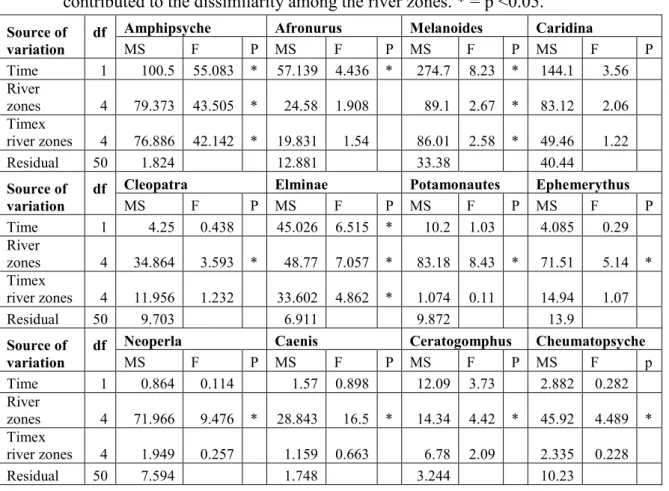
Diversity indices varied significantly among the river zones defined along the Sigi river (ANOVA, Table 4). Time was found to have no influence on the variation of the indices and thus the same pattern was detected in both sampling periods. The post hoc tests showed that the mature rive (MR) zone had significantly less taxa, smaller abundances and smaller values of the indices, relative to the other river zones (Figure 5). Table 4: Results of Analysis of variance (ANOVA) based on biotic indices for the five river zones and two sampling periods (Dry & wet periods). * = p <0.05. Source of variation df No of taxa Total abundances Specis richness (d') Diversity index (H') MS F P MS F P MS F P MS F P Time 1 1.021 0.0623 364.026 0.9 0.017 0.02 0.03 0.22 River zones 4 143.267 8.739 * 1060.097 2.62 * 7.947 10.6 * 2.837 21.1 * Timexriver zones 4 6.942 0.423 307.504 0.76 0.297 0.4 0.114 0.85 Residual 50 16.394 0.749 0.134
Figure 5: Diversity indices (mean± SD) indicating number of taxa, Total number of individuals, Margalef’s species richness index and ShannonWiener diversity index for the dry and wet seasons. MS = Mountains streams, UF = Upper foothill, LF = Lower foothill, REJ = Rejuvenated foothill and MR = Mature lower river. River zones MS UF LF REJ MR Num ber of taxa 0 5 10 15 20 25 Dry season Wet season River zones MS UF LF REJ MR To tal Abu ndanc e 0 20 40 60 80 100 River zones MS UF LF REJ MR M argalef index 0 1 2 3 4 5 6 River zones MS UF LF REJ MR Shannon inde x 0.0 0.5 1.0 1.5 2.0 2.5 3.0
3.2 Macroinvertebrate assemblages
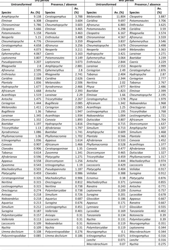
A total of 956 individuals, distributed by 54 taxa, were collected at 9 sites along the river in the dry period. The samples were numerically dominanted by Epherithidae (Epherythus sp.), Potamonautidae (Potamonautes sp.), Hydropsychidae (Hydropsyche sp. & Leptonema sp.) and Thiaridae (Cleopatra sp.), as summarized in Table 5. In the wet period 1280 individuals and 56 taxa of macroinvertebrates were collected in 11 sites along the Sigi river from its headwaters to the low land areas. Actyidae (Caridina sp.), Thiaridae (Melanoides sp. & Cleopatra sp.), Heptageniidae (Afronurus sp.) and Potamonautidae (Potamonautes sp.) were the most abundant taxa (Table 6).
The ANOSIM analyses indicated there were significant differences in the macroinvertebrate assemblages among the five zones defined along the river (Figure 6) in both sampling periods. [(for actual abundance data (Global R =0.8, p<0.05; Global R =0.5, p<0.05 for dry and wet periods respectively) and presence/absence transformed data (Global R =0.8, p<0.05 and Global R =0.5, p<0.05 for dry and wet periods respectively)]. The pairwise tests showed there were significant differences in each pair of the river zones, except in dry period the MR and REJ zones (p=10%) both in terms of taxonomic composition and abundances. The high Global R was observed in this pair (MR and REJ), the lack significant difference which was not expected could be due to lowest number of permutation which was 10. In the wet period the three pairs of river zones MR& REJ, REJ & LF and LF & UF were not significantly different from each other. The remaining pairs were significantly different from each other both in terms of taxa composition and abundances (Table 7).
Taxa contributing to the dissimilarity in macroinvertebrate assemblages among the river zones are tabulated on basis of the overall average contribution to the difference among the river zones. In dry period Amphipsyche, Elminae, Chironominae, Cleopatra and Potamonautes, in wet period Melanoides, Caridina, Afronurus, Potamonautes and Cleopatra are the taxa contributed above 5% for the dissimilarity among the river zones based on their abundances. The greatest contributors to dissimilarities with respect to frequency of occurrence during the dry period were Ceratogomphus, Cleopatra, Cheumatopsyche, Elminae and Plantala; while in the wet season were Cleopatra, Potamonautes, Enthraulus,
Table 5: List of identified taxa (av. abundance ± SD) of macroinvertebrates in the five zones of Sigi river in dry period. Codes; MS Mountain streams, UF Upper foothill, LF Lower foothills, REJ= Rejuvenated foothill, MR Mature river.
Family Genus MS UF LF REJ MR
Total individuals Actyidae Caridina 0.67±1.15 1.67±1.53 7 Athericidae Suragina 0.22±0.45 0.17±0.48 3 Baetidae Acanthiops 0.67±1.32 0.67±1.63 1±1.73 13 Baetidae 1.5±1.38 9 Bugilliesia 1.22±1.32 0.83±0.98 16 Cloeodes 0.22±0.67 1±1.73 5 Pseudopannota 1±2.35 4.17±7.33 34 Xyrodromeus 0.22±0.45 0.33±0.52 1.33±1.53 8 Belastomatidae Appasus 0.33±0.58 0.33±0.58 2 Caenidae Caenis 0.56±0.53 4.33±2.53 1±1.73 34 Calopterygidae Umma declivium 0.22±0.67 2 Ceratopogonidae Ceratopogoninae 0.17±0.48 0.33±0.58 2 Chironomidae Chironominae 1±1.12 1.67±2.88 1.17±1.63 1.33±1.53 4.67±5.69 44 Chlorocyphidae Platycypha 0.33±0.77 0.33±0.52 5 Coenagrionidae Ceriagrion 1.33±1.15 4 Corduliidae Phyllomacromia 1.33±1.21 8 Dicercomyzidae Dicercomyzon 2.33±3.88 0.33±0.58 22 Elmidae Elminae 0.67±0.82 1±1.55 10±11.79 0.67±0.58 42 Larainae 1.22±1.64 0.17±0.48 0.33±0.52 0.67±1.15 16 Ephemerythidae Ephemerythus 7.11±8.90 0.17±0.48 1±1.73 68 Gerridae Aquarius 0.17±0.48 0.17±0.48 2 Naboandelus 0.33±0.82 2 Gomphidae Ceratogomphus 0.44±0.73 2.83±2.32 4.17±4.78 46 Ictinogomphus 1.33±1.75 8 Lestinogomphus 0.33±0.82 2 Gyrinidae Orectogyrus 0.22±0.45 0.17±0.48 3 Heptageniidae Afronurus 2.78±3.32 1.17±0.98 1.33±1.15 36 Hydropsychidae Amphipsyche 0.5±1.22 0.5±1.22 13.67±5.58 47 Cheumatopsyche 4.78±3.87 1.50±1.64 2.67±3.79 0.33±0.58 61 Hydropsyche 0.78±1.56 0.50±0.84 1±1.73 13 Leptonema 5.22±7.12 0.33±0.82 0.17±0.48 0.33±0.58 51 Leptophlebiidae Enthraulus 2.33±2.12 0.67±0.82 0.67±1.21 0.67±0.58 31 Leptopodamorpha Valleriola 0.17±0.48 1 Libellilude Plantala 0.5±0.84 1.67±1.56 0.67±0.58 15 Zyxomma 0.33±0.82 0.33±0.58 3 Machadorythidae Machadorythus 0.33±0.82 0.17±0.48 3 Naucoridae Laccocoris 0.17±0.48 1 Neritidae Neritina 0.67±1.15 2 Notonectidae Anisops 0.33±0.82 2 Nychia 0.17±0.48 1 Perlidae Neoperla 1±1.12 6.67±6.22 49 Polycentropodidae Polycentropodidae 0.11±0.33 1 Polymitarcyidae Polymitarcyidae 0.33±0.58 1 Potamonautidae Potamonautes 5.56±3.57 2.83±3.37 0.17±0.48 68 Prosopistomatidae Africanum 0.67±1.41 1.83±3.26 0.17±0.48 18 Psephenidae larva Afrobrianax 0.33±0.5 0.17±0.48 0.33±0.52 6 Simuliidae Simulium 0.33±0.5 3 Tabanidae Tabanus 0.56±0.73 0.5±0.55 8 Thiaridae Cleopatra 1.33±3.41 1.33±1.97 5.83±3.71 0.67±1.15 57 Melanoides 0.17±0.48 0.67±0.82 1.67±1.53 10 Tipulidae Antocha 0.5±0.55 2.33±3.21 10 Conosia 1±0.87 0.5±1.22 12 Tricorythidae Tricorythidae 0.11±0.33 0.17±0.48 1.67±1.53 7 Veliidae Rhagovelia 2.11±2.571 1.33±1.97 0.17±0.48 1.33±2.39 32 Total abundances 414 213 157 144 28 956 No of Taxa 31 33 27 26 7 54 Shannon index (H) 2.22 3.19 1.96 2.07 1.04 Margalef index (d) 3.27 3.19 2.75 3.05 1.24 No of samples 9 6 6 3 3
Table 6: List of identified taxa (av. abundance ± SD) of macroinvertebrates in the five zones of Sigi river in wet period. Codes; MS Mountain streams, UF Upper foothill, LF Lower foothills, REJ= Rejuvenated foothill, MR Mature river.
Family Genus MS UF LF REJ MR
Total individuals Actyidae Caridina 8.5±1.31 12.4±18.47 113 Athericidae Suragina 0.22±0.45 0.17±0.48 3 Baetidae Acanthiops 1.89±3.14 0.33±0.82 19 Baetidae 1.33±2.69 1.17±0.98 0.67±1.21 0.33±0.52 25 Glossidon 0.33±0.77 3 Tanzaniela 0.17±0.48 1 Belastomatidae Appasus 0.33±0.52 2 Caenidae Caenis 0.5±0.84 3.17±2.93 0.5±0.55 25 Chironomidae Chironominae 1±1 1±1.26 0.67±0.82 4.5±5.55 0.2±0.45 47 Chlorocyphidae Platycypha 0.33±0.82 0.17±0.48 3 Coenagrionidae Ceriagrion 0.89±2.28 3.17±4.26 0.83±1.17 32 Corduliidae Phyllomacromia 0.11±0.33 0.17±0.48 0.33±0.82 0.33±0.82 6 Dicercomyzidae Dicercomyzon 0.44±0.53 0.17±0.48 0.17±0.48 6 Dytiscidae Dytiscidae 0.22±0.67 1.17±1.83 0.17±0.48 10 Economidae Ecnomus 0.33±0.82 0.17±0.48 3 Elmidae Elminae 0.11±0.33 1.67±1.56 1.33±2.85 19 Larainae 1.44±2.30 2.17±2.14 1.17±1.47 0.33±0.52 35 Ephemerythidae Ephemerythus 3.33±2.40 1.33±1.75 0.67±1.33 0.2±0.45 43 Gerridae Naboandelus 0.33±0.52 0.33±0.52 0.6±1.34 7 Gomphidae Ceratogomphus 0.33±0.77 0.83±0.98 1±1.26 0.5±0.84 17 Ictinogomphus 0.17±0.48 1 Lestinogomphus 1.67±2.58 0.17±0.48 0.2±0.45 12 Neurogomphus 0.17±0.48 1 Gyrinidae Orectogyrus 0.89±1.55 0.17±0.48 0.17±0.48 10 Heptageniidae Afronurus 4.67±5.5 1.67±2.66 6.67±7.28 2.5±2.59 0.2±0.45 108 Hirunidea Leeche 0.17±0.48 1 Hydropsychidae Amphipsyche 0.56±1.33 0.33±0.52 7 Cheumatopsyche 4.11±5.78 2.17±3.71 0.67±1.63 54 Hydropsyche 3.89±6.92 1±1.26 1.17±2.41 48 Leptonema 0.5±1.22 3 Leptophlebiidae Enthraulus 1.89±1.27 0.67±1.21 2±2.98 1.83±4.5 44 Libellilude Plantala 0.67±0.82 0.17±0.48 5 Lycosidae Lycosidae 0.22±0.45 2 Lymnaeidae Lymnaea 0.17±0.48 0.2±0.45 2 Machadorythidae Machadorythus 0.5±0.84 3 Naucoridae Laccocoris 0.22±0.67 0.5±0.84 5 Nepidae Ranatra 0.5±0.84 3 Neritidae Neritina 0.5±0.55 3.6±4.98 21 Notonectidae Notonecta 0.17±0.48 1 Nychia 0.22±0.67 2 Palaemonidae Macrobrachium 0.17±0.48 1 Perlidae Neoperla 1.22±1.72 5±5.51 0.17±0.48 42 Physidae Physa 0.11±0.33 2.67±3.33 0.17±0.48 0.17±0.48 19 Polymitarcyidae Polymitarcyidae 0.17±0.48 1 Potamonautidae Potamonautes 6.11±4.26 4.5±5.32 1±2 1.6±2.6 96 Prosopistomatidae Africanum 1.22±1.72 1±2 17 Psephenidae larva Afrobrianax 0.44±1.14 0.33±0.52 6 Simuliidae Simulium 0.89±1.54 0.33±0.52 10 Tabanidae Tabanus 2±2.65 1.67±2.34 0.5±1.22 0.33±0.82 33 Thiaridae Cleopatra 1.33±2.18 4.5±6.83 3.67±1.86 2.5±2.6 76 Melanoides 0.11±0.33 2.83±3.13 1±1.95 6.5±7.45 17.8±16.34 152 Tipulidae Antocha 0.67±1.33 4 Conosia 0.11±0.33 0.5±0.84 0.17±0.48 5 Tricorythidae Tricorythidae 0.17±0.48 0.17±0.48 0.33±0.52 4 Veliidae Rhagovelia 2.11±1.45 0.83±2.41 2.5±3.17 3±3.69 57 Veliidae 0.22±0.67 0.33±0.82 0.17±0.48 5
Figure 6: MDS ordination showing the spatial distribution of macroinvertebrate assemblages along Sigi River in dry and wet periods. a & b MDS generated from untransformed data for dry and wet periods respectively, c & d MDS from Presence/absence transformation for the dry and wet periods respectively. Codes; MS =Mountains streams, UF = Upper foothills, LF = Lower foothills, REJ = Rejuvenated foothills, MR =Mature river.
Table 7: Analysis of Similarity (ANOSIM) among river zones and between the sampling period (dry and wet periods). Significant, as determined by pairwise test, are indicated with *= p<0.05, NS =Not significant; MS = Mountains streams, UF = Upper foothill, LF = Lower foothill, REJ = Rejuvenated foothill and MR = Mature lower river. River zones Dry period Wet period Untransformed Presence/ Absence Untransformed Presence/ Absence Global R p Global R p Global R p Global R p
MS, MR 0.985 * 0.996 * 0.952 * 0.928 * MS, REJ 0.78 * 0.782 * 0.682 * 0.649 * MS, LF 0.962 * 0.968 * 0.326 * 0.382 * MS, UF 0.34 * 0.493 * 0.257 * 0.345 * MR, REJ 0.852 NS 0.593 NS 0.263 NS 0.436 * MR, LF 0.975 * 0.991 * 0.884 * 0.884 * MR, UF 0.79 * 0.907 * 0.787 * 0.904 * REJ, LF 0.963 * 0.809 * 0.094 * 0.016 NS REJ, UF 0.698 * 0.438 * 0.292 * 0.404 * LF, UF 0.759 * 0.794 * 0.261 NS 0.251 NS