F
ACULDADE DEE
NGENHARIA DAU
NIVERSIDADE DOP
ORTOA Scalable, Self-organizing
Communications System for very large
Wireless Sensor Networks
Mohammad Mahmoud Abdellatif
Programa Doutoral em Telecomunicações
Orientador: Doutor José Manuel Soares Oliveira, da Faculdade de Economia da Universidade do Porto
Co-Orientador: Doutor Manuel Alberto Pereira Ricardo, do Departamento de Engenharia Eletrotécnica e de Computadores da Faculdade de Engenharia da
Universidade do Porto
c
A Scalable, Self-organizing Communications System for
very large Wireless Sensor Networks
Mohammad Mahmoud Abdellatif
Programa Doutoral em Telecomunicações
Aprovado em provas públicas pelo Júri:
Presidente: Doutor José Alfredo Ribeiro da Silva Matos, Professor Catedrático da Facul-dade de Engenharia da UniversiFacul-dade do Porto
Arguente: Doutor Jorge Sá Silva, Professor Auxiliar do Departamento de Engenharia Informática da Faculdade de Ciências e Tecnologia da Universidade de Coimbra
Arguente: Doutor Joel José Puga Coelho Rodrigues, Professor Auxiliar do Departamento de Informática da Universidade da Beira Interior
Vogal: Doutor Adriano Jorge Cardoso Moreira, Professor Associado do Departamento de Sistemas de Informação da Escola de Engenharia da Universidade do Minho
Vogal: Doutor Vítor Manuel Grade Tavares, Professor Auxiliar do Departamento de En-genharia Eletrotécnica e de Computadores da Faculdade de EnEn-genharia da Universidade do Porto
Vogal: Doutor José Manuel Soares Oliveira, Professor Auxiliar da Faculdade de Econo-mia da Universidade do Porto (Orientador)
The best way out is always through.
Robert Frost.
Acknowledgments
First and foremost I would like to thank Allah for His kindest blessings on me and all the members of my family. And for always helping me find the right path even when I felt that there is none.
My deep appreciation goes to my advisor Prof. José Manuel Oliveira. He was always there when I needed him ever since the day I arrived to Porto. I am extremely grateful to him for his prompt replies to my questions and his numerous proofreads of all the work that was done during the Phd. I am thankful to his help and support inside and outside the work.
I would like also to thank my other advisor Prof. Manuel Ricardo. I appreciate all his contributions of time, ideas, even with his busy schedule, he could always find the time to discuss the work and give me his feedback which has always resulted in the improvement of the work.
The help and support of my research institute INESC TEC can not go without notice. It has been a privilege to work in this environment that is dedicated to research and to help young researchers achieve their potential. I had many discussions with my colleagues here that helped me improve my work and I am really thankful to all their help and friendship. I like to thank: Bruno Marques, Dossa Massa, Helder Fontes, Jaime Dias, Muhammad Ajmal, Nuno Salta (“RIP”), Pedro Fortuna, Pedro Pinto, Pedro Silva, Renata Rodrigues, Rui Campos, Saravanan Kandasamy. Apologies to anyone I forgot.
Thanks to Faculdade de Engenharia da Universidade do Porto for providing excellent education and accepting me as student. It is truly one of the best faculties that I had the privilege to study in. This work is funded by the ERDF through the Program COMPETE and by the Portuguese Government through FCT-Fundação para a Ciência e Tecnologia, project ref. CMU- PT / SIA / 0005 / 2009 and by the research grant number SFRH / BD /
iv
68759 / 2010.
I can not forget to thank my friend and neighbor Hazem Ali for his support and friend-ship during my years here in Portugal. Many things would have gone badly in my life if it weren’t for his help. I would also like to thank Rita Pacheco for her help with the abstract translation.
Last but not least, I humbly offer my sincere thanks to my parents for their incessant inspiration, blessings and prayers. They never gave up on me and they always pushed me forward. I don’t think I would have been able to finish if it weren’t for their support and for that I am eternally grateful.
Resumo
As redes de sensores sem fios (Wireless Sensor Networks, WSNs) são formadas por uma grande quantidade de nós de dimensões reduzidas que são capazes de detetar mudanças num ambiente e comunicá-las através da rede. Um exemplo deste tipo de rede é uma central fotovoltaica (FV), onde existe um sensor ligado a cada painel solar. Cada sensor é responsável por detetar a produção do painel, que é depois enviada para um nó central para ser processada.
Apesar das redes de sensores sem fios transmitirem dados em baixo débito, estas ap-resentam ainda outros desafios que estão maioritariamente ligados à eficiência das comu-nicações e à eficiência energética. Além disso, à medida que a rede cresce, torna-se im-praticável ou mesmo impossível configurar todos estes nós manualmente. Portanto, neste contexto é essencial usar algoritmos de auto-organização e configuração. Mais ainda, dev-ido à caraterística “muitos para um” (many-to-one) da comunicação nas redes de sensores sem fios, assim como as interferências ecolisões, a recolha programada de dados torna-se um grande desafio que deve ser cuidadosamente analisado.
Este trabalho aborda dois problemas: a autoconfiguração de nós e a recolha de da-dos a partir desses nós. Para o problema da autoconfiguração de nós são propostos três algoritmos que permitem aos nós da rede identificar automaticamente os seus vizinhos mais próximos, a sua posição relativa na rede, e selecionar o canal de frequência em que devem operar. Para isso, é utilizado o valor da indicação do nível de sinal recebido (Re-ceived Signal Strength Indicator, RSSI) das mensagens enviadas e recebidas durante a fase de configuração. O desempenho destes algoritmos é testado através de simulações e testbeds. Foi possível concluir que os algoritmos permitem que os nós se autoconfigurem sem qualquer interferência do operador da rede. Os resultados demonstram que o erro ao nível do desempenho decresce à medida que se aumenta o número dos valores de RSSI
vi
utilizados para a tomada de decisões. Além disso, o número de nós na rede afeta consid-eravelmente o erro de configuração. No entanto, o valor do erro é ainda aceitável mesmo para um grande número de nós simulados.
Relativamente ao problema da recolha de dados, foi avaliado o desempenho de três técnicas diferentes de recolha, com e sem agregação de dados. Este estudo considerou uma rede sem fios com um número fixo de nós, utilizando diferentes valores de tráfego oferecido, tendo sido possível estimar a capacidade de transmissão da rede para cada técnica, assim como para cada valor de tráfego oferecido.
Abstract
Wireless Sensor Networks (WSNs) are made of a large amount of small devices that are able to sense changes in the environment and communicate these changes throughout the network. An example of such network is a photo voltaic (PV) power plant, where there is a sensor connected to each solar panel. The task of each sensor is to sense the output of the panel which is then sent to a central node for processing. Even though low data rate is employed in WSNs, other challenging issues appear in the network.
Challenges are mostly related to the reliability of the communication links and to the energy efficiency. Moreover, as the network grows, it becomes impractical and even impossible to configure all these nodes manually. The use of self-organization and auto-configuration algorithms becomes essential in this context. Also, because of the “many-to-one” feature of the communication in WSNs, the wireless interferences and the colli-sions, the scheduling of data collection becomes a challenging problem which needs to be carefully addressed.
This work addresses these two problems: the self-configuration of nodes and the data collection from nodes. For the self-configuration problem, three algorithms are proposed that allow nodes in the network to automatically identify their closest neighbors, their relative location in the network, and select which frequency channel to operate in. This is done using the value of the Received Signal Strength Indicator (RSSI) of the messages sent and received during the setup phase. The performance of these algorithms is tested by means of both simulations and testbed experiments. We were able to conclude that the algorithms allow nodes to configure themselves with no interference from the operator of the network. Results showed that the error in performance decreases as we increase the number of RSSI values used for decision making. Additionally, the number of nodes in the network affects the setup error greatly. However, the value of the error is still
viii
acceptable even for high number of simulated nodes.
As for the data collection problem, we have evaluated the performance of three differ-ent data collecting techniques with and without data aggregation. The study considered a wireless network with fixed number of nodes using different values of the offered load, estimating the network throughput for each technique and offered load.
Contents
1 Introduction 1
1.1 Motivation . . . 1
1.2 Problem Statement . . . 2
1.3 Objectives . . . 2
1.4 Overview of the Proposed Network Topology . . . 3
1.5 Main Contributions . . . 4
1.5.1 Self-Configuration of Nodes . . . 4
1.5.2 Aggregated Data Collection Technique . . . 5
1.6 Overview of Published and Submitted Papers . . . 6
1.7 Structure of the Thesis . . . 6
2 Background and Related Work 9 2.1 Background . . . 9
2.1.1 The Internet Protocol Suite . . . 9
2.1.2 IEEE 802.3 . . . 11
2.1.3 IEEE 802.15.4 . . . 13
2.1.3.1 Topologies . . . 13
2.1.3.2 Physical Layer . . . 14
2.1.3.3 Medium Access Control (MAC) . . . 14
2.1.4 Internet Protocol . . . 16
2.1.4.1 IPv4 . . . 17
2.1.4.2 IPv6 . . . 19
2.1.5 The Internet of Things . . . 21
2.1.6 6LoWPAN . . . 22
x CONTENTS
2.1.6.1 Motivations . . . 23
2.1.6.2 Packet Compression . . . 23
2.1.6.3 Fragmentation . . . 25
2.1.7 Contiki Operating System . . . 26
2.1.8 TinyOS . . . 28
2.1.9 COOJA . . . 28
2.1.10 TelosB Sky Motes . . . 30
2.2 Related Work . . . 33
2.2.1 Self-Configuration . . . 33
2.2.2 Data Collection . . . 36
3 Self-Configuration 41 3.1 Proposed Topology and Self-Configuration Algorithms . . . 43
3.1.1 Network Topology . . . 43
3.1.2 Neighbor Identification Algorithm . . . 44
3.1.3 Relative Location Algorithm . . . 47
3.1.4 Frequency Allocation Algorithm . . . 50
3.2 Simulation Environment . . . 52
3.3 Simulation Results and Analysis . . . 53
3.3.1 Neighbor Identification Algorithm . . . 54
3.3.2 Relative Location Algorithm . . . 54
3.3.3 Frequency Allocation Algorithm . . . 55
3.4 Testbed Experiments and Results . . . 56
3.4.1 Indoor Experiment . . . 56
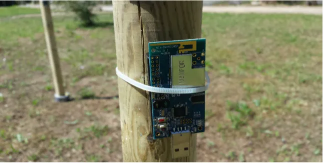
3.4.2 Panels Experiment . . . 58
3.4.3 Outdoor Experiment . . . 61
3.5 Conclusions . . . 66
4 Data Collection 67 4.1 Proposed Architecture and Data Collection Techniques . . . 69
4.2 Simulation and Testbed Environments . . . 72
CONTENTS xi
4.3.1 Link Analysis . . . 73
4.3.2 Performance of the Techniques . . . 74
4.3.3 Performance of the Modified Techniques with no Sink Command Messages . . . 81
4.3.4 Performance of the Modified Techniques with Sink Command Messages enabled . . . 82
4.3.5 Packet Loss Per Node of the Techniques with no Sink Command Messages . . . 83
4.3.6 Testbed Experiments . . . 85
4.4 Conclusions . . . 86
5 Conclusions 89 5.1 Overview of the Work . . . 89
5.2 Summary of Contributions . . . 91
5.2.1 Self-Configuration of Nodes . . . 91
5.2.2 Aggregated Data Collection Technique . . . 92
5.3 Future Research . . . 93
List of Figures
1.1 Network topology. . . 4
2.1 The TCP/IP stack. . . 10
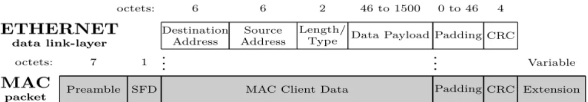
2.2 Ethernet data link layer protocol encapsulated into the MAC Client Data field of a IEEE 802.3 MAC packet. . . 12
2.3 IEEE 802.15.4 data frame. . . 15
2.4 IPv4 datagram header. . . 17
2.5 IPv6 datagram header. . . 20
2.6 6LoWPAN intermediate layer. . . 22
2.7 6LoWPN IPHC base header. . . 24
2.8 The architecture of Contiki. . . 27
2.9 Tmote Sky front. . . 31
2.10 Tmote Sky back. . . 31
3.1 Network topology. . . 44
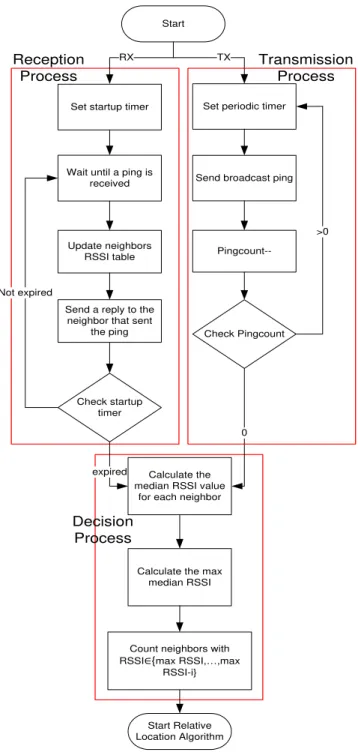
3.2 Neighbor identification algorithm. . . 45
3.3 Relative location algorithm. . . 48
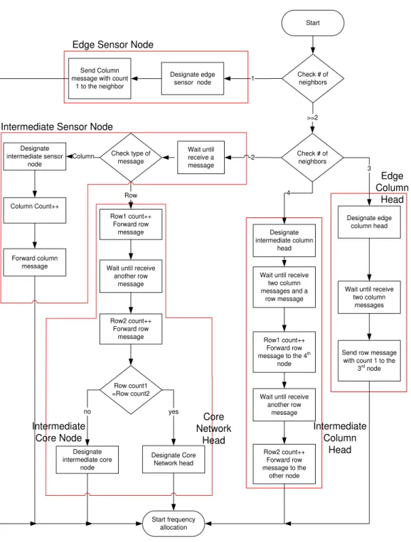
3.4 Frequency allocation algorithm. . . 50
3.5 Indoor Experiment (a) 3-mote network. (b) 4-mote network. . . 56
3.6 Indoor Experiment 4-mote network. . . 57
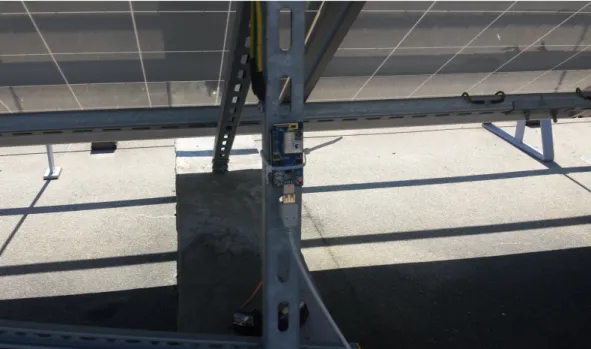
3.7 Panels Experiment. . . 58
3.8 Panels Experiment (one node). . . 59
3.9 Panels Experiment (1st column). . . 59
3.10 Panels Experiment (2nd column). . . 60
3.11 Outdoor Experiment. . . 62
xiv LIST OF FIGURES
3.12 Outdoor Experiment (all nodes). . . 62
3.13 Outdoor Experiment (one node). . . 63
4.1 Network topology. . . 69
4.2 Proposed data collection and communication techniques. . . 70
4.3 Modified data collection and communication techniques. . . 71
4.4 Throughput vs. offered load for a system with one client node. . . 74
4.5 Average throughput for an offered load of 1 packet/s/node. . . 75
4.6 Average throughput for an offered load of 2 packet/s/node. . . 75
4.7 Average throughput for an offered load of 4 packet/s/node. . . 76
4.8 Total packet loss for an offered load of 1 packet/s/node. . . 76
4.9 Total packet loss for an offered load of 2 packet/s/node. . . 77
4.10 Total packet loss for an offered load of 4 packet/s/node. . . 77
4.11 Total delay for an offered load of 1 packet/s/node. . . 78
4.12 Total delay for an offered load of 2 packet/s/node. . . 78
4.13 Total delay for an offered load of 4 packet/s/node. . . 78
4.14 Node packet loss of a network with 8 client nodes for different values of offered load. . . 80
4.15 Throughput vs. offered load for an 8 clients network for the modified techniques with no sink command messages. . . 81
4.16 Throughput vs. offered load for an 8 clients network for the modified techniques with sink command messages enabled. . . 82
4.17 Command message throughput vs. offered load for an 8 clients network for the modified techniques with sink command messages enabled. . . 83
4.18 Packet loss per node for an offered load of 6 packet/s/node. . . 84
4.19 Packet loss per node for an offered load of 7 packet/s/node. . . 84
4.20 Packet loss per node for an offered load of 8 packet/s/node. . . 84
List of Tables
2.1 IEEE 802.15.4 physical layers . . . 14
2.2 Advanticsys MTM-CM5000-MSP general specifications. . . 32
3.1 Error performance of the Neighbor Identification Algorithm. . . 54
3.2 Error performance of the Relative Location Algorithm. . . 55
3.3 Error performance of the Frequency Allocation Algorithm. . . 55
3.4 Median RSSI in dBm per node in a 3-mote indoor network. . . 57
3.5 Median RSSI in dBm per node in a 4-mote indoor network. . . 58
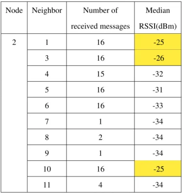
3.6 Median RSSI in dBm per neighbor for a node with one close neighbor. . . 60
3.7 Median RSSI in dBm per neighbor for a node with two close neighbors. . 61
3.8 Median RSSI in dBm per neighbor for a node with three close neighbors. 61 3.9 Median RSSI in dBm per neighbor for a node with one close neighbor. . . 63
3.10 Median RSSI in dBm per neighbor for a node with two close neighbors. . 64
3.11 Median RSSI in dBm per neighbor for a node with three close neighbors. 64 3.12 Median RSSI in dBm per neighbor for a node with four close neighbors. . 65
3.13 Error performance of the algorithms in the testbed experiments. . . 65
Abbreviations
6LoWPAN IPv6 over Low Power Wireless Personal Network AMA Advanced Metering Infrastructure
AWGN Additive White Gaussian Noise CoAP Constrained Application Protocol
CSMA/CA Carrier Sense Multiple Access with Collision Avoidance CSMA/CD Carrier Sense Multiple Access with Collision Detection CRC Cyclic Redundancy Check
DAG Directed Acyclic Graph
DAO Destination Advertisement Object DIO DODAG Information Object
DODAG Destination-Oriented Directed Acyclic Graph DSSS Direct Sequence Spread Spectrum
ETX Expected Transmission Count FFD Full Function Device
FHSS Frequency Hopping Spread Spectrum GTS Guaranteed Time Slot
HTTP Hypertext Transfer Protocol ICMP Internet Control Message Protocol
IEEE Institute of Electrical and Electronics Engineers IETF Internet Engineering Task Force
IFS Inter-Frame Space
INESC Instituto de Engenharia de Sistemas e Computadores IP Internet Protocol
IPHC Internet Protocol Header Compression
xviii Abbreviations
LLN Low Power, Lossy Network LQI Link Quality Indicator
LR-WPAN Low Rate Wireless Personal Area Networks MAC Medium Access Control
MPDU MAC Protocol Data Unit MRM Multi-path Ray-tracer Medium MTU Maximum Transfer Unit
OFDM Orthogonal Frequency Division Multiplexing OSI Open Systems Interconnection
PAN Personal Area Network PCF Point Coordination Function PHY Physical Layer
PV Photo Voltaic
RFC Request for Comments RFD Reduced Function Device RFID Radio Frequency Identification
RPL Routing Protocol for Low Power Lossy Networks RSSI Received Signal Strength Indicator
SICS Swedish Institute of Computer Science
SELF-PVP Self-organizing power management for photo-voltaic power plants TCP Transmission Control Protocol
UDP User Datagram Protocol UDGM Unit Disk Graph Medium
Chapter 1
Introduction
Wireless Sensor Networks (WSNs) have been a hot research topic in the recent years. They consist of a large amount of small devices that are able to sense changes in the envi-ronment and communicate these changes throughout the network [1]. WSN applications are various, they are used in smart-cities, environmental monitoring, distributed sensing in industrial plants, and health care [2].
Even though low data rate is employed in WSNs, other challenging issues appear in the network. Challenges are mostly related to the reliability of the communication links and to the energy efficiency [3]. Also, because of the “many-to-one” feature of the communication in WSNs, the wireless interferences and the collisions, the scheduling of data collection becomes a challenging problem which needs to be carefully addressed.
1.1
Motivation
The need for an alternative and clean power source has grown continuously over the past years since the world is still mostly dependent on the use of fossil fuel which has a lot of negative effects on the environment. One of the main sources of alternative energy is solar power, which has proven to be a good choice to replace fossil fuel. However, even with the current technology, and with a large solar power plant, the efficiency of the power generation is not sufficient. An example of a photo-voltaic (PV) power plant is the
2 Introduction
Almaraleja power plant, in Alentejo, Portugal, in which the number of solar panels could go above 200,000 spread over a large area (250 hectares).
The main motivation that drives this PhD research is to achieve an increase in power efficiency in photo-voltaic power plants. The increase will be achieved using a novel, distributed, real time adaptive network controller of sensors/actuators, where a sensor node is connected to each solar panel in the network, to bring optimality to the overall power output of the panels’ array. The small and low power wireless sensor nodes will sense local variables, communicate among each other these variables and compute local errors with the goal of optimizing, in real time, the overall performance of the panels’ array. Our work is focused on allowing those many sensors nodes to communicate with each others reliably in order to achieve this goal.
1.2
Problem Statement
The first problem that arises is that as this communications network grows, it becomes impractical or even impossible to configure all the nodes in the network manually. In order to solve this problem, the use of self-organization and auto-configuration algorithms becomes essential.
Secondly, the interference among the nodes and the large set of neighboring nodes will increase as the number of nodes continue to increase. Interference will increase the rate of frame retransmissions. and to reduce the reliability of the network.
Furthermore, sensor data has to be collected from nodes in a way that is reliable re-gardless of the topology of the network which can be very dense with a very high number of nodes.
1.3
Objectives
1.4 Overview of the Proposed Network Topology 3
The goal is to add self-organization and scalability to a distributed communication network, with the ability to sense and control the operation of a dense wireless sensor network.
Due to the specificity of the sensor network (heterogeneous data, real time constraints, several communication modes - broadcast and unicast, grid topology) a dedicated wireless system design will have to be undertaken. Although the research here presented has a key application in mind - the power optimization in PV power plants - we envision many other applications - tackling generic global optimization with sensor networks.
This PhD focuses on solving the problem of the self-organization of sensors in clus-ters, which also includes their auto-configuration and frequency planning. Additionally, we tackle the efficient broadcast based data collection and communications in a large net-work. Using simple communications techniques for the transmission and routing of data, while preserving some degree of reliability.
1.4
Overview of the Proposed Network Topology
The proposed WSN topology is shown in Figure1.1. Such setup is referred to as a strip-based deployment and it allows for full coverage of the area under consideration. In a real life scenario, the nodes within a column are placed side by side with a distance of about 2 meters between each consecutive sensor, while columns have a more wider distance between them in order to allow maintenance access.
4 Introduction
Column Head
Core Network Node Sensor Node Core Network
Head
Fc
F1 F2 F3 F4 F5
Fx
Frequency Channel
Figure 1.1: Network topology.
1.5
Main Contributions
This PhD thesis has two main contributions, which are described in the following subsec-tions.
1.5.1 Self-Configuration of Nodes
Three novel algorithms were proposed that, when run consecutively, allow each node in the system to identify its neighbors, locate its relative location in the network, and select its operating frequency channel in order to reduce the overall interference among nodes.
These algorithms were designed for this specific network where nodes are placed in a static grid topology and where nodes communicate mainly with their neighbors within the same column. There are related algorithms proposed in the literature [4,5]. However, none of them meet the needs of the objectives mentioned above.
1.5 Main Contributions 5
nodes in the network after booting. Using this information, nodes calculate which neighbor(s) has the highest RSSI value. These neighbors will be considered then as the closest neighbors in the network. Nodes are required to know their closest neighbors in the network in order to limit the communication between these nodes and so, reduce any unwanted traffic and in turn leads to less interference, and less energy consumption, which will lead to the ability of adding more nodes to the network.
• Relative Location Algorithm. Used to enable each node to find its relative loca-tion in the network with respect to the other nodes and decide its role in the network based on that location. The role of each node will dictate how will it behave through-out its lifetime. The node’s role is determined with no interference from the network operator with all the nodes having the same code and the same hardware.
• Frequency Allocation Algorithm. This algorithm is used to divide the network into small networks of columns where every column operate in a different frequency channel. The allocation is done in order to reduce the interference among the nodes as well as to enable the scalability of the solution. The core network will be still operating in the initial frequency in order to allow nodes in different columns to communicate with each others if needed.
These three novel algorithms allow the complete and automatic self-configuration of nodes in a static network with grid topology with no interference from the network oper-ator. No other solution was found in literature that was able to achieve these goals for the specific network proposed in this work.
1.5.2 Aggregated Data Collection Technique
6 Introduction
Using the proposed polling technique to collect data from the nodes increases the end to end delay, however, as the rate of change in the state of the network is slow, this level of delay can be considered as acceptable. The proposed technique was compared with other existing techniques in literature and was proven, in the specific network we are testing, to further reduce the traffic being sent back and forth between the nodes, and increases the reliability of the network.
1.6
Overview of Published and Submitted Papers
• Published a conference paper entitled “Impact of Data Collecting Techniques on the Performance of a Wireless Sensor Network", in Proceedings of the ISWCS 2012, the Ninth International Symposium on Wireless Communication Systems, Paris, France, August 28-31 [6].
• Published a conference paper entitled “The Effect of Data Aggregation on the Performance of a Wireless Sensor Network Employing a Polling Based Data Collecting Technique", to the Wireless Days 2013 conference WD’13, Valência, Spain, November 13-15 [7].
• Published a conference paper entitled “Neighbors and Relative Location Identi-fication Using RSSI in a Dense Wireless Sensor Network", to the 13th Annual Mediterranean Ad Hoc Networking Workshop, Piran, Slovenia, June 2-4, 2014 [8].
• Submitted a journal paper entitled “The Self-Configuration of Nodes Using RSSI in a Dense Wireless Sensor Network to the Telecommunication Systems journal. Submitted on the 15th of October 2014. Currently under review.
1.7
Structure of the Thesis
1.7 Structure of the Thesis 7
Chapter 2
Background and Related Work
In this chapter, we give a brief summary of the technologies that we are using in the scope of this thesis and we list some of the related work that could be found in the literature.
2.1
Background
In this section, we discuss in details some of the protocols and technologies that we used to achieve the goals of this thesis. Some of these protocols include the Internet protocol suite and the different stack protocols used. We also discuss the operating system, the simulation environment as well as the hardware platform that we used to carry on the analysis and simulation of the proposed algorithms.
2.1.1 The Internet Protocol Suite
The Internet Protocol Suite is a set of communication protocols grouped for the first time in RFC 1122 [9] and RFC 1123 [10]. It is also known as TCP/IP protocol stack due to the division into abstraction layers of the communications suite. The information flows in both directions, but each layer communicates only with the layer immediately above or beneath. This is done by encapsulating the data on the way down and de-encapsulating it on the way up. In order for this communication to happen, each layer requires the layer underneath to meet certain requirements. At the same time, each layer should fulfill the requirements of the layer immediately above.
10 Background and Related Work
The Internet Protocol Suite is divided into four abstraction layers according to RFC 1122: Link Layer, Internet Layer, Transport Layer, and Application Layer. However, due to the usual mapping of the TCP/IP stack onto the International Standards Organization’s Open System Interconnect (OSI) model, it is also common to refer to the Physical Layer as a hardware layer at the lowest part of the Link Layer. Figure2.1, illustrates the TCP/IP protocol stack, including the Physical Layer within its lowest level.
Application Layer
Transport Layer
Internet Layer
Link Layer
Physical Layer
Figure 2.1: The TCP/IP stack.
Link Layer Groups the different protocols that operate only between adjacent nodes in the same link segment.
Internet Layer Is the set of protocols in charge of delivering packets from the originating host to the destination, traversing different networks if necessary. Due to the mapping onto the OSI model, it is also commonly referred to as “Network Layer”.
2.1 Background 11
Application Layer The set of protocols involved in the process-to-process communi-cation.
2.1.2 IEEE 802.3
12 Background and Related Work
octets: 6 6 2 46 to 1500 0 to 46 4 ETHERNET
data link-layer
Destination Address
Source Address
Length/
Type Data Payload Padding CRC
octets: 7 1 ... ... Variable
MAC
packet Preamble SFD MAC Client Data Padding CRC Extension
Figure 2.2: Ethernet data link layer protocol encapsulated into the MAC Client Data field of a IEEE 802.3 MAC packet.
Preamble Used for synchronization between the sender and the receiver.
SFD Start of Frame Delimiter. Indicates the end of the preamble and the start of the packet data. It has a constant value of 0xAB.
Destination Address 48-bit IEEE 802.3 MAC address of the destination of the frame.
Source Address 48-bit IEEE 802.3 MAC address of the originator of the frame.
Length/Type This field can have two different meanings. If its value is greater than 1500, then it indicates the type of the upper-layer packet be-ing transported. If the field value is less than or equal to 1500, it indicates the length of the payload.
Data Payload The data being transmitted.
Padding Optional Padding. This field is required if the total Ethernet frame length is less than 64 bytes.
CRC Cyclic Redundancy Check for integrity verification.
2.1 Background 13
2.1.3 IEEE 802.15.4
The IEEE 802.15.4 standard [12] specifies the physical and media access control (MAC) for low-rate wireless personal area networks (LR-WPANs). Although LR-WPANs fall within the wireless personal area networks (WPANs) family of standards, they may ex-tend the personal operating space. An LR-WPAN is a simple, low-cost wireless commu-nication network optimized for use in applications with limited power and low throughput requirements.
LR-WPANs main aims are low power consumption and low cost, while maintaining a reliable data transfer, short-range communication link, and simple, flexible protocol.
2.1.3.1 Topologies
The IEEE 802.15.4 standard defines two different device types: full-function devices (FFDs) and reduced-function devices (RFDs). FFDs can participate in the Personal Area Network (PAN) as a PAN coordinator, a coordinator, or as a normal device. Even though a network may consist of just RFDs, the presence of at least one FFD acting as a PAN coordinator is recommended.
14 Background and Related Work
2.1.3.2 Physical Layer
Since its release in 2003, different amendments have been defined adding new possible physical layers and/or extending the capabilities of the previously defined ones. The main different unlicensed frequency bands and modulations, together with the supported data rates defined by the IEEE 802.15.4 physical layer are shown in Table2.1.
Table 2.1: IEEE 802.15.4 physical layers
Physical Frequency
Layer Band Modulation Bit rate
(MHz) (MHz) (kb/s)
868/915 868 - 868.6 BPSK 20
902 - 928 40
868/915 868 - 868.6 ASK 250
902 - 928 250
868/915 868 - 868.6 O-QPSK 100
902 - 928 250
2450 2400 - 2483.5 O-QPSK 250
250 - 750 851,110,
UWB 3244 - 4742 BPM-BPSK 6810, and
5944 - 10234 27240
2450 (CSS) 2400 - 2483.5 DQPSK 250, 1000
780 779 - 787 O-QPSK 250
780 779 - 787 MPSK 250
950 950 - 956 GFSK 100
950 950 - 956 BPSK 20
2.1.3.3 Medium Access Control (MAC)
The IEEE 802.15.4 MAC layer is responsible for the following tasks:
2.1 Background 15
• PAN association and disassociation;
• Employing the CSMA-CA mechanism for channel access;
• Handling and maintaining the Guaranteed Time Slot (GTS) mechanism;
• Frame validation;
• Acknowledged frame delivery;
• Supporting device security.
In star-topologies, the IEEE 802.15.4 MAC layer provides a beacon-based synchroniza-tion mechanism for data transmission and recepsynchroniza-tion between devices and the PAN coor-dinator, which permits nodes to only listen to the channel at regular intervals, allowing for power saving. In peer-to-peer topologies, however, this synchronization mechanism is not provided by the standard and, if required by specific applications, it needs to be implement at upper layers.
The MAC layer defines four different types of frames: beacon frames, acknowledg-ment frames, MAC command frames, and data frames. Beacon frames are used in the synchronization mechanism. Acknowledgment frames, whose use is optional, are used to acknowledge transmissions. MAC command frames carry protocol commands, such as “Association request”, or “Data request”. Finally, data frames are used for all transfers of data. Figure2.3 illustrates the structure of a data frame. The fields of that frame are explained in more details next.
octets: 2 1 4 to 20 n 2
MAC
layer FCF
Sequence
Number Addressing fields Data Payload FCS
octets: 4 1 1 ... 9 to 127 ...
PHY
layer
Preamble Sequence SFD
Frame
Length MPDU
Figure 2.3: IEEE 802.15.4 data frame.
16 Background and Related Work
SFD Start of Frame Delimiter. Indicates the end of the preamble and the start of the packet data. It has constant value of 0xE5.
Frame Length Length of the MAC protocol data unit (MPDU).
FCF Frame Control Field. Contains information defining the frame type, addressing modes, and other control flags.
Sequence Number Used to match acknowledgment frames to data or MAC command frames.
Addressing Fields The IEEE 802.15.4 standard supports short (16 bit) and long (64 bit) addresses. In addition, if the source and destination PAN identifiers are the same, one of them can be elided. Hence, this field containing the source and destination addresses as well as the source and destination PAN identifiers, has variable length, and it is to be interpreted according to the FCF.
Data Payload The data being transmitted.
FCS Frame Check Sequence for data integrity verification.
2.1.4 Internet Protocol
2.1 Background 17
length addresses) over a system composed of an arbitrary number of networks. It also provides mechanisms for packet fragmentation and reassembly, if needed.
The Internet Protocol was first defined by Vint Cerf and Robert Kahn in an IEEE journal paper entitled “A Protocol for Packet Network Interconnection” [13]. The protocol was later revised and updated up to its fourth version (IPv4), which is defined in RFC 791 [14], and became the first widely deployed version of IP.
2.1.4.1 IPv4
Internet Protocol version 4 (IPv4) is defined in RFC 791 [14] (replacing its previous def-inition in RFC 760 [15]). It uses 32-bit addresses, which limits the total number of IPv4 addresses to 232. Its header has a variable length (due to the options field), as illus-trated in Figure2.4and described below. These two features (address length and variable length), together with the need for Flow Labeling capability constitute the main short-comings/limitations of the protocol, and hence the reasons that have made necessary the definition of its next version (version 6).
0 1 2 3 4 5 6 7 8 9 10 11 12 13 14 15 16 17 18 19 20 21 22 23 24 25 26 27 28 29 30 31
Version IHL Type of Service ECN Total Length
Identification Flags Fragment Offset
Time to Live Protocol Header Checksum
Source Address
Destination Address
Options Padding
Figure 2.4: IPv4 datagram header.
The Fields of the IPv4 frame are explained next.
Version Internet Protocol version. It has a value of 4 for IPv4.
18 Background and Related Work
Type of Service The Type of Service (ToS) field provides an indication of the pa-rameters of the quality of service desired. It is used to specify the treatment of the datagram during its transmission. RFC 2474 re-defines this field as the “Differentiated Services field” (DS field) due to the limited practical use of the Type of Service field and the need for a new field by new real-time protocols.
ECN Explicit Congestion Notification (formerly part of ToS).
Total Length The total length of the packet, including the variable length header. This field is needed to calculate the payload length, and imposes a maximum total packet length of 216−1=65535 bytes.
Identification Numeric identifier used to uniquely identify a set of fragments belonging to the same packet.
Flags Used for fragmentation control, indicating whether a fragment is the last fragment of a packet, or if fragmentation is allowed for a packet.
Fragment Offset Specifies the offset of a fragment relative to the beginning of the original packet. This field is required for packet reassembly.
Time to Live Sets a maximum packet lifetime, to prevent packets from persist-ing in the network due to, for example, routpersist-ing loops.
2.1 Background 19
Header Checksum 16-bit checksum field, used for header error-checking.
Source Address 32-bit IP address of the source of the datagram.
Destination Address 32-bit IP address of the destination of the datagram.
Options Optional field. It can contain a list of different options, but it must always be terminated with an “End of Options” option.
Padding Since the number of options is variable and the length of each option is also variable, and the header length field (IHL) is ex-pressed in 32-bit multiples, padding is needed to ensure that the header contains an integral number of 32-bit words.
2.1.4.2 IPv6
The IP protocol version 6 (IPv6) is defined in RFC 2460 [16] (replacing its previous definition in RFC 1883 [17]). It was defined in 1998 in order to succeed IPv4, with the goal of overcoming a number of IPv4 shortcomings, especially, for dealing with the anticipated IPv4 address exhaustion.
The primary changes from IPv4 to IPv6 are an increased address space, which is 128 bits (allowing for up to 2128 which is about 3
.4×10
38 different IPv6 addresses),
20 Background and Related Work
0 1 2 3 4 5 6 7 8 9 10 11 12 13 14 15 16 17 18 19 20 21 22 23 24 25 26 27 28 29 30 31
Version Traffic Class Flow Label
Payload Length Next Header Hop Limit
Source Address
Destination Address
Figure 2.5: IPv6 datagram header.
Next, we explain the fields in more details.
Version Internet Protocol version. It has a value of 6 for IPv6.
Traffic Class Identifies different priorities.
Flow Label Used by the source to label sequences of packets for which it re-quires special handling by routers, such as a non-default quality of service or “real-time” service. This field replaces the “Type of Service” field in IPv4.
Payload Length Length of the IPv6 packet payload, not including the length of the header (40-bytes fixed length). Note that extension headers, if present, are considered part of the payload.
2.1 Background 21
Hop Limit Packet lifetime. Used to prevents packets from indefinitely per-sisting in the network. It is specified as a number of hops (in contrast to the “Time to Live” IPv4 field, which is specified in seconds, requiring nodes to perform difficult time computations), which is decremented at every node where the packet is for-warded.
Source Address 128-bit IP address of the source of the datagram.
Destination Address 128-bit IP address of the destination of the datagram.
2.1.5 The Internet of Things
The Internet of Things [18] is a paradigm which aims to provide everyday objects with a unique address, enabling their integration into the Internet. These objects are expected to provide contextual information and/or perform certain actions, according to their own interpretation of context and/or the orders received from remote hosts. This fact makes IPv6 (especially, because of its extremely large address space) a perfectly suited protocol for its use in the identification and communication between these objects and the rest of the Internet.
22 Background and Related Work
and receiving information to and from the Internet, just as any other network attached computer might. Between these two extremes, a vast range of possibilities exists, in which each object is required to implement only the minimum features necessary for its specific application.
Therefore, the Internet of Things concept provides for a large set of applications such as home automation, security, monitoring, smart metering, and management among oth-ers, providing the means to transform their environments into a smart, context-aware entity with the ability to sense and act. Consequently, these applications target many different markets, from individuals or families to industry.
2.1.6 6LoWPAN
6LoWPAN is an intermediate layer that allows the transport of IPv6 packets over IEEE 802.15.4 frames. Although the term 6LoWPAN stands for IPv6 over Low-power Wire-less Personal Area Networks, it may extend the personal operating space, similar to LR-WPANs. RFC 4919 [30] describes an overview, assumptions, problem statement, and goals of the standard, while RFC 4944 [33] defines the standard itself. Figure2.6depicts how an IPv6 packet is encapsulated into a IEEE 802.15.4 frame using the 6LoWPAN adaptation layer.
IPv6
layer
..
. IPv6 packet ...
6LoWPAN
layer
..
. 6LoWPAN packet ...
MAC
layer
IEEE 802.15.4 frame
Figure 2.6: 6LoWPAN intermediate layer.
2.1 Background 23
(using Stateless Address Auto-configuration defined in RFC 4862 [19]), and to overcome the limitations of IEEE 802.15.4 [12].
2.1.6.1 Motivations
The minimum Maximum Transfer Unit (MTU) required for a link-layer transporting IPv6 packets is 1280 octets. This is far greater than the maximum IEEE 802.15.4 frame size, which is 127 octets. Of these 127 octets, the maximum MAC header size is 25 octets and, if IEEE 802.15.4 link-layer security is enabled, it may use up to 21 additional octets. This leaves only 81 octets available for IPv6 data. As the IPv6 header length is 40 bytes, only 41 bytes are available for transport layers.
In order to meet the IPv6 minimum MTU requirements, 6LoWPAN defines a frag-mentation and reassembly mechanism that allows splitting IPv6 packets at the 6LoW-PAN adaptation layer into smaller fragments that can be handled by the link-layer, with this process being transparent to the Internet Layer. However, applications using 6LoW-PAN are not expected to use large packets. And so, in order to avoid fragmentation as much as possible, 6LoWPAN defines an IPv6 header compression mechanism which is explained next.
2.1.6.2 Packet Compression
24 Background and Related Work
The IPHC compression mechanism described in RFC 6282 permits compressing the 40-byte IPv6 header down to 2 octets for link-local communications and to 3 octets for non-link-local transmissions, which corresponds to compression rates of 95% and 92.5% respectively. Note that these 2 or 3 bytes include the 6LoWPAN dispatch bit field (1 octet), which would be included even if no compression at all is used (in fact, the IPHC compression mechanism makes use of the 5 rightmost bits of the 6LoWPAN dispatch bit field for compression rather than for identification). Figure2.7illustrates the structure of the 6LoWPAN IPHC header (as bit fields). The fields are explained in more details next.
0 1 2 3 4 5 6 7 8 9 10 11 12 13 14 15 Dispatch TF NH HLIM CID SAC SAM M DAC DAM
Figure 2.7: 6LoWPN IPHC base header.
Dispatch 6LoWPAN Dispatch value for IPHC compression, has a constant value of 0112.
TF Traffic Class and Flow Label; this field being 112means that both
have a value of 0 and are elided.
NH Specifies whether the Next Header is carried in-line or com-pressed.
HLIM Hop-Limit.
CID If set, an 8-bit field containing context identifiers follows this header.
SAC Indicates whether the Source Address Compression is stateless or stateful.
2.1 Background 25
M If set, destination address is Multicast.
DAC Indicates whether the Destination Address Compression is state-less or stateful.
DAM Indicates the Destination Address compression Mode.
As previously mentioned, this compression mechanism relies on shared context, which means that mechanisms to maintain and disseminate such contexts must be provided. Al-though RFC 6282 does not specify which information a context is composed of, or how maintenance and dissemination of contexts are performed, these features have been fur-ther defined in [22].
2.1.6.3 Fragmentation
26 Background and Related Work
2.1.7 Contiki Operating System
The Contiki operating system is an open source operating system for networked embed-ded systems in general, and smart objects in particular. The first version of Contiki was released in 2003. It is developed by a team of developers from the industry and academia. The Contiki project is lead by Adam Dunkels of the Networked Embedded Systems Group at the Swedish Institute of Computer Science (SICS), and since then several other devel-opers worked on the OS to provide it several new features.
Contiki provides mechanisms that assist the programmer when developing software for smart object applications as well as communication mechanisms that allow smart objects to communicate with each other and the surrounding world. Contiki provides libraries for memory allocation and linked list manipulation as well as communication abstractions and low-power radio networking mechanisms [23]. Contiki has a file sys-tem called Coffee that allows programs to use flash ROMs as a traditional file store [24]. Additionally, Contiki provides a set of simulators that simplify the development and ex-perimentation with smart object networks [25,26].
Contiki was the first operating system for smart objects that provided IP communica-tion with the uIP TCP/IP stack [27,28]. In 2008, the Contiki system incorporated uIPv6, the world’s smallest IPv6 stack [29]. The footprints of the uIP and uIPv6 stacks are small: less than 5 kB for the uIP stack and approximately 11 kB for uIPv6. This makes them suitable for use in the constrained environment of a sensor or a smart object.
Many components of Contiki are widely used in the industry. The uIP TCP/IP stack, and its larger cousin lwIP, is currently used by hundreds of companies in products ranging from car engines and airplanes to worldwide freighter container tracking systems and satellite systems. The protothread programming abstraction used in Contiki [30] is used in systems such as digital TV set-top boxes and high-performance server clusters.
2.1 Background 27
User apps Built-in apps uIPv6
Socket-like API
UDP TCP ICMP
IPv6 LoWPAN
Contiki OS
Rime (MAC)
Platform CPU
Hardware drivers
Figure 2.8: The architecture of Contiki.
The Contiki OS general features are as follows:
• Full IPv4 and IPv6 support for IP communication, using the uIPv6 stack.
• Multitasking kernel, with support for multithreading programming using pre-emptive
multithreading and protothreads.
• Power efficient radio and network mechanisms, 6LoWPAN header compression, RPL routing and CoAP application layer protocol.
• Applications such as an HTTP server and Telnet client.
• Supports several simulators, such as Cooja and MSPSIM, to aid in the software development and debugging process.
• A proprietary file system for data storage.
28 Background and Related Work
2.1.8 TinyOS
TinyOS is another free and open-source operating system developed for embedded sys-tems with memory-constrained devices, such as IEEE 802.15.4 network motes. Unlike Contiki, TinyOS has no multi-threading capabilities, being an event-driven architecture. TinyOS is implemented in NesC, a different programming language based in C, which limits the portability of the operating system.
The first implementation of 6LoWPAN for TinyOS was called 6lowpancli, featuring the HC1 and HC2 header compression, addressing and fragmentation, IPv6 stateless con-figuration and ICMPv6 support. Later Berkeley, from University of California released their implementation of 6LoWPAN - b6lowpan, usually called blip. Blip is more than an implementation, it is an IPv6 stack including Neighbor Discovery, support for TCP, UDP, DHCPv6, has a point-to-point daemon to communicate with Unix machines and is the basis for the TinyRPL and CoAP implementations. The 6LoWPAN implementation is based on [32]. It also includes both mesh under and route over mechanisms.
Due to the ease in programing with ContikiOs as well as its portability. We have decided to work with it to perform the simulation and experimentation throughout this thesis.
2.1.9 COOJA
COOJA is a flexible Java-based simulator designed for simulating networks of sensors running the Contiki operating system [33]. COOJA simulates networks of sensor nodes where each node can be of a different type; differing not only in on-board software, but also in the simulated hardware. COOJA is flexible in that many parts of the simulator can be easily replaced or extended with additional functionality. Example parts that can be extended include the simulated radio medium, simulated node hardware, and plug-ins for simulated input/output.
2.1 Background 29
type run the same program code on the same simulated hardware peripherals. And nodes of the same type are initialized with the same data memory. During execution, however, nodes’ data memories will eventually differ due to, e.g., different external inputs.
COOJA currently is able to execute Contiki programs in two different ways. Either by running the program code as compiled native code directly on the host CPU, or by run-ning compiled program code in an instruction-level TI MSP430 emulator. COOJA is also able to simulate non-Contiki nodes, such as nodes implemented in Java or even nodes running another operating system. All different approaches have advantages as well as disadvantages. Javabased nodes enable much faster simulations but do not run deploy-able code. Hence, they are useful for the development of, e.g., distributed algorithms. Emulating nodes provides more fine-grained execution details compared to Javabased nodes or nodes running native code. Finally, native code simulations are more efficient than node emulations and still simulate deployable code. Since the need of abstraction in a heterogeneous simulated network may differ between the different simulated nodes, there are advantages in combining several different abstraction level in one simulation. For example, in a large simulated network a few nodes may be simulated at the hardware level while the rest are implemented at the pure Java level. This approach combines the advantages of the different levels. The simulation is faster than when emulating all nodes, but at the same time it enables a user to receive fine-grained execution details from the few emulated nodes.
COOJA executes native code by making Java Native Interface (JNI) calls from the Java environment to a compiled Contiki system. The Contiki system consists of the entire Contiki core, pre-selected user processes, and a set of special simulation glue drivers. This enables the deployment and simulation of the same code without any modifications, minimizing the delay between simulation and deployment.
30 Background and Related Work
Also entire simulation states may be saved and later restored, skipping back simulations over time.
The hardware peripherals of simulated nodes are called interfaces, and enable the Java simulator to detect and trigger events such as incoming radio traffic or a LED being lit. Interfaces also represent properties of simulated nodes such as positions that the actual node is not aware of.
All interactions with simulations and simulated nodes are performed via plugins. An example of a plugin is a simulation control that enables a user to start or pause a simula-tion. Both interfaces and plugins can easily be added to the simulator, enabling users to quickly add custom functionality for specific simulations.
Each simulation in COOJA uses a radio model that characterizes radio wave propaga-tion. New radio models may be added to the simulation environment. The radio model is chosen when a simulation is created. This enables a user to, for example, develop a network protocol using a simple radio model, and then testing it using a more realistic model, or even a custom made model to test the protocol in very specific network condi-tions. Often a radio model provides one or several plugins in order to configure and view the current simulated network conditions.
COOJA supports, except from a completely silent model, a simple model that uses an interference and a transmission range parameter that can be changed during a simulation run. Ongoing work on better radio models will provide COOJA with a general ray-tracing based model supporting radio absorbing material.
2.1.10 TelosB Sky Motes
2.1 Background 31
that is widely supported for both TinyOS and Contiki OS applications, as well as the Cooja simulator.
There are other platform available. However, we have found that the Sky motes are the platform that suits the need of our work the best.
Advanticsys MTM-CM5000-MSP shown in Figures2.9and2.10is one of the TelosB architecture products available on the market, being the platform chosen to carry on the tests on this thesis. Table2.2states the technical specifications of the product.
Figure 2.9: Tmote Sky front.
32 Background and Related Work
Table 2.2: Advanticsys MTM-CM5000-MSP general specifications.
Processor Texas Instruments MSP430F1611
Memory 48KB ROM
10KB Data RAM 1MB External flash memory ADC 8 channels with 12bit resolution Interfaces USB, UART, SPI, I2C
RF Chip Texas Instruments CC2420 Frequency Band 2.4GHz 2.485GHz
Sensitivity -95dBm
Transfer Rate 250Kbps
RF Power -25dBm 0dBm
Range 120m(outdoor), 20 to 30m(indoor) RF Chip RX: 18.8mA TX: 17.4mA Current Draw Sleep mode: 1uA
Included Sensors Hamamatsu S1087 Light Sensor Sensirion SHT11 Temperature and
Humidity sensor
2.2 Related Work 33
2.2
Related Work
In this section, we list some of the work found in literature that relates to the work we have done within the scope of this thesis. We have tried to summarize the important papers that were published which were concerned with topics similar to the ones we are addressing in this thesis.
These papers are divided into two groups, each related to one of the main contributions of this thesis. The Self-Configuration of nodes and the Data Collection from nodes.
2.2.1 Self-Configuration
Self-configuration in large WSNs has been a hot research topic in the last years. There are many examples in the literature that require deploying wireless sensors that can form net-works to make and convey measurements for many applications. For example, measuring ocean temperatures and currents, analyzing moisture content in soils, assessing sunlight in forests, and monitoring stresses in structural supports of large buildings and bridges. The number of devices, communications channels, and data transmissions will become too large, varying, and uncertain to be deployed and managed with the costly techniques in use today.
Instead, wireless networks must become adept at self-organization—allowing devices to reconnoiter their surroundings, cooperate to form topologies, and monitor and adapt to environmental changes, all without human intervention.
Self-organization applied to wireless networks is not a new concept. In this subsection, we will go over the main papers that we thought relate to the subject and to our work.
34 Background and Related Work
behavior associated with routing, with disseminating and querying for information, and with allocating tasks, and providing resilience by repairing faults and resisting attacks. The paper closed with a summary of open issues that must be addressed before self-organization can be applied routinely during design and deployment of sesnor networks and other distributed, computer systems. This paper gave us a good base to stand on when addressing the objective of this thesis.
In [36], the authors proposed a mesh radio based solution which exhibits self-organizing characteristics and claimed that therefore it is attractive from a deployment perspective. The solution they proposed was created as an enhancement to the RPL routing proto-col for low power and lossy networks. Their solution enables smart meter nodes aug-mented with the mesh radio to automatically discover sink nodes in the vicinity, setup a single/multi-hop link to the best available sink, detect loss of connectivity and subse-quently re-configure itself to re-establish connectivity so as to ensure reliable transport of smart metering data. Moreover, it achieves this in a distributed manner thereby ensuring scalability. They have evaluated the performance of their proposed solution over different scenarios with different node distributions. We have followed a similar approach in our work for the self-configuration and identification of neighbors. However, since we are not using RPL, we had to create our solution based on a lower layer approach.
2.2 Related Work 35
for WSNs. They have shown by computational experiments that the network lifetime, energy consumption, and scalability of SOSAC are better than those of the compared method. The research done in this paper intended mainly to reduce the power consump-tion of the nodes and to increase the lifetime of the network. Since our work is based on a power plant environment, we have no power limitations, and so this research did not fit the needs of this PhD work.
In [38], Patrawi et al. have proposed a sensor localization system based on either the Received Signal Strength (RSS), Quantized RSS, or the proximity measurements between the sensors. They have showed analytically that the standard deviation bound for proxim-ity measurements was 48% worse than that for RSS measurements. Additionally, when the nodes are placed in a grid setup, proximity measurements had an average standard deviation bound about 57% worse than that of RSS measurements. As for the K-level quantized RSS, they have shown that it performs as well as RSS, even for low values of K. In our work, we use the value of the Received Signal Strength Indicator (RSSI) that is measured by the radio driver of the sensor node which is similar to the QRSS value mentioned in that paper, but with no quantization.
36 Background and Related Work
In [4], the authors have proposed what they called an Efficient Self-Organization Al-gorithm for Clustering (ESAC), which they based on the weighing parameters k-density, residual energy of the nodes and node mobility for cluster heads election. They showed that their algorithm enables the creation of low number of stable and balanced clusters while avoiding the problem of battery drainage of the cluster head. They have proven that this algorithm prolongs the lifetime of the network while reducing the broadcast overhead in the network. We also are interested in the operation of the election of cluster head. However, we have used the relative location of the node to be the main factor in that process.
In [40], Borbash et al. presented an asynchronous and distributed algorithm for neigh-bor discovery. The proposed algorithm was shown to allow each node in the network to populate a neighbor list that may not be complete. Their algorithm is set to run at boot time and can be re-run whenever the network changes. In this algorithm, each node has its own time slotting and an initial estimate on how many neighbors it should have. In each time slot, nodes alternate between transmitting and receiving states with different probabilities and try to listen for messages sent from the other nodes. Each node runs independently of the other nodes and adds a node to its neighbors list as soon as it re-ceives a message from it. The authors have analyzed the performance of their algorithm and shown that they can tune it to maximize the percentage of the neighbors discovered in a fixed running time. We are doing a similar job in this paper. However, we do not allocate specific time slots per node. We rely on the randomness in the message sending as well as a sufficiently large number of messages to be sent in order to assure that each node hears all of its neighbors. Additionally, we use RSSI to differentiate between one hop neighbors and further away nodes.
2.2.2 Data Collection
2.2 Related Work 37
grows, the need arise to schedule the collection of a large amount of data from sensor nodes to sinks. Normally, data need to be collected without merging. However, if the data can be merged, the operation is then called data aggregation. One of the challenges in data collection in wireless networks is radio interferences that may prevent nearby sensor nodes from transmitting packets simultaneously. Scheduling data transmissions without carefully considering such inferences can result in significant delay in data collection due to the collisions and retransmissions. Below is an overview of some of the papers that discuss the problem of data collection from nodes, with and without data aggregation, that were found to be relevant to our work.
In [41], Wang et al. presented an in-depth survey on recent advances in networked wireless sensor data collection. They highlighted the special features of sensor data col-lection in WSNs, by comparing it with both wired sensor data colcol-lection networks and other applications using WSNs. In general, data collection can be broken into the de-ployment stage, the control message dissemination stage, and the data delivery stage. They discussed issues and prior solutions on sensor network deployment and data delivery protocols. Also, they discussed different approaches for control message dissemination, which acts as an indispensable component for network control and management and can greatly affect the overall performance of WSNs for sensor data collections. In our work, we test the performance of a WSN in a strip-based deployment while employing different data techniques that were mentioned by [41].
In [42], another comprehensive survey on data-aggregation algorithms in WSNs is presented. The authors showed that techniques for data aggregation aim to improve as-pects such as network lifetime, latency, and accuracy of the sensed data. They presented an overview of many data aggregation algorithms found in literature showing their ad-vantages and disadad-vantages. They showed that the performance of any data aggregation algorithm is connected to the infrastructure of the network. And so, not any protocol can perform well in every type of network. We have used a basic method for data aggregation here in a simple multi-hop network in order to reduce interference between the nodes.
38 Background and Related Work
in a super packet that is sent once. This reduces protocol overhead coming from sending multiple packets to the same destination. They have proved analytically that this scheme can improve the throughput of the network from 4 to 16 times. We are doing something similar. However, their work was done in an IEEE 802.11 network performing the aggre-gation at the data link layer, while we are using IEEE 802.15.4 MAC protocol and we are aggregating data on the application layer.
In [44], Patel et al. have studied query processing as well as data aggregation in wireless sensor networks. They have showed that optimizing data aggregation in a WSN can help with the reduction of energy consumption in the network and in turn increase the life span of the sensors’ battery and remove any redundancy in data transmission. They have used TinyOs and its simulation tool TOSSIM to simulate a multi-hop sensor network. They have also used a multi-hop network in order to reduce both transmission and receiving powers, reducing the overall power consumption as well as the interference between nodes. Our work here follows a similar path. However, we focused more on data throughput and less on energy consumption.
In [45], the authors proposed a collision-free data aggregation scheduling algorithm. In this algorithm, each sensor node of the same parent node is assigned a consecutive time slot in order to reduce the frequency of state transitions. In this way, the parent node can only start up once to receive all the data from its children. This reduces energy consumption of the nodes as well as remove latency coming from state transitions. They have showed by theoretical analysis and simulations that their algorithm performs well in terms of number of state transitions, energy consumption, and time delay. In our work, we do not assign specific time slots for each node. However, each node waits until it hears from its neighbor before sending. This is how we avoid collisions without adding more management tasks to the nodes, such as the time slot assignments.
sink-to-2.2 Related Work 39
node downward traffic. We use RPL in our work with storing mode and DAO messages in order to allow downward traffic from the sink to the rest of the nodes.
Chapter 3
Self-Configuration
Wireless Sensor Networks (WSNs) are made of a large amount of small devices that are able to sense changes in the environment, and communicate these changes throughout the network. As the network grows, it becomes impractical and even impossible to configure all these nodes manually. And so, the use of self-organization and auto-configuration algorithms becomes essential.
The work done in this chapter aims to enable the complete self configuration of a dense wireless sensor network without any interactions from the human operators. As stated in the introduction, the communications scenario is provided by the SELF-PVP project [49]. This project aims to increase the efficiency of a photo voltaic (PV) power plant. It assumes that 200,000 solar panels are deployed in a matrix like deployment spread over a large area (250 hectares). The goal of the project is to build a self-organizing, truly distributed computational network reflecting ambient intelligent, with the ability to sense and control the operation point of each panel in a PV power plant, in order to accomplish a global maximum power available at any environment condition of operation. Each solar panel will have a sensor/actuator that will sense local variables, communicate these values with other sensors and compute local errors with the goal of optimizing the overall performance of the panels’ array. While we use the SELF-PVP as the reference network to test the work done in this chapter, the work can be applied to other networks that follow the same trend. For example, a parking garage network in which sensors are also deployed in a matrix like grid. Where sensors are static and powered by local sources and required to
42 Self-Configuration
sense and transmit the vacancy condition of the lot to a central location. Another example is a smart energy metering system where each sensor is connected to and powered by a meter and is required to read the energy consumption and send it to a central location for accounting.
We will focus in this chapter on the example of a PV power plant where panels are spread over a huge area. A WSN in this scenario can be viewed as a grid of sensors where each sensor is connected to a solar panel. Panels in the same column will have the same value of the current passing through them. In order to reach the optimum power delivery point, most of the communications will be among nodes in the same column.
Based on this, we divide the network into small networks of columns with fixed sizes. Each column is to operate in a different frequency channel in order to reduce interference between adjacent columns. These networks can be considered as building blocks that can be replicated as many times as needed in order to cover the whole of the dense WSN. Additionally, because we are dealing with a power plant, we assume that nodes do not need to sleep in order to save energy as they can get all the energy they need from the panels.
The aim is to allow each node in the network to automatically identify its closest neighbors as well as its relative location using the value of the Received Signal Strength Indicator (RSSI) of the messages sent back and forth among nodes during the setup phase of the network. This study considers networks with different sizes, mainly by adding more columns to the network with each column having 9 nodes.
The network self-configuration was divided into three algorithms, the Neighbor Iden-tification, the Relative Location, and the Frequency Allocation Algorithms.
In this Chapter, we propose and evaluate the three algorithms which together can enable the complete self-configuration of a large network of sensors. The performance of the three algorithms was evaluated using the Contiki COOJA simulator [26] which can be downloaded from [50]. Additionally, experiments on real testbeds were performed in order to validate the performance of the algorithms in different scenarios.