NUMERICAL STUDY OF LIQUID JET IN CROSSFLOW
USING A HYBRID APPROACH
FEDERAL UNIVERSITY OF UBERL ˆ
ANDIA
MECHANICAL ENGINEERING FACULTY
NUMERICAL STUDY OF LIQUID JET IN CROSSFLOW USING A
HYBRID APPROACH
Dissertation presented to the Mechanical Engineering Postgraduate Program of the Federal University of Uberlˆandia, as part of the requirements for obtaining the qualification of DOCTOR IN MECHANICAL ENGINEERING.
Concentration area: Heat transfer and Fluid Mechanics.
Advisor: Prof. Dr. Francisco Jos´e de Souza
Dados Internacionais de Catalogação na Publicação (CIP) Sistema de Bibliotecas da UFU, MG, Brasil.
F683n 2018
Fontes, Douglas Hector, 1990-
Numerical study of liquid jet in crossflow using a hybrid approach [recurso eletrônico] / Douglas Hector Fontes. - 2018.
Orientador: Francisco José de Souza.
Tese (Doutorado) - Universidade Federal de Uberlândia, Programa de Pós-Graduação em Engenharia Mecânica.
Modo de acesso: Internet.
Disponível em: http://dx.doi.org/10.14393/ufu.te.2018.914 Inclui bibliografia.
Inclui ilustrações.
1. Engenharia Mecânica. 2. Aerossóis. 3. Equações. 4. Métodos de simulação. 5. Lagrange, Funções de. I. Souza, Francisco José de. II. Universidade Federal de Uberlândia. Programa de Pós-Graduação em Engenharia Mecânica. III. Título.
CDU: 621
First of all, I express my entire gratitude to the owner of all knowledge, God, for all that I am
and I have comes from Him.
I would like to thank my wife, Bruna, for supporting me and staying by my side at all
moments of life.
To my parents, Hamilton and Luciene (in memoriam) my eternal gratitude for
everything. They are example and wisdom for me. I do not have words to explain...
A special thank goes to all my colleagues of the MFlab, especially to Vitor Vilela, Lucas
Meira and Carlos Antˆonio for helping in parts of this work.
Finally, I would like to my advisor Francisco Jos´e de Souza for many opportunities he
FONTES, D. H., Numerical study of liquid jet in crossflow using a hybrid approach 2018. 122 p. Ph.D. dissertation, Federal University of Uberlˆandia, Uberlˆandia-MG, Brazil.
ABSTRACT
The main goal of this dissertation is to present a proper methodology for numerical solution
of spray formation in liquid jet in crossflow configuration, by means of a hybrid approach.
Hybrid approach is a mixture of Euler-Euler and Euler-Lagrange approaches to solve a specific
problem. From the stand point of the objectives of the dissertation, the VOF method was
implemented in the unstructured grid code UNSCYFL3D, in which Euler-Lagrange structure
had been already implemented. Numerical verification and validation for VOF method showed
results according to the data from literature. Two primary breakup coefficients, two secondary
breakup models and the effects of two-way coupling with droplet-to-droplet collisions were
systematically evaluated, in order to establish the most suitable methodology to solve liquid
jet in crossflow in the regimes of the studied cases. Numerical results presented good agreement
with the experimental ones, related to liquid jet topology, spray formation, mean diameter of
droplets, mass fraction distribution and droplet velocity. Considering the most difficult feature
to be obtained experimentally, the primary coefficientCb = 3.44 and the AB-TAB secondary
breakup model showed the best agreement with the experimental results. Numerical results
using two-way coupling with droplet-to-droplet collision presented negligible differences related
to simulations using one-way coupling.
FONTES, D. H.,Avalia¸c˜ao num´erica de jato l´ıquido em escoamento cruzado utilizando
uma abordagem h´ıbrida 2018. 122 f. Tese de Doutorado, Universidade Federal de Uberlˆandia, Uberlˆandia-MG, Brasil.
RESUMO
Esta tese tem por obejtivo apresentar uma metodologia adequada para solu¸c˜ao num´erica da
forma¸c˜ao de aerossol na configura¸c˜ao de jato l´ıquido em escoamento cruzado de g´as, por
meio de uma abordagem h´ıbrida. A abordagem h´ıbrida pode ser descrita como uma mistura
das abordagens Euler-Euler e Euler-Lagrange na solu¸c˜ao de um problema espec´ıfico. Tendo
em vista o objetivo da tese, realizou-se a implementa¸c˜ao do m´etodo VOF (abordagem
Euler-Euler) no c´odigo de malha n˜ao estruturada UNSCYFL3D, no qual a estrutura num´erica para
a abordagem Euler-Lagrange j´a estava implementada. Verifica¸c˜oes e valida¸c˜oes num´ericas
para o m´etodo VOF foram realizados, gerando resultados satisfat´orios, em concordˆancia com
dados da literatura. Dois coeficientes para correla¸c˜ao de quebra prim´aria, dois modelos de
quebra secund´aria e acoplamento de duas vias com colis˜ao entre part´ıculas foram avaliados
sistematicamente, de modo a estabelecer para os casos simulados a metodologia mais adequada
para a solu¸c˜ao num´erica de aerossol na configura¸c˜ao de jato l´ıquido em escoamento cruzado.
Os resultados num´ericos apresentaram boa concordˆancia com os dados experimentais no que
tange `a topologia do jato l´ıquido, forma¸c˜ao do aerossol, estimativas do diˆametro m´edio,
distribui¸c˜ao de fra¸c˜ao m´assica e velocidade de gotas. Em termos das caracter´ısticas de mais
dif´ıcil reprodu¸c˜ao com simula¸c˜oes num´ericas, o coeficiente de quebra prim´ariaCb = 3.44 e o
modelo de quebra secund´aria AB-TAB apresetaram melhor concordˆancia com os experimentos.
As simula¸c˜oes usando acoplamento de duas vias com colis˜ao entre part´ıculas n˜ao apresentaram
diferen¸cas significativas em rela¸c˜ao `as simula¸c˜oes com acoplamento de uma via.
Palavras-chave: Jato l´ıquido em escoamento cruzado, aerossol, quebra prim´aria, quebra
1.1 German aircraft Messerschmitt Bf 109. . . 1
2.1 Diagram of the analyzed LJIC domain. . . 6
2.2 Visualizations of breakup mechanisms identified by Oda et al. (1994). . . 9
2.3 Visualizations of breakup mechanisms identified by Wu, Kirkendall and Fuller (1997). . . 10
3.1 Representation of the two assumed droplet interaction. . . 27
3.2 Schematic representation of the Taylor Analogy Breakup. . . 38
3.3 Schematic diagram of two finite volumes of an unstructured grid. . . 42
3.4 Flow chart of the SIMPLE method. . . 46
3.5 Diagram of particle position and centroid of cells. . . 49
3.6 Flow chart of the general overview of the numerical modeling applied in the numerical simulation procedure. . . 51
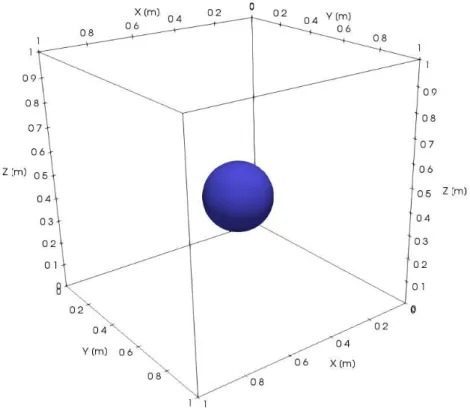
4.1 Diagram of the initial position of the sphere submitted to deformation. . . 53
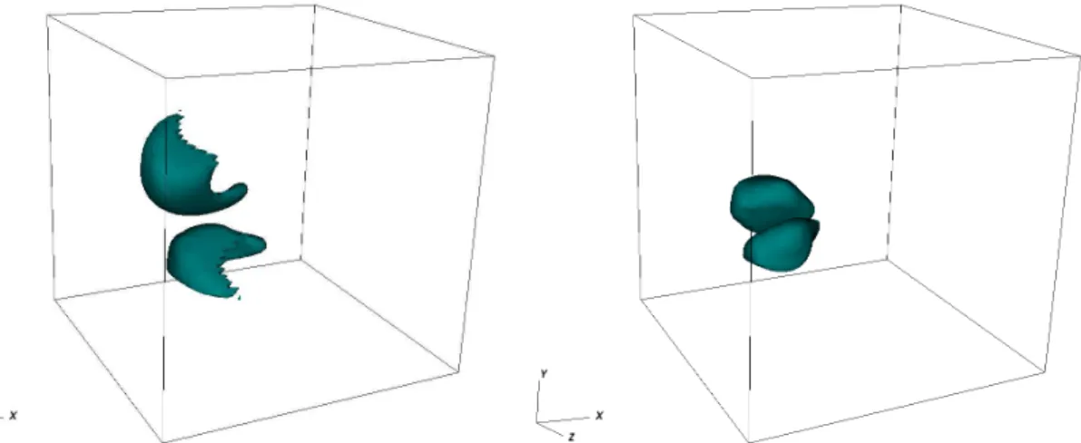
4.2 Temporal stages of the droplet deformation. . . 55
4.3 Diagram of the denser sphere surrounded by less dense phase in a cubic domain. 57 4.4 Magnitude of spurious velocities. . . 58
4.5 Map showing the bubble entrainment zone for different conditions based on
the Weber and Froude numbers, adapted from (OGUZ; PROSPERETTI, 1990). 60
4.6 Schematic of the droplet in the imminence of impacting the water pool. . . 61
4.7 The effect of the air pushing the free surface of the water pool. . . 62
4.8 Qualitative comparisons of the numerical splash topologies with images from Morton, Rudman and Liow (2000) for the case I. . . 62
4.9 Qualitative comparisons of the numerical splash topologies with images from Morton, Rudman and Liow (2000) for the case II. . . 63
4.10 Quantitative comparison of the numerical results for the depth crater with the experimental data of Morton, Rudman and Liow (2000). . . 63
4.11 Dimensions of the experimental domain for the two cases of LJIC. . . 65
4.12 Physical domain for the two cases of LJIC. . . 65
4.13 Map of momentum flux ratio versus Weber number for the primary breakup of the LJIC. . . 66
4.14 Grid and refinement zone near jet. . . 68
4.15 Comparison of volume fraction field atx−planeand mass fraction distribution and velocity at z−plane for both analyzed domains. . . 69
4.16 Pressure on liquid column jet and spray formation. . . 71
4.17 Profiles of liquid column jet. . . 72
4.18 Streamwise velocity component. . . 72
4.19 Streamlines of air flow around the liquid jet. . . 73
4.20 General view of the first and secondary breakups. . . 74
4.21 Sampling plane at 3.81cm, red line. . . 76
4.23 Schematic diagram of a drop with oblique velocity compared to the air streamline. 78
4.24 Average of droplet diameter in three planes forC2. . . 80
4.25 Mass fraction distribution forC1using different primary and secondary breakup models. . . 82
4.26 Mass fraction distribution for case C2 using different primary and secondary breakup models. . . 84
4.27 Droplet velocity forC1at the sampling plane3.81cmdownstream of the liquid jet nozzle. . . 85
4.28 Liquid jet curvature for C1. . . 87
4.29 Droplet velocity forC2at the sampling plane3.81cmdownstream of the liquid jet exit. . . 88
4.30 Mass fraction distribution using Cb = 3.44and AB-TAB model. . . 90
2.1 Important dimensionless parameters for LJIC study . . . 7
3.1 The analogy between the mass-spring-damper system and a oscillating and distorting droplet. . . 38
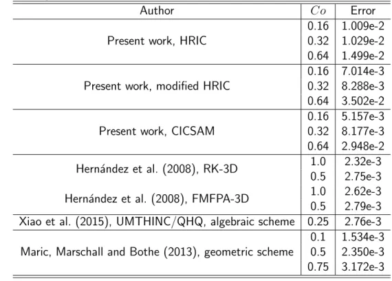
4.1 Error of numerical simulation compared to the analytical solution for different algebraic schemes and Courant numbers. . . 56
4.2 Comparison of the numerical solution and analytical solution for the problem of surface tension in a stationary inviscid droplet. . . 58
4.3 Scaled dimensions of the splash cases. . . 61
4.4 Physical properties of the fluids studied. . . 65
4.5 Flow conditions for the two studied cases. . . 66
4.6 Numerical settings for the two studied cases. . . 67
4.7 Mean diameter of droplet in the last plane (air tunnel exit) for C1. . . 79
4.8 Mean diameter of droplet in the last plane (air tunnel exit) for C2. . . 81
4.9 l2−normof the mass fraction distribution for C1. . . 83
4.10 l2−normof mass fraction distribution for C2. . . 83
4.11 l2−normof the mass fraction distribution for C2. . . 89
Abbreviations
AMR Adaptive Mesh Refinement
CAP Contribution of the ap coefficients
CICSAM compressive interface capturing scheme for arbitrary meshes
CIP Cubic Interpolated Pseudo-particle
CLSMOF Coupled Level Set Moment of Fluid
CLSVOF Coupled Level Set Volume of Fluid
CSF Continuum Surface Force
FVM Finite Volume Method
HRIC high resolution interface capturing
LES Large Eddy Simulation
LJIC Liquid jet in crossflow
LPP lean, premixed and pre-vaporized combustion
PDA phase Doppler anemometry
PDF probability density function
PDPA Phase Doppler Particle Analysis
PLIC Piecewise Linear Construction
RT Rayleigh-Taylor
SMD Sauter Mean Diameter
TAB Taylor Analogy Breakup
URANS Unsteady Reynolds Averaged Navier-Stokes
VOF Volume of Fluid
Greek letters
α volume fraction
δ to represent the Kronecker delta
ǫ dissipation rate of the turbulent kinetic energy
κ turbulent kinetic energy or interface curvature in the VOF model
Λ integral length of the turbulent jet [m]
λ wave length [m] or a specific coefficient for different models
µ dynamic viscosity [kg·m−1
·s−1]
ρ density [kg·m−3
]
σ surface tension coefficient [N ·m−1
]
τ relaxation time
τ stress tensor
ε surface breakup efficiency factor
Latin letters
Ca Capilarity number
Co Courant number
d diameter [m]
f source term
F a Faeth number
g gravity [m·s−2
]
J Liquid to air momentum ratio
L to indicate left side or length scale
m index for iteration or mass [kg]
M a Mach number
n to indicate normal vector
nf number of faces
Oh Ohnesorge number
p pressure [P a]
R right
r radius or distance (vector) [m]
Re Reynolds number
s distance [m]
t time [s]
u velocity component [m·s−1
]
v velocity component [m·s−1]
w velocity component [m·s−1
]
W e Weber number
x spatial coordinate component [m]
Y random number between 0and 1
y spatial coordinate component [m]
z spatial coordinate component [m]
Subscripts
∞ to indicate a bulk or mean value of the air crossflow
b to indicate primary breakup
c to indicate the jet column
crit to indicate a critical value
d to indicate drag
f to indicate face value
g to indicate the gas phase
i index notation
j index notation
jet to indicate a variable of the jet flow
L to indicate length scale
l to indicate the liquid phase
R to indicate right side
rel to indicate relative values
s to indicate the surface of the jet column
sc surface control
st surface tension
st to indicate surface tension
t to indicate turbulent variable
vc volume control
w, b to indicate the combined buoyancy-weight force
Superscripts
′
to indicate fluctuating value
′′
to indicate flux over a surface area
¯ to indicate the mean value
n current time for the variables
LIST OF FIGURES viii
LIST OF TABLES x
1 INTRODUCTION 1
1.1 Objectives . . . 3
1.2 Dissertation structure . . . 3
2 LITERATURE REVIEW 5 2.1 LJIC fundamentals . . . 5
2.2 Experimental analysis of LJIC . . . 7
2.3 Numerical analysis of LJIC . . . 15
2.3.1 Euler-Lagrange approach . . . 16
2.3.2 Euler-Euler approach . . . 18
2.3.3 Hybrid approach . . . 21
2.3.3.1 Low dependence on transition models . . . 21
2.3.3.2 High dependence on transition models . . . 22
3 MODELING AND METHODOLOGY 25
3.1 Physical modeling . . . 25
3.2 Mathematical modeling . . . 27
3.2.1 Eulerian referential . . . 28
3.2.1.1 Turbulence closure model . . . 29
3.2.1.2 Two-phase model . . . 32
3.2.2 Lagrangian referential . . . 34
3.2.3 Primary breakup and secondary breakup models . . . 36
3.3 Numerical modeling . . . 41
3.3.1 Eulerian referential . . . 41
3.3.1.1 Temporal term . . . 41
3.3.1.2 Advection term . . . 42
3.3.1.3 Diffusion term . . . 43
3.3.1.4 Advection scheme for VOF method . . . 43
3.3.1.5 Pressure-velocity coupling . . . 45
3.3.1.6 Momentum interpolation method . . . 46
3.3.2 Lagrangian referential . . . 48
3.3.2.1 Integration scheme . . . 48
3.3.2.2 Interpolation at the particle position . . . 48
3.3.2.3 Algorithm of particle tracking . . . 49
3.3.3 Numerical overview . . . 50
3.3.4 Methodology . . . 50
4.1 Verification and validation of VOF method . . . 52
4.1.1 Sphere deformation . . . 53
4.1.2 Surface tension in a stationary droplet . . . 57
4.1.3 Water droplet splash . . . 59
4.2 Numerical results for LJIC . . . 64
4.2.1 LJIC cases and numerical settings . . . 64
4.2.2 Strategy for domain reduction . . . 67
4.2.3 LJIC characteristics using hybrid approach . . . 70
4.2.4 Evaluation of primary breakup coefficients and secondary breakup models 75 4.2.4.1 General results for mean diameter distribution . . . 76
4.2.4.2 Mass fraction distribution . . . 81
4.2.4.3 Droplet velocity . . . 85
4.2.5 Two-way coupling and droplet collision effects . . . 89
INTRODUCTION
Humanity has constantly sought improvements in living conditions, even in war. In the
beginning of the World War II, the German aircraft Messerschmitt Bf 109, Fig. 1.1 had a big
advantage over British fighters, concerning the type of fuel injection. The German aircraft had
a different fuel injection, so that fuel injection into the engine did not fail, even in extreme
manoeuvres, such as fly upside-down or to perform other negative-G manoeuvres.
The majority of processes and equipment in nature and industry is related with
fluids and their interactions, which affect directly the efficiency of these processes and
equipment. Regarding fluids in the possible existing systems, usually two-phase flow condition
is encountered. Two-phase flow presents additional physical aspects to those in one-phase flow,
such as interfacial interaction and high physical properties ratios. The interfacial interaction
is extremely hard to study, since the interface is very thin, whose interactions occurs in
microscopic level. However, the interface and their interactions are not treated in microscopic
level, so that some physical concepts are inferred to keep analysis on continuum hypothesis,
as an example by the use of the surface tension coefficient.
Spray is an important two-phase flow system that are present in many practical problems,
such as: combustion, irrigation and airway medication. The efficiency of each process depend
on several spray characteristics, for example: injection type, spray angle, droplet diameter,
droplet velocity, and time/space to produce entirely the desired droplet distribution. Liquid jet
in crossflow (LJIC) is used to obtain liquid spray in short length scale using simpler injection
system, with lower pressure injection, than that used in diesel injection. Due to these features,
LJIC has been used in gas turbine combustors, scramjet and ramjet combustors (HOJNACKI,
1972). The combustion efficiency of these combustors are highly dependent on the droplet
formation. Therefore, the understanding of the breakup process is crucial to develop models
able to predict the spray formation. Numerical simulations, with reliable models related to
LJIC, can provide many useful information to enhance the combustors efficiency.
For better understanding of spray formation in LJIC, experimental analyses are extremely
important. However, experimental analyses are often expensive and present geometric
restrictions. When reliable models and correlations are well established, numerical simulations
are an interesting approach for projects and provide relevant results that are difficult or
impossible to obtain experimentally. Therefore, the development of numerical modeling able
to predict suitably spray formation in LJIC is valuable for industrial and research purposes.
In this dissertation, the evaluation of some methodologies to solve numerically spray
1.1 Objectives
The purpose of this dissertation is to fill the gap related to numerical modeling in spray
formation in LJIC. Currently, three numerical approaches have been used to solve LJIC:
Euler-Euler, Euler-Lagrange and hybrid approach. The author of this dissertation aims to fill some
gaps on the hybrid approach use, such as: evaluation of primary breakup coefficients, analysis
of a new secondary breakup model proposed by Dahms and Oefelein (2016) and the evaluation
of four way coupling on LJIC, using a hybrid approach.
Therefore, the main objective of this dissertation can be stated as: investigate
numerically, by means of a hybrid approach, spray formation in LJIC configuration with respect
to primary breakup modeling, secondary breakup model and the effect of two-way coupling
along with droplet-to-droplet collision.
Furthermore, the following specific goals can be listed:
• implement subroutines for the VOF method Euler-Lagrange conversions and secondary
breakup models on an unstructured grid code;
• verify and validate VOF implementation;
• make an appropriate computational grid to solve LJIC by means of hybrid approach;
• find detailed LJIC experimental cases for validation;
• and establish the spray features to compare the chosen models.
1.2 Dissertation structure
This dissertation was developed following a coherent structure composed by five
chapters. In the present chapter, an introduction of the dissertation is made, covering the
In chapter 2, a relevant bibliographic review about sprays in LJIC is presented. Firstly,
physical fundamentals for LJIC are described, highlighting the main dimensionless variables
related to LJIC problems. Secondly, the main results and correlations of experimental
researches for spray in LJIC are shown from the former publications to the most recent ones,
emphasizing how research has remained firmly. Finally, the numerical researches about the
theme are discussed, where advantages and disadvantages of the three approaches, i.e.,
Euler-Euler, Euler-Lagrange and hybrid are shown.
In chapter 3 physical, mathematical and numerical modelings used in all simulations
performed in this work are presented.
In the Chapter 4, all results are presented and discussed in detail. Verification of the
VOF model implementation are presented, guaranteeing that VOF model implementation is
correct and reliable. In the following, all numerical simulations for spray formation in LJIC are
described, according to the evaluated correlations/models.
The main conclusions of the work along with some suggestions for future works related
LITERATURE REVIEW
This chapter is dedicated to contextualize the contribution of this dissertation in the
most recent numerical research of liquid jet in crossflow (LJIC). Thus, the LJIC fundamentals,
some experimental works and the numerical methods available to solve LJIC, with their
respective numerical results of the state of the art, are presented in the following.
2.1 LJIC fundamentals
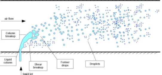
Liquid jet in crossflow (LJIC) consists of a liquid jet that interacts with a gas flow
obliquely, as represented in Fig. 2.1. In this physical configuration, the interaction of phases
and the properties differences between liquid and gas establish high gradients of physical
properties in the interface that is infinitesimally thin, presenting a discontinuous properties
jump. Instabilities may arise in LJIC, taking to the breakup of the intact liquid column and
stripping droplets from the liquid surface concurrently, depending on the flow features. In
LJIC, some physical phenomena can exist simultaneously: at the liquid-air interface, surface
tension collaborates with the maintenance of the structure of the liquid jet column and liquid
drops; turbulence eddies and aerodynamic instabilities favors the disruption of the liquid jet;
Figura 2.1 – Diagram of the analyzed LJIC domain.
each phase sharing interface.
In addition to the interface phenomena, primary breakup is inherently part of LJIC,
consisting of the first ruptures of the intact liquid column, which creates the first droplets. This
breakup process is very misunderstood due to the difficulties of visualizing droplets formation
properly and obtaining not intrusive experimental flow data. However, it is known that primary
breakup may occur due to the growth of Kelvin-Helmholtz, Rayleigh-Taylor, turbulent eddies
instabilities and cavitation (BRAVO; KWEON, 2014).
Some of those droplets suffer secondary breakup, depending on the instabilities growth,
related to the surface tension, aerodynamic and viscous forces balance. The droplets interact
with the surrounding air flow and with one another, experiencing coalescence, elastic collision,
or a composition of the last two modes.
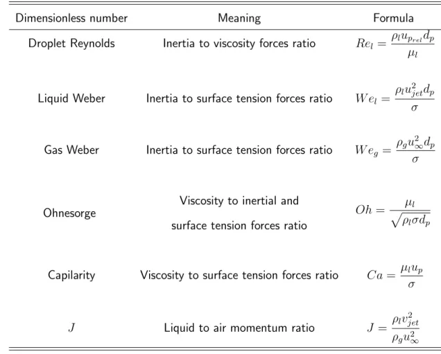
Considering the complexity of the problem, some dimensionless numbers related to the
physical phenomenon are very useful. Some important dimensionless numbers for LJIC are
presented in Tab. 2.1, where,ρl, µl and d are respectively the density, dynamic viscosity and
diameter of the liquid drop; ρg is the gas density and σ is the surface tension coefficient of
Tabela 2.1 – Important dimensionless parameters for LJIC study
Dimensionless number Meaning Formula
Droplet Reynolds Inertia to viscosity forces ratio Rel=
ρlupreldp
µl
Liquid Weber Inertia to surface tension forces ratio W el =
ρlu2jetdp σ
Gas Weber Inertia to surface tension forces ratio W eg =
ρgu2∞dp
σ
Ohnesorge Viscosity to inertial and Oh= pµl
ρlσdp
surface tension forces ratio
Capilarity Viscosity to surface tension forces ratio Ca= µlup
σ
J Liquid to air momentum ratio J = ρlv
2 jet ρgu2∞
Method and equipment improvements have gradually overcome the experimental and
numerical challenge of LJIC spray formation analysis. In the next sections, some numerical
and experimental outcomes in LJIC field are presented, over the years.
2.2 Experimental analysis of LJIC
First experimental works on LJIC were unable to analyze deeply spray formation, being
limited to correlate the liquid jet penetration in the air crossflow.
Chelko (1950) obtained a jet penetration correlation, using photographs taken from
LJIC through transparent tunnel walls. Jet penetration was correlated using the velocities and
jet nozzle center line,x, and the jet diameter, djet, according to Eq. 2.1,
y djet
= 0.450
vjet v∞ 0.95 ρl ρg 0.74 x djet 0.22 , (2.1)
where: y is the distance of the liquid jet from the exit; djet is the jet diameter; vjet is the jet
velocity; v∞ is the velocity of the gas crossflow; ρl is the liquid density; ρg is the gas density
and x is the longitudinal distance of the liquid jet. This correlation presented a deviation of
approximately7% from the experimental measurements.
The lateral penetration of a water jet in a supersonic air crossflow (i.e. the spray width
from a top view of the jet diameter) for different Mach numbers was correlated by Rebello
(1972). The author proposed equations for the jet penetration as function of the Mach number,
injection pressure, jet diameter and angle of injection, identifying that the injector diameter
and the angle of injection are the dominant parameters on the lateral jet penetration. The
general empirical correlation for lateral penetration presented a degree of agreement of 0.86
compared with experimental data.
The experimental limitations of obtaining a better understanding of the spray formation
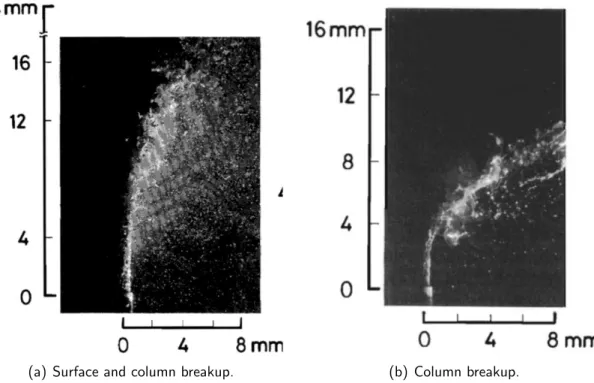
in LJIC were reduced with the improvement of equipment and methodologies. Oda et al.
(1994) studied the breakup of a liquid jet normal to a high-speed airstream using a laser-sheet
tomography and Fraunhofer techniques (i.e. related to diffraction measurements). The authors
used Eosine-Y(C20H6Br4N a2O), a fluorescent dye, dispersed in water for better visualization
of the breakup process. Two breakup mechanisms were identified for different flow conditions,
according Fig. 2.2. In the first identified mechanism, surface and column breakup, the liquid
jet was ejected into a high speed airstream, distorting of the liquid column towards a bow
shape. Small droplets also detached from the tips of the bow, large drops were produced from
the end of the liquid column and bellow the end of the liquid column a cavity in the liquid
column was identified. In the second mechanism, column breakup, lower velocities of the liquid
jet and the airstream were imposed, resulting in an unstable liquid column (snakelike shape).
(a) Surface and column breakup. (b) Column breakup.
Figura 2.2 – Visualizations of breakup mechanisms identified by Oda et al. (1994).
verified the intact liquid column height (before full breakup) is inversely proportional to the
airstream velocity and directly proportional to the injection velocity.
In the work of Wu, Kirkendall and Fuller (1997), breakup process of LJIC in a subsonic
air crossflow were experimentally studied, varying test liquids, injector diameter and Mach air
number to obtain a wide range of operation conditions. Pulsed shadowgraphic technique was
used to visualize and analyze the breakup properties and formation. In Fig. 2.3, different
conditions of Weber and momentum ratios numbers are shown from the results of Wu,
Kirkendall and Fuller (1997). The authors identified two primary breakup mechanisms, different
from those of the work of Oda et al. (1994), termed shear breakup and column breakup,
classifying them using Weber and liquid to air momentum ratio numbers. Just the column
breakup was correlated using an analogy with the individual droplet breakup, when subjected
to aerodynamic forces. Column breakup equations are expressed in function of the vertical
(along to the jet), y, and horizontal (perpendicular to the jet), x, breakup position of the
(a)J = 9.9andW e= 71. (b) J = 70.8andW e= 160.
Figura 2.3 – Visualizations of breakup mechanisms identified by Wu, Kirkendall and Fuller (1997).
Eq. 2.4, was correlated,
yb djet
= 3.44√J, (2.2)
xb djet
= 8.06, (2.3)
y djet
= 1.37
s
J
x djet
, (2.4)
where, the origin of the axes is the center of the exit jet diameter.
An experimental investigation of non-turbulent LJIC at normal temperature and pressure
was carried out by Mazallon et al. (1998), using pulsed shadowgraphs to observe jet
deformation and breakup. In their work, an wide range of dimensionless variables was evaluated,
changing several parameters (different liquids, jet diameters, inlet jet velocities, air velocities):
momentum ratio,J = 100−8000; and liquid to gas density ratios, ρl/ρg = 580−1020. The
authors inferred primary breakup process in LJIC was similar to the droplet breakup process
(secondary breakup). Four breakup regimes were identified and characterized only through the
Weber number (Ohnesorge, density ratio and liquid to gas momentum ratio presented little
influence in the breakup regime): column breakup, W e > 5; bag breakup, 5 < W e < 60; bag/shear breakup,60< W e <110; and shear breakup,W e >100. Furthermore, the authors correlated two kinds of waves in the LJIC, observed in the experiments: column wave length,
λc, and surface wave length, λs, Eq. 2.5 and Eq. 2.6, respectively,
λc/djet = 16.3W e−0.79, (2.5)
λs/djet = 2.82W e−0.45. (2.6)
These waves are related to the onset of the primary breakup in the LJIC, though none
correlation of the drop diameter from the primary breakup was made in the work of Mazallon
et al. (1998).
Becker and Hassa (2002) investigated experimentally breakup, penetration and
atomization of a plain jet of kerosene jet A-1 fuel in an air crossflow at test conditions relevant
to lean, premixed, pre-vaporized (LPP) combustion of gas turbines, using time-resolved
shadowgraphs, Mie-scattering laser lightsheets and phase Doppler anemometry (PDA). Test
were conducted in a quartz duct with rectangular cross section of 25 by 40 mm, where 27 were
performed. Velocity, pressure and temperature of the air were respectively u∞ = 50,75,100
m/s,pg = 1.5to15barandTg = 290K. The authors confirmed, similarly to Wu, Kirkendall
and Fuller (1997) and Mazallon et al. (1998), two breakup mechanisms, column breakup and
surface breakup, obtaining through Eq. 2.7,
W ecrit = 10
3.1−log(J) 0.81
, (2.7)
a good agreement of their data with the mechanisms classification made by Wu, Kirkendall
longitudinal distance from the diameter jet, x/djet = 2−22, liquid to air momentum ratio, J = 1−40 and We number,W e= 90−2120, as expressed by Eq. 2.8,
y djet
= 1.48J0.42ln
1 + 3.56 x
djet
, (2.8)
presenting a standard deviation of1.21from the experimental data points.
An experimental investigation of the primary breakup of non-turbulent round liquids
jets in gas crossflow was conducted by Sallam, Aalburg and Faeth (2003) considering different
liquids, jet diameters, liquid jet velocities and air crossflow velocities, that yields the following
range of dimensionless parameters: liquid to gas density ratio, ρl/ρg = 683−1021; Weber
number,W e= 30−260; liquid to air momentum ratio, J = 3−200; and Ohnesorge number,
Oh = 0.003−0.12. Pulsed holography and shadowgraphy techniques were used to observe primary breakup of the LJIC, obtaining experimental uncertainties less than 10%for diameter larger than0.01mmand for drop velocity, with95%confidence. Similarities between primary breakup of the LJIC and breakup of individual drops subjected to shock wave disturbances
were found, as Mazallon et al. (1998). Visualizations showed there is no influence of liquid
jet turbulence or vorticity in the primary breakup of the liquid jet, even for jet Reynolds
number of 30000. The authors identified three breakup regimes: bag, multimode and shear breakup, strongly related to the Weber number and not (or weakly) related to the liquid to
air momentum ratio and Ohnesorge number, for conditions tested. Despite three breakup
regimes were identified, the authors correlated two primary breakup mechanisms: breakup of
the entire liquid column and shear breakup in the liquid jet surface. The distance from the
exit jet diameter to the column breakup was correlated, similarly to Wu, Kirkendall and Fuller
(1997), using the liquid to air momentum ratio, according Eq. 2.9,
yb djet
= 2.6√J. (2.9)
For the shear breakup correlation, the diameter of the ligaments formed along the column
diameters were comparable to the drop sizes caused by the primary breakup along the liquid
surface, assuming Rayleigh breakup caused drops to be formed from the end of the ligaments.
Thus, the drop sizes from the primary breakup along the liquid jet are expressed by Eq. 2.10
and Eq. 2.11,
dp djet
= 3.36
νly vjetd2jet
1/2
, y/yc ≤1, (2.10)
dp djet
= 0.132, y/yc >1, (2.11)
where,νl is the kinematic viscosity of the liquid,vjet is the jet velocity at the diameter jet exit
and yc/djet = (0.001vjetdjet)/(νl). Beside this, drop velocities after breakup were measured.
The resulting correlations for drop velocities in jet direction and in air crossflow direction are
expressed, respectively by Eq. 2.12 and Eq. 2.13
vp vjet
= 0.7, (2.12)
up uL
= up
u∞(ρg/ρl)1/2
= 6.4. (2.13)
Deformation and breakup properties of turbulent LJIC were studied experimentally by
Aalburg, Faeth and Sallam (2005), using pulsed shadowgraph and holograph observations, for
the following conditions: gas Weber number, W e = 0−282; liquid to gas density ratios of
683 and 845; jet exit Reynolds number, Re = 3800−59000; and small effects of the liquid viscosity, Oh <0.12. Aalburg, Faeth and Sallam (2005) found a negligible effect of the gas crossflow on changing the liquid jet velocity in the jet flow direction, which means the liquid jet
velocity, vjet, is approximately constant. They proposed a correlation for drop SMD (Sauter
Mean Diameter) in function of the distance along the liquid jet, Eq. 2.14,
SM D
Λ = 0.52
y
ΛW e
1/2 Λ
0.52
, (2.14)
liquid jet, Λ. Droplet diameter was not affected by the crossflow, suggesting that turbulent primary breakup dominates aerodynamic effects in the conditions evaluated. Beside this, the
authors showed that drop velocities after turbulent primary breakup were independent of the
droplet size, with drop velocity in the liquid jet direction comparable to the liquid jet velocity
at the exit, Eq. 2.15, while the droplet velocity in the air flow direction were correlated through
Eq. 2.16,
vp vjet
= 0.6, (2.15)
up uL
= up
u∞(ρg/ρl)1/2
= 4.27. (2.16)
An experimental investigation of the primary breakup of turbulent and non-turbulent
LJIC, at normal pressure and temperature, is described by Sallam et al. (2006), for Weber
numbers of0−2000, liquid to gas momentum ratios of100−8000, liquid to gas density ratios of 683−1021, Ohnesorge numbers of0.003−0.12, jet Reynolds numbers of 300−300000. Jet primary breakup regimes, conditions for the onset of breakup and properties of waves were
obtained using pulsed shadowgraph and holograph observations. The authors recognized three
breakup regimes, namely bag breakup, multimode breakup and shear breakup, both functions
of the Weber number, with little influence of the viscosity (at small Ohnesorge numbers,
Oh <<1) on the transition of the breakup regime. For large Ohnesorge numbers,Oh >>1, the breakup regime of non-turbulent LJIC is function of W e1/2/Oh. For non-turbulent LJIC,
the authors noted drop velocity distributions after breakup were relatively independent of drop
size, according Eq. 2.17 and Eq. 2.18, respectively for crossflow velocity and jet flow velocity
directions,
up uL
= up
u∞(ρg/ρl)1/2
= 6.4, (2.17)
vp vjet
= 0.6. (2.18)
breakup), along the liquid column, increases with increasing distance from the jet diameter
exit in transient state. Two breakup regimes of turbulent LJIC were found, aerodynamic
breakup regime and turbulent breakup regime. A new dimensionless parameter, Faeth number,
F a=W eΛJ1/3, was proposed to divide these two regimes: forF a >17000, turbulent breakup
regime occurs and forF a < 17000 aerodynamic breakup regime occurs. Breakup conditions for turbulent LJIC were correlated similarly to Sallam, Aalburg and Faeth (2003), Aalburg,
Faeth and Sallam (2005), only different coefficients were obtained for the correlations of the
droplet SMD, Eq. 2.19, and of the drop velocities, Eq. 2.20 and Eq. 2.21,
SM D
Λ = 0.56
y
ΛW e
1/2 Λ
0.5
, (2.19)
up uL
= up
u∞(ρg/ρl)1/2
= 4.82, (2.20)
vp vjet
= 0.75. (2.21)
Experimental researches about LJIC have been made progressively (RAGUCCI;
BELLOFIORE; CAVALIERE, 2007; NG; SANKARAKRISHNAN; SALLAM, 2008; PRAKASH
et al., 2015; SINHA et al., 2015; BEHZAD; ASHGRIZ; MASHAYEK, 2015; ENAYATOLLAHI;
NATES; ANDERSON, 2017), however the main experimental works of LJIC related to this
dissertation were presented above, since breakup position of LJIC and diameter size in the
primary breakup are the most important LJIC characteristics for this dissertation.
2.3 Numerical analysis of LJIC
Due to the complexity of LJIC, there are three approaches to solve numerically this
spray configuration, depending on the desired results: Euler-Lagrange approach, Euler-Euler
2.3.1 Euler-Lagrange approach
In Euler-Lagrange approach, one phase is treated as continuous that is evaluated in a
fixed referential system (Eulerian referential), and the other phase is treated as discrete using
a mobile referential system (Lagrangian referential) where discrete particles are tracked within
the computational domain. Momentum, mass and energy exchanges between phases may be
modeled whenever they are relevant for the specific problem. This approach is more suitable
for immiscible phases flows with low concentrations of a phase over the other. Usually, particle
(gaseous, liquid or solid) flows are treated in this approach. The computational cost is low
for relative low numbers of immersed particles in the continuous phase; however it can be
prohibitive for high amounts of discrete particles.
In LJIC, Euler-Lagrange approach treats the gas phase as continuous and liquid phase
as discrete. In the jet exit, liquid column jet and its interaction with the air crossflow is not
well represented by discrete liquid particles, since the flux of discrete particles do not represent
a cohesive body as liquid column jet. However, far from the jet exit, liquid spray is better
represented by discrete liquid particles, because in fact, in this region there is a predominance
of liquid particles (drops). In the past, this approach was widely used to represent spray,
mainly due to the computational cost limitations. Currently, the Euler-Lagrange approach is
commonly used to obtain practical or preliminary results.
A numerical analysis of the LJIC was made using Euler-Lagrange approach by Reitz
(1987). They injected liquid phase into the air crossflow using the blob method, which consists
injecting discrete liquid drops with a diameter of the injector exit diameter order, with a
frequency injection that conserves mass upstream of the injector exit. Drop collision and
coalescence were accounted in the numerical computations. Breakup of the original droplets
followed linear stability analysis, which was able to describe different breakup regimes. Different
diameter for the generated droplets after breakup were calculated, relating the wavelength of
unstable waves on the blob surface with the generated droplet diameters. Jet penetration
concluded drop size, also well correlated with experimental data, is found to be determined by
a competition between drop breakup, drop coalescence and vaporization effects.
Euler-Lagrange approach was used with the Large Eddy Simulation (APTE;
GOROKHOVSKI; MOIN, 2003), that is a turbulence closure model in which large scales
are calculated and only small scales are modeled. Secondary breakup of the injected drop in
crossflow was evaluated through a stochastic model in the form of the differential
Fokker-Planck equation for the probability density function (PDF) of droplet radii. Parameters of the
model were obtained according to the local Weber number, using two-way coupling between
gas and liquid phases. The authors used LES simulation to provide accurate predictions of
turbulent transport used in the estimation of the maximum stable diameter of droplets before
breakup. Numerical results of jet penetration and spray angle agreed well with experimental
work of Hiroyasu and Kadota (1974).
Balasubramanyam and Chen (2008) analyzed numerically a LJIC using Euler-Lagrange
approach and κ −ǫ turbulence closure model. The entrance of the liquid particles from
the injector exit inside the air crossflow followed the blob method. The grid size used to
solve this problem was of 208000 elements, that is a relatively coarse grid for computational fluid dynamics. The authors obtained good comparisons with experimental results referent
to droplet velocity along the air duct height. However, the jet penetration was not very well
represented by the numerical results.
Jaegle et al. (2010) analyzed numerically LJIC using Euler-Lagrange approach with LES
turbulence closure model. The authors modeled the jet column effect over the air crossflow
through an imposition of a liquid jet curved column (virtually). Droplets were released from a
breakup point at the top and along of the jet column, since the Euler-Lagrange is not able to
predict dense region properly. A fully developed particle size distribution was assumed, where
size droplets were selected in the injection instant. Liquid volume flux and the SMD were
compared to experimental data (BECKER; HASSA, 2002) presenting reasonably agreement.
drop stripping process and secondary breakup was simulated using Taylor Analogy Breakup
(TAB) and Rayleigh-Taylor (RT) models concomitantly. Compressible flow and LES turbulence
closure model were implemented in the code used, which included modified drag coefficient
and breakup models depending on compressible effects and droplet deformation. The authors
obtained good comparisons with experimental data referent to the jet penetration height and
SMD along to the air flow direction.
2.3.2 Euler-Euler approach
Euler-Euler approach consists evaluating both phases, considered as continuous phases,
under a fixed referential system. This approach is more suitable for immiscible flows and
in the regions where phases have similar concentrations. The concept of volume fraction of
the phases is assumed, so that different phases can not occupy the same place at the same
time, unless in the interface. Advective transport equations for the phases (phase, if two-phase
flow) are solved, ensuring the laws of classical mechanics be respected. This approach presents
positive aspects in representing LJIC, such as: liquid breakup is calculated (without empirical
modeling); interface is better represented along all domain; and droplet interaction with walls
and other droplets (coalescence, bouncing) do not need additional modelings. However, these
positive aspects are achieved only at high computational costs. Several methods have been
developed in the sense of Euler-Euler approach, where each of them presents an extensive
description, therefore just a summary of the results of some methods are discussed in the
following.
Pure application of the Euler-Euler approach to LJIC (and other liquid jets
configurations) has been possible recently due to the computer improvements and parallel
computation strategies (many processors to solve a problem). The numerical solution of
two-phase flows properly using Euler-Euler approach requires high number of elements. Shinjo and
Umemura (2011) evaluated numerically diesel jet tip atomization, using VOF method, with a
turbulence and cavitation instabilities. Advection terms were solved using Cubic Interpolated
Pseudo-particle (CIP) method. Two-phase flow was solved through Multi-interface Advection
and Reconstruction Solver combined with a Level-Set method, while the surface tension was
evaluated in all domain with the Continuum Surface Force (CSF) method. The minimum grid
resolution required in the simulations performed by the authors was 400 million of elements in the JAXA supercomputer system. The temporal evolution of the jet breakup, the umbrella
formation at the jet tip and the droplet formation along the jet due to the air interaction
(airflow recirculation) were well capture in the simulations.
The Volume of Fluid method was used by Hirt and Nichols (1981) to study the
formation and fragmentation of the spray from two impinging jets (CHEN et al., 2013).
Adaptive Mesh Refinement (AMR) technique were used with VOF method for capture all
physical characteristics of the impinging jets with high fidelity. The advection equation for
the volume fraction, from the VOF method, was discretized using a robust Piecewise Linear
Construction (PLIC) scheme, resulting in a good representation of the interface (POPINET,
2009). The surface tension term in momentum equation was discretized with a combination
of a balanced force surface tension discretization and a height function curvature estimation,
which presented a second order convergence rate, reducing considerably parasitic currents,
that appears in the simulation of a stationary droplet in theoretical equilibrium (POPINET,
2009). These highly accurate schemes (with other high order spatial and temporal schemes)
in combination with AMR, based on Octree meshes (one of the type meshes for AMR with the
lowest computational cost), were able to capture all the flow patterns formed by impingement
of two liquid jets, presenting good correlation with experimental data, such as: fine structures
on their characteristics length scales; and various atomization modes, including sheet formation
and rupture, atomization into ligaments and droplets. Although in his work AMR was used,
it was necessary more than 1million of cells to accurately solve spray formation of impinging jets (more than134 million would be required in a uniform grid). LJIC presents smaller length scales than impinging jets, thus a higher number of cells would be necessary, even with the
High fidelity simulations of Diesel jet were made by Arienti and Sussman (2015) using
two interface tracking: ELVIRA method (EDWARD; JR; PUCKETT, 2004), for liquid-gas
interface; and Coupled Level Set Moment of Fluid-CLSMOF (JEMISON et al., 2013), for
interfaces with solid phases. Besides this, embedded boundary method was used to simulate
walls, since boundary movement was involved. Diesel jet required a domain with a mesh size
of 576×64×64 (more than 2.3 million elements), which were solved using 128 SUN X6275 blades (total of 256 cores) in parallel. Droplet formation along to the jet were well described,
though the calculated rate of injection and momentum were smaller than predict values from
models based on the injection pressure and an assigned discharge rate. The differences in the
rate of injection and momentum with the models may be related to the low mesh size used for
the authors, in comparison to the mesh size used in the work of Shinjo and Umemura (2011).
Similar simulations of a fuel jet using an unstructured un-split VOF method was made
(BRAVO et al., 2015) for realistic complex injector. The conditions analyzed consisted of a
jet diameter of90µm, that released fuel in a quiescent chamber filled of Nitrogen at ambient conditions (20bar,300K) with6.9×104 < Re <2.5×10⁵ and5.4×104 < W e <1.25×10⁵. For the turbulence closure model, the Smagorinsky LES model was used, which together with
a good interface representation in VOF method required a 77million grid points. Qualitative comparisons showed numerical breakup length was twice as long as that of the experimental
images for lower injection pressure analyzed. These differences may arise due to the lack
of some physical modeling, such as turbulence flow upstream exit injector, cavitation and
fluid-structure interaction.
Due to the high number of elements required to solve LJIC (more than that used in
liquid jet in a quiescent air chamber), Euler-Euler approach has been hardly employed. Li
and Soteriou (2016) simulated LJIC using Euler-Euler approach and hybrid approach to be
described in the following section. Euler-Euler approach employed consisted in Coupled Level
Set Volume of Fluid (CLSVOF) method to capture spatial and temporal evolution of the
liquid-air interface and sharp interface ghost fluid method to stably handle with the high
the finite volume of 39µm, which corresponds to 503.3 million of elements, and an adaptive mesh refinement strategy (AMR), using three levels of refinement, resulting in 7.1 million of elements. For the uniform grid simulations 5000 cores were used and for AMR simulations,
24cores, both on a supercomputer. Numerical results were well compared with experimental data qualitatively and quantitatively. The authors recognized that for uniform grid simulations,
503.3million grid not only present high computational cost, but pose significant challenges in storing and processing the large set of simulation data. Therefore, for these simulations only
two dimensional data (surfaces) were extracted from the results and analyzed.
2.3.3 Hybrid approach
Hybrid approach has been used recently to solve jet breakup as a better way to capture
liquid-air interaction properly at more acceptable computational costs. Hybrid approach can
be divided in two class: low dependence on transition models (higher computational cost);
and high dependence on transition models (lower computational cost).
2.3.3.1 Low dependence on transition models
In this class of hybrid approach, the transition of a liquid portion from an Eulerian
analysis to a Lagrangian analysis follows the concept of Herrmann (2010), that developed a
parallel Eulerian-Lagrangian multi-scale coupling procedure for two-phase flows. The authors
used Eulerian approach to solve liquid-air interactions until some criteria (size of liquid drops)
and restrictions (grid capacity to solve interface interaction) be achieved, when Eulerian liquid
portions are converted into Lagrangian liquid droplets. The transition method described by
Herrmann (2010) consists in identifying an isolated liquid portion, which is converted into
Lagrangian particle according to two criteria: size criterion, that select a liquid portion if its
volume is lower than a threshold volume; and shape criterion, that select a liquid portion if
its eccentricity is lower than a threshold eccentricity. Both criteria indicate that the liquid
Refined Level Set Grid (RLSG) method for transporting liquid-air interface in a parallel code
(HERRMANN, 2008). Beside this, back transition (Lagrangian particle to Eulerian droplet)
were considered in the simulations, based on the size of a coalesced drop. The applicability
of the method was demonstrated with a detailed simulation of the atomization of a turbulent
liquid jet, similar those obtained in pure Euler-Euler approach.
Following the concept of Herrmann (2010), small liquids structures formed by
atomization were removed from Eulerian description and transformed into Lagrangian particles
using CLSVOF method with block structured AMR (LI; ARIENTI; SOTERIOU, 2010). Three
criteria were used to determine the eligibility of a liquid portion to be converted from Eulerian
approach to Lagrangian approach: volume size, sphericity and maximum local concentration
of droplet which the transformation to the Lagrangian phase can occur. Impinging jets and
LJIC were analyzed using hybrid approach. For Impinging jets, the computational time was
approximately150 seconds per time step, considering time step was 0.66µs and two levels of refinement were used, leading to a minimum grid size of31.25µm (in a uniform grid, it leads more than150million of grid points). For LJIC, computational time was300−400seconds per time step, considering time step was0.17µs and a base grid more than 4million of elements were used with three levels of refinement. Both simulations were performed on two8-core,32
Gb,3000 MHz nodes with InfiniBand switch. Qualitatively, both simulations presented good comparisons with experimental data. Sauter Mean Diameter measurements in a plane and
droplet distribution presented good correlation with experimental data, respectively for LJIC
and Impinging jets. Compared to Euler-Euler approach, hybrid approach effectively reduces
computational costs, even they are still high when low dependence on transition models are
used.
2.3.3.2 High dependence on transition models
Euler-Lagrange approach with high dependence on transition models does not represent
all the physics involved. However, this approach is able to determine many features of the
costs related to the high dependence on transition models in Euler-Lagrange approach is low,
comparable with the numerical simulations from Lagrange approach. The advantages of the
two separated approaches (Euler and Lagrange) is maintained, but some empirical models
are needed. The precursor work related to this methodology applied to LJIC is attributed to
Arienti et al. (2006). They implemented in the hybrid approach empirical correlations from
Sallam, Aalburg and Faeth (2003) and Sallam et al. (2006), described in section 2.2. The
methodology consisted in evaluated the empirical correlations for primary breakup at the top
of the liquid jet and along the column of the liquid jet. The stripped mass from the liquid
column was calculated using the surface breakup efficiency factor, Eq. 2.22,
ε= m˙
′′
l ρlu¯p
, (2.22)
where, u¯p is the mean stream-wise droplet velocity, Eq. 2.23,
¯
up =Cuu∞(ρg/ρl)
1/2
, (2.23)
and Cu is an empirical constant, reported by Sallam, Aalburg and Faeth (2003) as Cu = 6.4
for ρl/ρg > 500. The primary breakup at the top of the liquid jet was calculated according
described in the section 2.2, using the Eq. 2.9 (the authors assumed the empirical constant
as 2.44 instead 2.6) and Eq. 2.24, respectively for the breakup height and the drop diameter,
dp djet
= (1.5λb)1/3, (2.24)
where,λb =λc/djet is the dimensionless wave length andλc is calculated from Eq. 2.5. Arienti
and Soteriou (2007) presented numerical simulation using the same empirical correlations,
except in the calculation of the drop diameter generated by the shear stripping along the
column jet. They used a turbulent correlation instead the wave model by Reitz (1987) used
by Arienti et al. (2006).
simulations of the LJIC considering film formation were performed using Hybrid approach,
composed by VOF/HRIC method and Lagrangian approach (ARIENTI et al., 2011). In their
work, a less arbitrary condition to shear breakup than that of the efficiency shear breakup
concept was developed. The more realistic condition compares the aerodynamic forces over
the surface, which tends to strip drops from the surface of the liquid column, and the surface
tension forces, which tends to maintain a cohesive liquid column. Equation 2.25 is the
mathematical condition for shear breakup to occur,
ρg|U~g−U~l|κ > Cσ σ dp
, (2.25)
where: U~g and U~l are the average vector velocity over cells neighboring the injection point,
respectively for the gas phase and liquid phase;κ is the interface curvature; Cσ is a constant
accounting the deficiency of the proposed model, set to 2.0;σis the surface tension coefficient;
and dp is the diameter drop, Eq. 2.10. Besides column breakup and surface breakup, the
authors modeled the film formation at the wall, film breakup and secondary breakup of the
LJIC. The results agreed well with experimental velocity profiles, film thickness and SMD
distribution.
Considering the potential of the Hybrid approach with high dependence on the transition
models of obtaining realistic and fast numerical results in practical problems, in this dissertation
a numerical modeling was developed in an unstructured grid code, following the methodology
from Arienti et al. (2011) as base. Different schemes/models were implemented from the
original methodology developed by Arienti et al. (2011), such as: secondary breakup models;
density interpolation schemes; and advection schemes for VOF method for unstructured grid.
All these differences along with the evaluation of the interactions between droplets-airflow
(two-way) and droplets-droplets (four-way) were the main advance made in this work on the
LJIC research using Hybrid approach. To the best of the knowledge of this author there is no
MODELING AND METHODOLOGY
The general physical, mathematical and numerical modelings used in this work are
described in this chapter.
3.1 Physical modeling
The adopted physical modeling follows the laws of classical mechanics. Therefore, the
mass is conserved and the second law of Newton is used to represent momentum in the flows.
The continuum mechanics concept was adopted, which means the thermodynamic properties
are used to represent the physics in the microscopic level as mean properties in the macroscopic
level, such as, density, viscosity, velocity, and pressure.
In the present work, liquid jet in crossflow (LJIC), whose schematic representation is
shown in Fig. 2.1, is the principal configuration of two-phase flow studied (in verification
and validation other two-phase flows were studied). These two-phase flows were evaluated
considering immiscible fluids, i.e., the fluids do not form a mixture, but they can interpenetrate
each other. Furthermore, mass transfer from one phase to the other phase was not accounted,
that is infinitesimally thin concerning the continuum mechanics. The surface tension coefficient
is a relevant physical property to represent the interactions in the interface, modeling the
surface tension force related to the discontinuous change in the physical properties at the
interface.
About the adopted behavior for the fluids, three hypothesis were made: the fluid
flows were considered incompressible, since density was not variable with the temperature
and pressure changes in the studied ranges; Newtonian behavior was assumed to the fluids,
considering the shear stress was proportional to the strain rate; and the flows were studied
at the same temperature, isothermal flows. These three hypothesis impose the fluids physical
properties are constants in each problem analyzed.
The smallest droplets were modeled as discrete spherical particles in Lagrangian
referential. The physical modeling of the droplets motion follows Newton’s second law. Thus,
the droplets are transported by the fluid flow and may interact with the fluid flow and other
droplets, when applicable.
The interaction between droplets may be important in the dense spray region (high
concentration of droplets), whereas in the dilute spray region (low concentration of droplets),
the droplet interaction is irrelevant. The interaction of the droplets between themselves can
be of two kinds, considering binary collision: grazing collision and coalescence. In the grazing
collision the droplets sizes are kept, but the subsequent velocities change. In the coalescence
interaction, the two droplets become a bigger single droplet, and its velocity is also changed.
In the Fig. 3.1 a schematic representation of these two interactions is shown. The condition
for the droplet collision results in coalescence is the surface tension force dominate over the
liquid inertia forces (REITZ, 2006). The ratio of these two forces is represented by the
Weber number, thus it is expected high Weber numbers generate grazing collision instead of
coalescence.
Finally, four boundary conditions were applied in the physical modeling of the studied
3.2.1 Eulerian referential
All transport equations for an Eulerian referential are presented using the integral form
and the index notation. The discretization of the transport equations in the integral form using
the finite volume method (FVM) (FERZIGER; PERI´C, 2002) is more easily applicable. It is
worth remembering that in the index notation, the index are 1, 2 and 3, indicating, respectively,
the x,y and z axes and the variables in their respective axis. The terms with repeated index
indicate a summation.
Since in this dissertation the LJIC were at turbulent regime and filtered equations
were considered to model turbulent flows, the filtering of the momentum and mass balance
equations were used to represent the physical modeling. The procedure to obtain the filtered
equations under the taken hypothesis (incompressible, iso-thermal and Newtonian) is found in
Ferziger and Peri´c (2002). Thus, Eq. 3.1 and Eq.3.2 are the mass and momentum equations
respectively, recognizing that the variables are the filtered variables, even without the usual
bar over the variable, in order to facilitate the notation. This set of equations are known as
unsteady Reynolds averaged Navier-Stokes (URANS), because Reynolds (1895) was the first
who derived the basis of the average mass and momentum balance equations for turbulent
flows.
R
sc
uini·ds = 0, (3.1)
∂ ∂t
R
cv
ρuidv+
R
cs
ρuiuj ·njds=−
R
cs
pδij ·njds+
R
cv ρgidv
+R cs µ ∂ui ∂xj
+ ∂uj
∂xi
−ρu′
iu
′
j
·njds+
R
cv
ρfαdv+
R
cv
ρsuidv+fst,
(3.2)
where: csand cv stand for the control surface and control volume; δij is the Kronecker delta;
ui are the velocity vector components; gi are the gravity vector components; µ is the fluid
dynamic viscosity;ρ is the fluid density;u′
iu
′
j is the filtered tensor of the fluctuating velocities,
which is modeled in this work with the two-layerk−ǫ turbulence closure model (LAUNDER;
SPALDING, 1974);fst is the surface tension source term; sui =−
nd mp
that represents the exchange of momentum, related to the drag force (described bellow),Fdi,
on droplets and the number density of a drop parcel, nd; and fα is the source term related
to the change in the momentum when an Eulerian liquid portion is converted to a Lagrangian
particle.
3.2.1.1 Turbulence closure model
The fluctuating velocities tensor is known as the Reynolds stress tensor, τij =−ρu
′
iu
′
j.
The Reynolds stress tensor must be modeled, since the fluctuating velocities are unknowns.
The Boussinesq (1877) hypothesis, that relates the Reynolds stress tensor with the mean
velocity gradients, according Eq. 3.3, was used to model the Reynolds stress tensor,
τij =µt
∂ui ∂xj
+∂uj
∂xi −
2 3ρδijk
, (3.3)
where: µt is the eddy-viscosity and k is the turbulent kinetic energy, defined as, Eq. 3.4,
k = 1
2u
′
iu
′
i, (3.4)
which is the half of the summation of the main diagonal of the Reynolds stress tensor.
The eddy-viscosity, µt, and the turbulent kinetic energy, k, are unknown. Therefore, a
turbulence closure model is required to solve URANS equations. The semi-empirical two-layer
k−ǫ turbulence closure model (LAUNDER; SPALDING, 1974) was used in this work, since
it provides robustness, economy and reasonable accuracy for both the core flow and the flow
near the walls. This model consists on a combination of the two transport equations model
and the one transport equation model, that are used to represent the turbulent flow region and
the flow region affected by the viscous effects, respectively. Eddy viscosity that appears in the
momentum equation, Eq. 3.2, is obtained through the solution of the transport equations and
other empirical equations, presented bellow. The transport equations of the turbulent kinetic
by the Eq. 3.5 and Eq. 3.6,
∂ ∂t
R
vc
ρkdv+R
sc
ρkuj·njds =
R
sc
µ+ µt
σk
∂k ∂xj
·njds+
+R vc µt ∂ui ∂xj
+ ∂uj
∂xi
∂ui ∂xj
dv−R
vc ρǫdv, (3.5) ∂ ∂t R vc
ρǫdv+R
sc
ρǫuj ·njds=
R
vc Cǫ1
ǫ kµt
∂ui ∂xj
+∂uj
∂xi ∂ui ∂xj dv+ −R vc ρCǫ2 ǫ2 kdv+
R sc µt σǫ ∂k ∂xj
·njds,
(3.6)
for the two equations model. For the one equation model, the k equation is remained while
the ǫvariable is obtained through an algebraic equation, Eq.3.7,
ǫ= k
3/2
lǫ
. (3.7)
The length scale in Eq. 3.7 is computed through Eq. 3.8 (CHEN; PATEL, 1988),
lǫ =yCl 1−e−Rey/Aǫ
. (3.8)
The turbulent Reynolds number,Rey, is defined as, Eq. 3.9,
Rey = ρy√k
µ , (3.9)
where y is the distance from the wall to the center of a finite volume. In the region strongly
affected by the viscous effects, Rey < Rey∗ and in the fully turbulent region, Rey > Rey∗,
where Rey∗= 200.
The eddy-viscosity is calculated using different equations depending on the region of the
flow, viscous affected or fully turbulent. For the region strongly affected by the viscous effects
and the fully turbulent region, the eddy-viscosity is calculated using, respectively the Eq. 3.10
and Eq. 3.11,
µt,1eq =ρCµlµ
√
µt,2eq =ρCµ k2
ǫ . (3.11)
In Eq. 3.10, the length scale lµ is calculated from Eq. 3.12 (CHEN; PATEL, 1988),
lµ =yCl 1−e−Rey/Aµ
. (3.12)
All the constants presented in the equations above (Eq. 3.5 to Eq. 3.12) were taken from
Ferziger and Peri´c (2002) and Chen and Patel (1988), and their values are as follows:
• Cǫ1 = 1.44;
• Cǫ2 = 1.92;
• σǫ = 1.3;
• σk = 1.0;
• Cµ= 0.09;
• Cl = 0.4187C
−3/4
µ ;
• Aǫ= 2Cl;
• Aµ= 70.
The models transition imposes a smooth way to switch between the two equations for
the eddy viscosity. Therefore, Eq. 3.13 is used to prevent solution divergence when the solution
of the two models do not match. Thus,
µt =λǫµt,2eq+ (1−λǫ)µt,1eq, (3.13)
where, the blending function λǫ is calculated through the Eq. 3.14,
λǫ =
1 2
1 +tanh
Rey−Rey∗ A