On the Existence of Pure Strategy Nash
Equilibria in Large Games
∗
Guilherme Carmona
Universidade Nova de Lisboa
Faculdade de Economia
Campus de Campolide, 1099-032 Lisboa, Portugal
email: [email protected]
telephone: (351) 21 380 1671
fax: (351) 21 388 6073
April 4, 2006
∗I wish to thank M´ario P´ascoa, Myrna Wooders for very helpful comments and John Huffstot for editorial assistance. Any remaining errors are, of course, mine.
Abstract
Over the years, several formalizations of games with a continuum of players have been given. These include those of Schmeidler (1973), Mas-Colell (1984) and Khan and Sun (1999). Unlike the others, Khan and Sun (1999) also addressed the equilibrium problem of large fi-nite games, establishing the existence of a pure strategy approximate equilibrium in sufficiently large games. This ability for their formal-ization to yield asymptotic results led them to argue for it as the right approach to games with a continuum of players.
We challenge this view by establishing an equivalent asymptotic theorem based only on Mas-Colell’s formalization. Furthermore, we show that it is equivalent to Mas-Colell’s existence theorem. Thus, in contrast to Khan and Sun (1999), we conclude that Mas-Colell’s for-malization is as good as theirs for the development of the equilibrium theory of large finite games.
Keywords: Nash Equilibrium; Asymptotic Results; Pure Strategies;
1
Introduction
Nash (1950)’s celebrated existence theorem asserts that every finite normal-form game has a mixed strategy equilibrium. However, in many contexts mixed strategies are unappealing and hard to interpret, leading naturally to the question of the existence of pure strategy Nash equilibria.
Schmeidler (1973) was successful in obtaining an answer to the above question. He showed that in a special class of games — in which each player’s payoff depends only on his choice and on the average choice of the others — a pure strategy Nash equilibrium exists in every such game with a continuum of players.
Schmeidler’s formalization parallels that of Nash in that players have a finite action space, there is a function assigning to each of them a payoff function in a measurable way and the equilibrium notion is formalized in terms of a strategy, i.e., as a measurable function from players into actions. The difference is that, while in Nash (1950) there is a finite number of players (which, in particular, makes the measurability conditions trivial), in Schmei-dler (1973) the set of players is the unit interval endowed with the Lebesgue measure.
Although natural, Schmeidler’s formalization entails serious difficulties. As shown by Khan, Rath, and Sun (1997), Schmeidler’s theorem does not extend to general games — in fact, one has to assume that either the action space or the family of payoff functions is denumerable in order to guarantee the existence of a pure strategy equilibrium (see Khan and Sun (1995) and Carmona (2005b)).
non-atomic games by modeling the set of players as a Loeb space. This reformu-lation allowed them to obtain an existence theorem for general games, thus dispensing with any countability assumption. This result allowed them to show that, with an appropriate assumption, all sufficiently large finite games have an approximate equilibrium. This major success, among others, led them to argue for games on Loeb spaces as the right model of large games.
In this paper, we challenge this view by proving an equivalent asymptotic theorem using neither games on Loeb spaces nor non-standard analysis (es-sential to their results). In fact, we show that our result, and therefore, Kahn and Sun’s, is equivalent to Mas-Colell’s Theorem (see Mas-Colell (1984)) on the existence of an equilibrium distribution for non-atomic games. These results suggest that Mas-Colell’s formalization of the equilibrium theory of large games — in which the equilibrium notion is formulated in terms of distributions and not as a strategy — is as good as that of Khan and Sun for the development of the asymptotic theory of large games.
The equivalence between the asymptotic existence theorem and Mas-Colell’s theorem gives us a way, at least for the existence of equilibria, to go back and forth between an exact result for the non-atomic case and an approximate result for the asymptotic large finite case. We strengthen this relation between the two models by characterizing the equilibrium distribu-tions of non-atomic games in terms of approximate equilibria in large finite games. This provides a simple and direct way of relating non-atomic games to large finite games that dispenses with the use of non-standard analysis.
Although general characterizations are possible (see Carmona (2004)), for the purpose of establishing the asymptotic existence theorem, we need
a simple and surprisingly particular characterization result. Indeed, we can focus on games with a continuum of players with a finite action space and with finitely many characteristics belonging to an equicontinuous family. It states that a distribution of actions ξ of any such game G is an equilibrium if and only if for all sequences {Gk} of finite games converging to G (in
the sense that the distributions over characteristics converge), there exists a corresponding sequence {fk} of εk – equilibria with the property that εk
converges to 0 and the sequence of distributions induced by fk converges
to ξ. It is then clear that any property that an equilibrium distribution over action has, translates into a corresponding approximate version of it for all large finite games, and vice versa. Although this characterization result holds only in the special class of games described above, we can nevertheless use it for general games, simply by approximating any such game by games in the special class in which the theorem holds. This is the reason why we can use it to establish the equivalence between the asymptotic existence theorem and Mas-Colell’s theorem, which applies to general games (i.e., to games with general compact metric spaces of actions and with characteristics that may not be equicontinuous). Although the characterizations we develop in Carmona (2004) apply directly to the general case, the characterization presented here is more useful to our purpose due to the bounds on εk and
on the distance between the distributions induced by fk and ξ, which the
special case makes possible.
The above characterization result, and those of Carmona (2004), can be interpreted as showing that Mas-Colell’s model is asymptotically imple-mentable, a criterion defended by Khan and Sun (1999), among others.
Fur-thermore, by construction, it also frees the theory of large games from the homogeneity and measurability concerns1 by focusing directly on
distribu-tions.
As Aumann (1964) pointed out, large games are an idealization of large finite games, and so the actual space of players has no particular signifi-cance. Given this, a strategy has no more significance than the distribution it induces. As we have argued, this distribution is all we need to obtain the existence of an approximate equilibrium in large finite games. There-fore, judging Mas-Colell’s distributional formalization of large games by the criteria emphasized by Khan and Sun (1999), it becomes very appealing.
The paper is organized as follows. In Section 2, we introduce our no-tation and basic definitions. In Section 3, we present our characterization result. Our asymptotic result and its equivalence with Mas-Colell’s theorem are stated in Section 4. In Section 5, we establish several asymptotic results for games with an action space endowed with a linear structure and in which players’ payoffs depend on the distribution of choices only through the av-erage of players’ choices. These results are all obtained as corollaries to our asymptotic result. In Section 6, we allow players to choose mixed strategies and players’ payoffs to depend on the distribution of mixed strategies chosen. We then show that an asymptotic result also holds in this setting. In Section 7, we provide two examples that show that neither can we obtain an exact version for our asymptotic result, nor can we dispense with the
equiconti-1The homogeneity property holds when two strategies with the same distribution can
be related (by an automorphism). Regarding measurability, the concern is that requiring a strategy to be a measurable function can be a restrictive assumption, namely by imposing some sort of continuity on player’s responses. See Khan and Sun (1999) for details.
nuity assumption that we use. In Section 8, we present a correct version of Khan and Sun’s asymptotic theorem (we give an example showing that the theorem fails as they have stated it), and then show that this correct version is equivalent to our asymptotic theorem. Section 9 concludes.
2
Notation and Definitions
In the class of normal-form games we consider, all players have a common pure strategy space X. We assume that X is a compact metric space. Since the focus is on a property that depends on the number of players, we will index any game by the number of its players. Thus, Gn is a normal-form
game in which the set of players is Tn = {1, . . . , n}, and each has X as its
choice set. A strategy is then a function f : Tn → X. Obviously, a strategy
f can also be thought of as the vector (f1, . . . , fn) in Xn.
A game Gnis then specified by the vector of payoff functions, one for each
player. In this paper we will focus on a special class of games in which each player’s payoff depends on his strategy and on the distribution of strategies chosen by the other players. Let M(X) be the set of Borel probability measures on X endowed with the Prohorov metric ρ. Given a strategy f in a game with n players, the distribution of actions is denoted by νn◦ f−1 ∈
M(X) and is defined as follows: νn◦ f−1(B) =
|{t ∈ Tn: f (t) ∈ B}|
n (1)
for any Borel set B ⊆ X. Clearly, νn◦ f−1(B) equals the fraction of players
that play an action in the set B. To each player t, we associate a contin-uous function Vn(t) : X × M(X) → R with the following interpretation:
Vn(t)(x, µ) is player t’s payoff when he plays action x and facing the
distrib-ution µ. Then, for any strategy f , player t’s payoff function is
Un(t)(f ) = Vn(t)(f (t), νn◦ f−1), (2)
for any strategy f . We denote this class of games by H and we represent a game Gn∈ H by Gn= ((Tn, νn), Vn, X).
We let U denote the space of all continuous, real-valued functions on
X × M(X) with the sup norm. Thus, Vn is a function from Tn to U.
Given a strategy f , x ∈ X, and t ∈ T , let f \tx denote the strategy
obtained if player t changes his choice from f (t) to x. Formally, f \t x
denotes the strategy g defined by g(t) = x, and g(˜t) = f (˜t), for all ˜t 6= t. For any ε ≥ 0, we say that f∗ is an ε – equilibrium of a game G
n if, for all
t ∈ Tn,
Un(t)(f∗) ≥ Un(t)(f∗\tx) − ε for all x ∈ X. (3)
Thus, in an ε – equilibrium all players are close to their optimum by choosing according to f∗. A strategy f∗ is a Nash equilibrium of G if f∗ is an ε –
equilibrium of Gn for ε = 0.
A game with a continuum of players is described by a Borel probability measure ψ on U. It can be represented by the distribution induced by a function from the unit interval, endowed with the Lebesgue measure, into U:
ψ = λ ◦ V−1, where V : [0, 1] → U is measurable and λ denotes the Lebesgue
measure. Therefore, we also represent a game with a continuum of players by G = (([0, 1], λ), V, X).
Given a Borel probability measure τ on U × X, we denote by τU and
τX the marginal distributions of τ on U and X respectively. The expression
Given a game ψ and ε ≥ 0, a Borel probability measure τ on U × X is an ε – equilibrium distribution for ψ if
1. τU = ψ, and
2. τ ({(u, x) ∈ U × X : u(x, τX) ≥ u(X, τX) − ε}) = 1.
Roughly, in an ε – equilibrium distribution almost all players are within
ε of their best replies. An equilibrium distribution is an ε – equilibrium
distribution with ε = 0.
A Borel probability measure ξ on X is an ε – equilibrium distribution
over actions for ψ if there exists an ε – equilibrium distribution τ for ψ such
that ξ = τX.
A strategy in a game G = (([0, 1], λ), V, X) with a continuum of players is a measurable function f : [0, 1] → X. For each t ∈ [0, 1], the payoff of strategy f is
U(t)(f ) = V (t)(f (t), λ ◦ f−1). (4)
For all ε ≥ 0, an ε – equilibrium is a strategy f satisfying
U(t)(f∗) ≥ U(t)(f∗\tx) − ε (5)
for all x ∈ X and almost all t ∈ [0, 1]
Let C be a finite set and µ a probability measure on C. In this case, we will sometimes write µl instead of µ({l}), whenever l ∈ C and also µ =
(µ1, . . . , µL), with L = |C|. This notation also suggests that a measure with
a finite support can be thought of as a vector in some Euclidean space. We will also write ||µ|| = maxl∈C|µl|, i.e., ||µ|| is the sup norm of the vector
(µ1, . . . , µL). Note that a sequence of measures {µn}∞n=1 on C converges to µ
if and only if limn→∞||µn− µ|| = 0.
Let K be a subset of U. We say that K is equicontinuous (or, that the family K of functions is equicontinuous) if for all η > 0 there exists a δ > 0 such that max{ρ(µ, τ ), d(x, y)} < δ implies
|V (x, µ) − V (y, τ )| < η
for all V ∈ K and for all x, y ∈ X and µ, τ ∈ M(X) (see Rudin (1976, p. 156)). In our framework, equicontinuity can be interpreted as placing “a bound on the diversity of payoffs” (see Khan, Rath, and Sun (1997)). For all δ > 0, let
ωV(δ) = sup{|V (x, µ) − V (y, τ )| : max{d(x, y), ρ(µ, τ )} < δ}
denote the modulus of continuity of V and
ωK(δ) = sup V ∈K
ωV(δ).
Of course, if K is equicontinuous, then limδ→0ωK(δ) = 0.
3
A Characterization of Equilibrium
Distri-butions
In this section we characterize equilibrium distributions of some simple games with a continuum of players. These are games with a finite number of charac-teristics and actions and with payoff functions selected from an equicontinu-ous family. Despite all these restrictive assumptions, this result is enough to
establish the existence of pure strategy approximate equilibria in large finite games.
Theorem 1 Let X be a finite set, m = |X| and K be an equicontinuous
subset of U. Then, the following holds for all games G = (([0, 1], λ), V, X) with a continuum of players such that V ([0, 1]) is a finite subset of K and for all ε ≥ 0:
A distribution ξ on X is an ε – equilibrium distribution over actions of G if and only if for all games Gn = ((Tn, νn), Vn, X) with a finite number
of players in which Vn(Tn) is a subset of V ([0, 1]) there exists a strategy
fn: Tn→ X such that
1. fn is ε + 2ωK(m||λ ◦ V−1− νn◦ Vn−1|| + (m2 + 1)/n) – equilibrium of
Gn and
2. kνn◦ fn−1− ξk ≤ kλ ◦ V−1− νn◦ Vn−1k + mn.
In order to illustrate the idea of Theorem 1, consider the particular case of a sequence of games {Gn} with a finite number of players with Vn(Tn) ⊆
V ([0, 1]) and with ||λ◦V−1−ν
n◦Vn−1|| converging to zero. In this case, we can,
intuitively, say that the sequence {Gn} converges to G. If ξ is an equilibrium
distribution over actions of G, then Theorem 1 guarantees the existence of an εn – equilibrium fn of Gn satisfying εn → 0 and ||νn ◦ fn−1 − ξ|| → 0.
That is, finite games that are close to G have approximate equilibria, with a degree of approximation close to zero, whose induced distributions are close to ξ.
Conversely, the existence of approximate equilibria of games converging to
converging to ξ, is enough to show that ξ is an equilibrium distribution over actions of G.
The strength of Theorem 1, which is crucial to the asymptotic result, is that the degree of approximation involved depends only on ε, on the equicon-tinuous family K, on the number of pure strategies m, on the Euclidian dis-tance between the distributions of characteristics ||λ ◦ V−1− ν
n◦ Vn−1|| and
on the number of players n. In particular, it is independent of the particular games G and Gn that we are considering. So, if ε and the set of actions
is fixed, and we are considering games G and Gn with the same
distribu-tion of characteristics, then the degree of approximadistribu-tion depends only on n. This fact is at the core of our asymptotic result: once n is sufficiently large, equilibria will have nice properties.
Proof of Theorem 1. Let X be a finite set and K be an equicontinuous subset of U. Let ε ≥ 0 and let G = (([0, 1], λ), V, X) be a game with a continuum of players such that V ([0, 1]) is a finite subset of K. Let β =
λ ◦ V−1. Let supp(β) = {V
1, . . . , VL}.
(Necessity) Let ξ be an ε – equilibrium distribution over actions of G and let µ be an ε – equilibrium distribution of G such that ξ = µX. We can
represent µ as follows: µ1,1 µ1,2 · · · µ1,m µ2,1 µ2,2 µ2,m ... µL,1 µL,2 µL,m ξ1 ξ2 ξm
Note that Pmi=1µl,i = βl for all 1 ≤ l ≤ L. Since µ is an ε – equilibrium
distribution, it follows that if µl,i> 0 then
Vl(xi, ξ) ≥ Vl(x, ξ) − ε (6)
for all x ∈ X.
Let Gn be a game with a finite number of players such that Vn(Tn) is a
subset of V ([0, 1]). For all 1 ≤ l ≤ L, let Tn,l = {t ∈ Tn : Vn(t) = Vl} and
γn,l = |Tn,l|. Then, γn= (γn,1, . . . , γn,L) is such that γn/n = νn◦ Vn−1.
Let 1 ≤ l ≤ L be given. Define
Sl = {ei : µl,i > 0} ,
where E = {e1, . . . , em} is the standard basis of Rm. Define St= Slif t ∈ Tn,l.
If γn,l > 0, it follows that, Sl ⊆ γn,l1
P
t∈Tn,lSt. Also, we have that
µl βl = µ µl,1 βl , . . . ,µl,m βl ¶ ∈ co(Sl) and so µl βl ∈ co 1 γn,l X t∈Tn,l St = 1 γn,l X t∈Tn,l co(St). Define τ = L X l=1 γn,l n µl βl = X l:γn,l>0 γn,l n µl βl . (7)
Then, for all 1 ≤ i ≤ m, it follows that
|µi− τi| ≤ L X l=1 µl,i βl ¯ ¯ ¯γn,l n − βl ¯ ¯ ¯ ≤ ° ° °β −γn n ° ° ° , and so kξ − τ k ≤ ° ° °β −γn n ° ° ° . (8)
Hence, by Lemma 1, ρ(ξ, τ ) ≤ m ° ° °β − γn n ° ° ° . (9) Furthermore, τ ∈ X l:γn,l>0 γn,l n 1 γn,l X t∈Tn,l co(St) = 1 n X t∈Tn co(St).
Thus, by the Shapley-Folkman Theorem (see Rashid (1983, p. 9)), it follows that there are n points (αt)t∈Tn such that αt ∈ co(St), for all t ∈ Tn,
τ = 1 n X t∈Tn αt and |{t ∈ Tn: αt 6∈ St}| ≤ m.
Let 1 ≤ l ≤ L and define Pn = {t ∈ Tn : αt ∈ E}. Define a strategy fn
as follows: if t ∈ Pn, then let ei be such that αt = ei and define fn(t) = xi;
if t ∈ Pc
n := Tn\ Pn and Vt = Vl, choose 1 ≤ i ≤ m such that µl,i > 0 and
define fn(t) = xi. By (6), it follows that
Vt(fn(t), ξ) ≥ Vt(x, ξ) − ε
for all t ∈ Tn and x ∈ X.
Let σ = νn◦ fn−1. We claim that
||τ − σ|| ≤ m
n. (10)
Let 1 ≤ i ≤ m. We have that
σi = X t∈Pn αt(i) n + X t∈Pc n∩fn−1(xi) 1 n
and τi = n X t=1 αt(i) n .
Therefore, letting χf−1(xi) denote the characteristic function of f−1(xi), we
obtain that |τi− σi| = 1 n ¯ ¯ ¯ ¯ ¯ ¯ X t∈Pc n ¡ αt(i) − χf−1(xi) ¢ ¯ ¯ ¯ ¯ ¯ ¯≤ 1 n X t∈Pc n ¯ ¯αt(i) − χf−1(xi) ¯ ¯ ≤ m n (11) and so ||τ − σ|| ≤ m/n.
Since νn ◦ f−1 = σ and kξ − τ k ≤ kβ − γn/nk, then kνn ◦ f−1 − ξk ≤
kβ − γn/nk + m/n. This establishes assertion 2 in the statement of the
Theorem.
By Lemma 1, ρ(τ, νn◦ fn−1) ≤ m2/n since νn◦ fn−1 = σ. Also, by Lemma
2, it follows that
ρ(νn◦ fn−1, νn◦ (fn\tx)−1) ≤
1
n
for all t ∈ Tn and x ∈ X. Hence, using (9), it follows that
ρ(νn◦ fn−1, ξ) ≤ m ° ° °β − γn n ° ° ° + m 2 n (12) and ρ(νn◦ (fn\tx)−1, ξ) ≤ m ° ° °β − γn n ° ° ° +m 2+ 1 n . (13)
For convenience, let θ = m°°β − γn
n
°
° + m2+1
n . Hence, for all t ∈ Tn and
x ∈ X, we obtain
Vt(fn(t), νn◦ fn−1) ≥ Vt(fn(t), ξ) − ωK(θ)
≥ Vt(x, ξ) − ε − ωK(θ)
≥ Vt(x, νn◦ (fn\tx)−1) − ε − 2ωK(θ).
Therefore, fn is a pure ε + 2ωK(mkβ − γn/nk + (m2+ 1)/n) – equilibrium of
Gn.
(Sufficiency) Let ξ be a distribution over X satisfying the condition. Let
{qn} ⊆ QL+ be such that qn→ β. Consider first the case in which there exists
γn = (γn,1, . . . , γn,L) ∈ NL such that qn = γn/n, for all n ∈ N. Define, for all
n, a game Gn = ((Tn, νn), Vn, X) where Vn satisfies |{t ∈ Tn : Vn(t) = Vl}| =
γn,l for all 1 ≤ l ≤ L.
For all n, let fn satisfy 1 and 2. Consider the sequence {νn◦ (Vn, fn)−1}.
Taking a subsequence if necessary, we may assume that it converges. Let
µ = limnνn ◦ (Vn, fn)−1. Then, µU = β = λ ◦ V−1 and µX = ξ since,
respectively, νn◦ Vn−1= γn/n and ||νn◦ fn−1− ξ|| ≤ ||β − γn/n|| + m/n → 0. Since νn◦ (Vn, fn)−1 converges to µ, fn is an ε + 2ωK(m ° °β −γn n ° ° + m2+1 n ) –
equilibrium of Gnand limn(m
° °β − γn n ° ° +m2+1 n ) = 0, it follows, by Lemma 5,
that µ is an ε – equilibrium distribution of G. Thus, ξ is an ε – equilibrium distribution over action of G.
We turn now to the general case. For all n ∈ N, there exists αn ∈ NL
and mn ∈ N such that qn = αn/mn and {mn}n is increasing. Consider a
sequence {σk/k} satisfying σk= αn if k = mn. Defining a game Gk as above,
we obtain a strategy fk satisfying 1 and 2, for all k ∈ N. Then, we consider
the subsequence {νkj ◦ (Vkj, fkj)−1}j, where kj = mj for all j ∈ N. Then,
νkj◦ V
−1
4
Existence of Pure, Approximate Equilibria
in Large, Equicontinuous Games
In this section we state our asymptotic result. It says that all sufficiently large games have a pure ε – equilibrium, provided that players’ payoff functions are selected from an equicontinuous family.
Theorem 2 Let K be an equicontinuous subset of U. Then, for all ε > 0
there exists N ∈ N such that n ≥ N and Vn(Tn) ⊆ K implies that Gn ∈ H
has a pure ε – equilibrium.
Theorem 2 is an approximation result: it guarantees the existence of an approximate equilibrium in pure strategies if the game is sufficiently large. Essentially, we are approximating not only pure strategy Nash equilibria, but also games with a continuum of players, in which the conclusion of Theorem 2 holds exactly. This is how we proceed: we associate, to any sufficiently large finite game, a game with a continuum of players having the same dis-tribution of payoff functions. By Mas-Colell’s existence theorem, we obtain an equilibrium distribution. An important lemma (Lemma 4 in Appendix A.1) then shows that there exists an approximate equilibrium with finite sup-port. We then restrict players to this finite set of actions, and since the set of players characteristic is a finite subset of an equicontinuous family, we can apply Theorem 1 to this approximate equilibrium. In this way, we construct a pure approximate equilibrium for the original finite game.
Proof of Theorem 2. Let ε > 0. Let δ > 0 be such that ωK(δ) < ε/3
min{ε/3, δ}. Finally, let N ∈ N be such that ωK(m
2+1
n ) < ε/3 and 1/n < δ
for all n ≥ N.
Let Gn be a game in H with n ≥ N. Consider the following game
with a continuum of players: G = (([0, 1], λ), V, X) where V (t) = Vn(i) if
t ∈ Ti := [i−1n ,ni) for 1 ≤ i ≤ n−1 and V (t) = Vn(n) if t ∈ Tn = [n−1n , 1]. Note
that λ◦V−1 = ν
n◦Vn−1. Since V ([0, 1]) is finite and is a subset of K, it follows
by Lemma 4 that G has ε/3 – equilibrium f with f ([0, 1]) ⊆ {x1, . . . , xm}.
By Theorem 1, there exists a ε/3+ωK((m2+1)/n) – equilibrium fnof the
game ((Tn, νn), Vn, {x1, . . . , xm}). Let t ∈ Tn and x ∈ X. Then, there exists
xi ∈ {x1, . . . , xm} such that d(x, xi) < δ. Note that ρ(νn◦ (fn\txi)−1, νn◦
(fn\tx)−1) < 1/n < δ. Hence, Vt(fn(t), νn◦ fn−1) ≥ Vt(xi, νn◦ (fn\txi)−1) − µ ε 3 + ωK µ m2+ 1 n ¶¶ ≥ Vt(x, νn◦ (fn\tx)−1) − µ ε 3 + ωK µ m2+ 1 n ¶ + ωK(δ) ¶ > Vt(x, νn◦ (fn\tx)−1) − ε. (15) Therefore, fn is an ε – equilibrium of Gn.
Theorem 2 is clearly related to Mas-Colell’s, which states that an equi-librium exists for all games with a continuum of players.
Theorem 3 (Mas-Colell) An equilibrium distribution exists for all games
µ ∈ M(U).
In fact, our construction shows that Theorem 2 is a consequence of Mas-Colell’s existence theorem. But more is true: as Theorem 4 below shows, the two results are equivalent. This implies that Theorem 2 is the asymptotic version of Mas-Colell’s existence theorem.
Theorem 4 Theorem 2 holds if and only if Theorem 3 holds.
The equivalence between the two results means that they are simply two different ways of expressing the same phenomenon: the existence of pure strategy Nash equilibria can be addressed either in its exact version in games with a continuum of players or in an approximate version in large, equicon-tinuous games. This result clearly stresses the relation between equilibrium distributions of games with a continuum of players and approximate equilib-ria of large finite games.
Proof of Theorem 4. Since we have established Theorem 2 using Theorem 3 (which is essential to Lemma 4), it is enough to show that we can prove Theorem 3 with Theorem 2.
Let µ be a game with a continuum of players. Then, by Parthasarathy (1967, Theorem II.6.3, p.44), there exists a sequence {µk} ⊆ M(U) such that
µk converges to µ, supp(µk) is finite and µk({v}) ∈ Q for all v ∈ supp(µk).
Let supp(µk) = {Vk1, . . . , VkLk}, where Vkl ∈ U for all 1 ≤ l ≤ Lk and
βl k
tk
= µk({Vkl}). (16)
Let k ∈ N be fixed. Then {Vl
k}1≤l≤Lk is an equicontinuous subset of U.
Define the following set of games Gγtk = ((Tγtk, νγtk), Vγtk, X) for all γ ∈ N.
That is, Gγtk has γtk players, each has X as his choice set and their payoff
functions are defined in the following way: Vγtk : Tγtk → U is such that it
associates Vl
k to γβkl players, for all 1 ≤ l ≤ Lk.
By Theorem 2, Gγktk has a 1/k – equilibrium fγktk : Tγktk → X if γk is
sufficiently large. Let τk = νγktk ◦ (Vγktk, fγktk)
−1 ∈ M(U × X). We may
Since τU,k converges to µ, it follows that {µ, τU,1, τU,2, . . .}, and so {τU,k}k
is tight by Hildenbrand (1974, Theorem 32 and 33, p. 49 and 50). Also, since M(X) is compact, then {τX,1, τX,2, . . .} is tight by Hildenbrand (1974,
Theorem 34, p. 50). Thus, {τk}k is tight (Hildenbrand (1974, Theorem 35,
p. 50)) and, taking a subsequence if necessary, we may assume that {τk}
converges (Hildenbrand (1974, Theorem 31, p. 49)). Let τ = limkτk. Then,
by Lemma 5 it follows that τ is an equilibrium distribution of τU = µ.
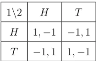
Another aspect that stresses the asymptotic nature of Theorem 2 is that it requires a class of payoff functions for which an equilibrium is sure to exist whenever the game has a continuum of players. In particular, it is false for games in which players have general payoff functions. As a simple example, consider ε = 1/4, and the following games Gn with X = {H, T }
and n ≥ 2: players 1 and 2 play the matching pennies (see Table 1), while the remaining players are indifferent between all strategies (i.e., Un(t)(f ) = 0
for all strategies f ).
1\2 H T
H 1, −1 −1, 1
T −1, 1 1, −1
Table 1: Payoff Function for the Matching Pennies
Then, if f is a pure strategy, it follows that at least one of players 1 and 2 is not 1/4 – optimizing. This implies that f cannot be a 1/4 – equilibrium. Therefore, Gn has no pure, 1/4 – equilibrium for all n ≥ 2.
5
Games based on the Averages of Individual
Choices
Khan and Sun (1999) also consider the case in which the action space is endowed with a linear structure and each player’s payoff depends only on his choice and on the average of players’ choices. In this section, we establish an existence result for this case, as well. In particular, we show that an approximate equilibrium exists in all equicontinuous, and sufficiently large games if
1. the action space is a weakly compact subset of a separable Banach space and the average is a Bochner integral,
2. the action space is a norm compact subset of a Banach space and the average is again a Bochner integral,
3. the action space is a weak* compact subset of the dual of a separable Banach space and the average is a Gel’fand integral and
4. the action space is a denumerable subset of R∞.
We emphasize that these results are obtained as corollaries of Theorem 2. Although a direct argument is possible, this highlights the additional generality of considering games in which each player’s payoff depends on the distribution of players’ choices when compared with games in which it depends only on the average of players’ choices.
5.1
Bochner Integral with the Weak Topology
In this subsection, assume that X is a weakly compact subset of a separable Banach space B. Let co(X) denote the closed convex hull of X, which is also weakly compact (see Diestel and Uhl (1977, Theorem 11, p. 51)). It follows from Dunford and Schwartz (1957, Theorem V.6.3, p. 434) that both X and co(X) are metrizable. Finally, let Uw be the space of weakly continuous
real-valued functions on X × co(X) endowed with the sup norm. If f : Tn → X is a pure strategy in a game with n players, let
R
Tnf dνn
denote its Bochner integral. Clearly, Z Tn f dνn= 1 n n X t=1 f (t) ∈ co(X).
In this case, we associate to each player t a weakly continuous function Vn(t) :
X × co(X) → R and define player t’s payoff function as Un(t)(f ) = Vn(t) µ f (t), Z Tn f dνn ¶ , (17)
for any strategy f : Tn→ X. We denote this class of games by Hw.
Corollary 1 Let K be an equicontinuous subset of Uw. Then, for all ε > 0
there exists N ∈ N such that n ≥ N and Vn(Tn) ⊆ K implies that Gn∈ Hw
has a pure ε – equilibrium.
5.2
Bochner Integral with the Norm Topology
In this subsection, assume that X is a norm compact of a Banach space B. Then, co(X) is also norm compact (see Diestel and Uhl (1977, Theorem 12, p. 51)). We let Unorm be the space of norm continuous real-valued functions
Finally, we let Hnorm be the class of games defined as in Subsection 5.1,
except that now players’ payoff functions belong to Unorm (and X is norm
compact).
As in Khan, Rath, and Sun (1997), Corollary 1 also applies to the case of norm compact action spaces. Note that X is weakly compact. Thus, since norm continuous functions on norm compact sets are weakly continuous, we obtain the following existence result.
Corollary 2 Let K be an equicontinuous subset of Unorm. Then, for all
ε > 0 there exists N ∈ N such that n ≥ N and Vn(Tn) ⊆ K implies that
Gn ∈ Hnorm has a pure ε – equilibrium.
5.3
Gel’fand Integral
In this subsection, let B∗ be the dual of a separable Banach space B and
assume that X is a weak* compact subset of B∗. Then, co(X) is also weak*
compact. It follows from Rudin (1971, Theorem 3.16, p. 70) that both X and co(X) are metrizable. Finally, let Ug be the space of weak* continuous
real-valued functions on X × co(X) endowed with the sup norm. If f : Tn → X is a pure strategy in a game with n players, let
R
Tnf dνn
denote its Gel’fand integral. Clearly, Z Tn f dνn= 1 n n X t=1 f (t) ∈ co(X).
We associate to each player t a weak* continuous function Vn(t) : X ×
co(X) → R and define player t’s payoff function as
Un(t)(f ) = Vn(t) µ f (t), Z Tn f dνn ¶ , (18)
for any strategy f : Tn→ X. We denote this class of games by Hg.
Corollary 3 Let K be an equicontinuous subset of Ug. Then, for all ε > 0
there exists N ∈ N such that n ≥ N and Vn(Tn) ⊆ K implies that Gn ∈ Hg
has a pure ε – equilibrium.
5.4
Games with Denumerably Many Actions in R
∞In this subsection, we consider the class of games defined in Section 5 of Khan, Rath, and Sun (1997). Let R∞ be the space of all real sequences
equipped with the product topology. The standard basis vectors are denoted by {ei}∞i=1. We let the space of actions be X = {ei}∞i=0 with e0 ≡ 0. Again,
co(X) denotes the closed convex hull of X, which is equal to the set of all sequences of real numbers chosen from the closed unit interval. Finally, let
U∞ be the space of continuous real-valued functions on X × co(X) endowed
with the sup norm.
The following definitions are from Khan, Rath, and Sun (1997). If (T, T , ν) is a probability space, then a function f : T → R∞is measurable if f−1({e
i}) ∈ T . In this case, Z T f dν = ∞ X i=1 eiν(f−1({ei})).
In particular, if µ ∈ M(X), thenRX idµ =P∞i=1eiµ({ei}) and so we trivially
obtain the following change of variable formula: Z T f dν = Z X idν ◦ f−1.
Furthermore, if j ∈ N and πj : R∞ → R is the projection onto the jth
coordinate, then πj is a simple function and its Lebesgue integral is
R
X πjdµ =
If f : Tn→ X is a pure strategy in a game with n players, then, clearly, Z Tn f dνn= 1 n n X t=1 f (t) ∈ co(X).
In this case, we associate to each player t a continuous function Vn(t) :
X × co(X) → R and define player t’s payoff function as Un(t)(f ) = Vn(t) µ f (t), Z Tn f dνn ¶ , (19)
for any strategy f . We denote this class of games by H∞.
Corollary 4 Let K be an equicontinuous subset of U∞. Then, for all ε > 0
there exists N ∈ N such that n ≥ N and Vn(Tn) ⊆ K implies that Gn∈ H∞
has a pure ε – equilibrium.
6
Mixed Strategies
In this section, we allow players to choose mixed strategies. In this context, a mixed strategy for a player is a Borel probability measure on the set of his pure strategies. Thus, a mixed strategy is a function f : Tn→ M(X), while
a pure strategy is a function g : Tn → X. Note that a pure strategy can
be seen as a mixed strategy, simply by associating X with the degenerate probability measures on X.
Given a strategy f in a game with n players, the distribution of players’ choices is νn◦ f−1, now an element of M(M(X)). Consequently, players’
payoff functions are elements of Um, which we use to denote the space of all
As in Section 2, we associate to each player a function Vn(t) : X ×
M(M(X)) → R with the following interpretation: Vn(t)(x, µ) is player t’s
payoff when he plays action x and facing the distribution µ. Then, for any strategy f , player t’s payoff function is
Un(t)(f ) =
Z
X
Vn(t)(x, νn◦ f−1)dft(x). (20)
We let Hm denote this class of games.
Since M(X) is (homeomorphic to) a closed subset of M(M(X)), then each game Gn in which mixed strategies are allowed induces a game ˜Gn in H
simply by restricting players’ payoff functions to X × M(X). Furthermore, if K ⊆ Um is equicontinuous, then ˜K ⊆ U defined by restricting the domain
in this way is also equicontinuous. Thus, for all K ⊆ Um and all ε > 0, if n is
sufficiently large, then ˜Gn has a pure strategy ε/3 – equilibrium f : Tn→ X.
It is easy to see that f is also an ε – equilibrium of Gn since for every t ∈ Tn
and ˜ft∈ M(X), Vn(t)(f (t), νn◦ f−1) ≥ Z X Vn(t)(x, νn◦ f−1)d ˜ft(x) − 2ε 3 ≥ Z X Vn(t)(x, νn◦ (f \tf˜t)−1)d ˜ft(x) − ε. (21)
Note that both inequalities hold since Vn(Tn) is a subset of an equicontinuous
family in Um and if n is sufficiently large to imply that the change from
νn◦ (f \tx)−1 to νn◦ f−1 and from νn◦ f−1 to νn◦ (f \tf˜t)−1, respectively,
produces at most a change of ε/3 in players’ payoffs. Thus, we obtain the following existence result.
Theorem 5 Let K be an equicontinuous subset of Um. Then, for all ε > 0
there exists N ∈ N such that n ≥ N and Vn(Tn) ⊆ K imply that Gn ∈ Hm
An interesting question that arises once we consider mixed strategy is if all Nash equilibria can be approximately purified. In Carmona (2005a), we show that the answer is no.
7
On the Need for Equicontinuity
In this section, we show that in general, we cannot obtain a pure strategy Nash equilibrium even in equicontinuous large games. The exact version of Theorem 2 (i.e., with ε = 0) therefore holds only in the limit case of games with a continuum of players. As an easy consequence, we also show that it is not possible to dispense with the equicontinuity assumption used in Theorem 2.
The idea of the example is simple: each player has two actions, zero or one, to choose from. Player 1 wants to mismatch the average (if everyone else chooses 1, he prefers 0, and vice versa), while player 2 wants to match. For half of the remaining players, 0 is the dominant strategy, while 1 is the dominant strategy for the other half. This last condition forces the average to close to 1/2 and pins down the behavior of all the players, except for players 1 and 2. At this point, we are in a matching pennies situation: if a strategy prescribes different actions for them, then player 2 would like to deviate to match player 1’s choice; if a strategy prescribes the same action for both of them, then player 1 would like to deviate to mismatch player 2’s choice. Hence, no pure equilibrium can exist.
Here are the details. Let n ≥ 4 be even. Let Tn = {1, . . . , n} be
|Tn,3| = |Tn,4| = n/2 − 1.
Let X = {0, 1}. Let i : X → X be the identity function, νn be the
uniform measure on Tn and µ ∈ M(X).
Let αn= 1 (below, we will change it). Define payoff functions as follows:
Vn(1)(x, µ) = αn(−1)x µZ X idµ − 1 2 ¶ . (22)
For player 2, define Vn(2)(x, µ) = −Vn(1)(x, µ).
Define W3(x, µ) = 10 if x = 1 0 if x = 0. (23)
and W4 = −W3. For a player t ∈ T3, let Vn(t) = W3, while for a player t ∈ T4
let Vn(t) = W4.
Let Gn be as defined above whenever n ≥ 4 is even. In the other case,
define Gn by setting Vn(t) = V3 for all t ∈ Tn.
Note that if f : Tn→ X is a strategy then
Z X idνn◦ f−1 = n X t=1 f (t) n .
We claim that if n ≥ 4 is even, then Gn has no pure strategy Nash
rium. We prove the above claim by contradiction. Let f be a Nash equilib-rium. Then, f (t) = 1 if t ∈ T3 0 if t ∈ T4. (24) Regarding f (1) and f (2), we consider the four possible cases.
Case 1 is when f (1) = 1 and f (2) = 0. In this case,
n X t=1 f (t) n = 1 2
and n X t=1 (f \21)(t) n = 1 2+ 1 n. Therefore, Vn(2)(f (2), νn◦f−1) = 0 and Vn(2)(1, νn◦(f \21)−1) = αn ¡1 2 +n1 − 12 ¢ . Hence, Vn(2)(1, νn◦ (f \21)−1) − Vn(2)(f (2), νn◦ f−1) = αn n = 1 n > 0, (25) a contradiction.
Case 2 is when f (1) = 0 and f (2) = 1. Then, Pnt=1f (t)n = 1 2 and Pn t=1 (f \20)(t) n = 1 2 − 1 n. Therefore, Vn(2)(0, νn◦ (f \20)−1) − Vn(2)(f (2), νn◦ f−1) = αn n = n1 > 0, a contradiction.
Case 3 is when f (1) = f (2) = 0. In this case,Pnt=1 f (t)n = n/2−1n = 1 2 − 1 n and Pnt=1(f \11)(t) n = 12. Therefore, Vn(1)(1, νn◦ (f \1 1)−1) − Vn(1)(f (1), νn◦ f−1) = αn n = 1 n > 0, a contradiction.
Finally, we consider the case f (1) = f (2) = 1. In this case, Pnt=1 f (t)n =
n/2−1+2 n = 1 2 + 1 n and Pn t=1 (f \10)(t) n = 1 2. Therefore, Vn(1)(0, νn◦ (f \10)−1) −
Vn(1)(f (1), νn◦ f−1) = αnn = n1 > 0, a contradiction. This proves the claim.
Note that the family of payoff functions used, which equals
{V1(1), V1(2), W3, W4},
is equicontinuous. But, despite this, we cannot guarantee the existence of a pure strategy Nash equilibrium, even if n is large.
This example can be easily modified to show that the conclusion of Theo-rem 2 fails, if we drop the equicontinuity assumption. Simply define αn= 2n,
n ≥ 4 is even, then Gn has no pure 1 – equilibrium.2
Note that, in this case, the family of payoff functions is equal to
{V3, V4}
[
∪∞
n=1{Vn(1), Vn(2)}.
Since limn→∞αn= ∞, it follows that it is not equicontinuous. This accounts
for the failure of the conclusion of Theorem 2.
8
Relation with Khan and Sun (1999)
Khan and Sun (1999) stated an asymptotic existence theorem for large games based on non-standard methods. For the class of games we consider here, they state the following result: Let {Gn}∞n=1 ⊆ H be a tight sequence of
games (i.e., the sequence {νn ◦ Vn−1}∞n=1 ⊆ M(U) is tight). Then, for all
ε > 0 there exists N ∈ N such that for all n ≥ N there exists f : Tn → X
such that for all t ∈ Tn and all x ∈ X,
Vn(t)(f (t), νn◦ f−1) ≥ Vn(t)(x, νn◦ f−1) − ε. (26)
However, we can modify the example presented in Section 7 to show that this statement is false.3
2Again, we assume that a 1 – equilibrium exists. Then, players in T
3 must play 1 and
players in T4 must play 0. We then consider the four possible case for players 1 and 2.
The above formulas show that there is at least one player whose gain from deviation is
αn/n = 2 > 1, which is a contradiction.
3The reason we need to modify the example is that our equilibrium notion is different
than theirs. Theirs assumes that a player’s deviation does not affect the distribution of actions. Note that the family of payoff functions used in our second example in Section 7 (i.e., when αn= 2n) is tight, and so it also shows that the above conclusion fails for our equilibrium concept.
The difficulty with the statement in Khan and Sun (1999) is that there is a small fraction of players whose payoff function might be extremely sensitive to small changes in the distribution of choices. Thus, we cannot guarantee that those players are almost optimizing.
This suggests that their result is valid if we define approximate equilibria by requiring that a large fraction of players is almost optimizing. Formally, for all ε, η ≥ 0, a strategy f is an (ε, η) – equilibrium of Gn if
|{t ∈ Tn : Un(t)(f ) ≥ Un(t)(f \tx) − ε for all x ∈ X}|
n ≥ 1 − η. (27)
Regarding this notion, we obtain the following existence result.4
Theorem 6 Let Γ ⊆ H be a tight family of games. Then, for all ε > 0 and
η > 0 there exists N ∈ N such that n ≥ N and implies that Gn ∈ Γ has a
pure (ε, η) – equilibrium.
This is the correct statement of Kahn and Sun’s result, which was also pointed out by Sun (2005). This result is, however, equivalent to our Theorem 2.5
Theorem 7 Theorem 2 holds if and only if Theorem 6 holds.
Of course, this implies that Kahn and Sun’s theorem is also equivalent to Mas-Colell’s. In fact, this is how we prove the above result: it is easier to compare both our Theorem 2 and Kahn and Sun’s with Mas-Colell’s than to compare them directly. As is typically the case, non-atomic games are easier to study and are, therefore, useful even when one is only interested in large finite games.
4Its proof is a simple variation of that of Theorem 2 and is presented in Appendix A.4. 5Its proof is a simple variation of that of Theorem 4 and is presented in Appendix A.5.
9
Concluding Remarks
The main objective of this paper is to argue for Mas-Colell’s formalization of the equilibrium theory of large games in terms of distributions. We follow his approach and show that:
1. for any equicontinuous family of payoff functions and any ε > 0, all sufficiently large games have a pure ε – equilibrium;
2. the above asymptotic result is equivalent to Mas-Colell’s and 3. it is also equivalent to Khan and Sun’s.
Therefore, we can construct an equilibrium theory of large finite games using Mas-Colell’s model, which is as rich as the one developed by Kahn and Sun (and as rich as the theory obtained by Mas-Colell for games with a continuum of players). To put it differently, the existence of pure strategy Nash equilibria in games with a continuum of players can be studied equivalently to the existence of pure approximate equilibria in large, equicontinuous games.
These results provide an additional example of the type of results showing that approximate equilibria of finite games have the same, or approximately the same, properties as equilibria of continuum games. In this way, it stresses the close relationship between equilibria of games with a continuum of players and approximate equilibria of games with a finite number of players.
A
Appendix
A.1
Lemmata
In this appendix, we prove several results needed for our main results. Lemma 1 deals with measures with a finite support, which can be thought of as a vector in some Euclidean space. Roughly, Lemma 1 says that the Prohorov distance between two measures whose support is contained in some finite set is proportional to their Euclidean distance.
Lemma 1 Let τ, µ ∈ M(X) be such that supp(τ ) ∪ supp(µ) ⊆ Ψ, where Ψ
is a finite set. If there exists ε > 0 such that |τl− µl| ≤ ε for all 1 ≤ l ≤ |Ψ|,
then ρ(τ, µ) ≤ |Ψ|ε.
Proof. Let ε > 0 and B ⊆ X be Borel measurable. Then,
τ (B) = X l∈Ψ∩B τl ≤ X l∈Ψ∩B (µl+ ε) ≤ X l∈Ψ∩B µl+ |Ψ|ε ≤ µ(B|Ψ|ε(B)) + |Ψ|ε. (28)
Similarly, we can show that µ(B) ≤ τ (B|Ψ|ε(B)) + |Ψ|ε. This implies that
ρ(τ, µ) ≤ |Ψ|ε.
Lemma 2 shows that in large games, deviations by a small fraction of players have a small impact on the distribution of actions.
Lemma 2 Let Gn∈ H be a game and let f and g be strategies. If
|{t ∈ Tn : f (t) 6= g(t)}|
then
ρ(νn◦ f−1, νn◦ g−1) ≤ γ. (30)
Proof. Let µ = νn ◦ f−1 and τ = νn ◦ g−1. Let B ⊆ X be Borel
measurable. Then, τ (B) = |{t : g(t) ∈ B}| n ≤ |{t : f (t) ∈ B}| n + |{t : f (t) 6= g(t)}| n = µ(B) + |{t : f (t) 6= g(t)}| n ≤ µ(Bγ(B)) + γ. (31)
Similarly, we can show that µ(B) ≤ τ (Bγ(B))+γ. This implies that ρ(τ, µ) ≤
γ.
In particular, we have that ρ(νn◦f−1, νn◦(f \tx)−1) ≤ 1/n for all strategies
f , players t ∈ Tn and actions x ∈ X.
Lemma 3 establishes the existence of an approximate equilibrium distri-bution with finite support for games with finitely many characteristics. Lemma 3 Suppose that µ ∈ M(U) has finite support and let τ be an
equi-librium distribution of µ. Then, there exists a sequence {τk}∞k=1 ⊆ M(U ×X)
such that
1. τk converges to τ ,
2. τU,k = µ for all k,
3. τX,k has finite support for all k,
5. for all ε > 0, there exists K ∈ N such that
τk({(u, x) : u(x, τX,k) ≥ u(X, τX,k) − ε}) = 1,
for all k ≥ K.
Proof. Let supp(µ) = {u1, . . . , un}. Letting Di = {x ∈ X : (ui, x) ∈
supp(τ )} for all 1 ≤ i ≤ n, the fact that τU = µ readily implies that
supp(τ ) = ∪n
i=1({ui} × Di). This follows because supp(τ ) ⊆ ∪ni=1({ui} × X)
since ∪n
i=1({ui} × X) is closed and τ (∪ni=1({ui} × X)) =
Pn
i=1τU({ui}) = 1.
For all 1 ≤ i ≤ n, define ci = µ({ui}) and
τi(B) = τ ({ui} × B)/ci
for all Borel subsets B of X. For latter use, we claim that supp(τ ) = ∪n
i=1({ui} × supp(τi)) .
Since ∪n
i=1({ui} × supp(τi)) is closed and
τ (∪n
i=1({ui} × supp(τi))) =
X i τ ({ui} × supp(τi)) = X i ciτi(supp(τi)) = 1,
it follows that supp(τ ) ⊆ ∪n
i=1({ui} × supp(τi)). Conversely, recall that
supp(τ ) = ∪n
i=1{ui} × Di. Since supp(τ ) is closed, one easily sees that Di is
closed. Furthermore,Pni=1τ ({ui}×Di) = τ (supp(τ )) = 1 and τ ({ui}×Di) ≤
τ ({ui}×X) = ci imply that τ ({ui}×Di) = ci, that is, τi(Di) = 1. Therefore,
supp(τi) ⊆ Di and so, {ui} × supp(τi) ⊆ {ui} × Di. Finally, one obtains that
∪n
i=1({ui} × supp(τi)) ⊆ ∪ni=1({ui} × Di) = supp(τ ).
The measure τi can be thought of as a measure in supp(τi), a closed
such that supp(τi,k) is a finite subset of supp(τi) and τi,k converges to τi in
supp(τi). Since supp(τi) is closed in X, then, by Lemma 6, we have that τi,k
converges to τi in X.
Let C be a Borel measurable subset of U × X. Then, let Bi = {x ∈ X :
(ui, x) ∈ C} and define τk(C) = n X i=1 ciτi,k(Bi).
Note that τU,k({ui}) = ci for all 1 ≤ i ≤ n and so τU,k = µ for all k.
Also, it is clear that τX,k has finite support for all k. Furthermore, since
τk({(ui, x)}) = ciτi,k({x}) and so τk({(ui, x)}) > 0 if and only if τi,k({x}) > 0,
it follows that
supp(τk) = ∪ni=1({ui} × supp(τi,k)) .
This immediatly implies that supp(τk) ⊆ supp(τ ) for all k, since supp(τi,k) ⊆
supp(τi).
We claim that τk converges to τ . This follows since, if h : U × X → R is
continuous and bounded, then x 7→ h(ui, x) is also continuous and bounded
for all 1 ≤ i ≤ n, and so Z U×X hdτk = n X i=1 Z {ui}×X hdτk = n X i=1 Z X h(ui, x)dτi,k(x) → n X i=1 Z X h(ui, x)dτi(x) = Z U×X hdτ.
We finally establish property 5. For convenience, for all η ≥ 0 and σ ∈
M(U × X), let Bη
σ = {(u, x) ∈ U × X : u(x, σX) ≥ u(X, σX) − η}, and
Bσ = Bσ0 if η = 0. Let ε > 0. Since Bτ is closed and τ (Bτ) = 1, then
Let δ > 0 be such that max{d(x, y), ρ(µ, ν)} < δ implies that |u(x, µ) −
u(y, ν)| < ε/2 for all u ∈ {u1, . . . , un}.
Let K ∈ N be such that ρ(τX,k, τX) < δ for all k ≥ K. Then, supp(τk) ∩
Bτ ⊆ supp(τk) ∩ Bετk, since if (u, x) ∈ supp(τk) ∩ Bτ and y ∈ X then
u(x, τX,k) > u(x, τX) − ε/2 ≥ u(y, τX) − ε/2 > u(y, τX,k) − ε since u ∈
{u1, . . . , un}. So
τk(Bτεk) = τk(supp(τk) ∩ B
ε
τk) ≥ τk(supp(τk) ∩ Bτ) = τk(supp(τk)) = 1. (32)
This concludes the proof.
Lemma 4 strengthens the conclusion of Lemma 3, whenever the set of players’ characteristics is a finite subset of an equicontinuous family. It guar-antees the existence of a finite set of actions with the property that all the above games have an approximate equilibrium strategy taking values in this finite set. The strength of this result is that the finite set works uniformly for all such games, i.e., it depends only on the equicontinuous set and on the degree of approximation desired.
Lemma 4 Let K be an equicontinuous subset of U. Then, for all η > 0,
there exists {x1, . . . , xm} ⊆ X such that the following holds:
1. X = ∪m
i=1Bη(xi) and
2. if G = (([0, 1], λ), V, X) is such that V ([0, 1]) is finite, then there exists a strategy g such that g([0, 1]) ⊆ {x1, . . . , xm} and
V (t)(g(t), λ ◦ g−1) > V (t)(X, λ ◦ g−1) − η
Consequently, if V ([0, 1]) is a subset of K, then g is an η – equilibrium.
Proof. Let η > 0. Since K is equicontinuous, there exists δ > 0 such that max{d(x, y), ρ(µ, ν)} < δ implies that |u(x, µ) − u(y, ν)| < η/3 for all
x, y ∈ X, µ, ν ∈ M(X) and u ∈ K. We can choose δ < η.
Let {x1, . . . , xm} be such that X = ∪mj=1Bδ/2(xj). Define B1 = Bδ/2(x1)
and Bj = Bδ/2(xj) \
¡
∪jl=1Bδ/2(xl)
¢
, 2 ≤ j ≤ m.
Let G be such that V ([0, 1]) is a finite subset of U. By Mas-Colell Theo-rem, G has an equilibrium distribution. It follows from Lemma 3 that G has an η/3 – equilibrium distribution with finite support and so a pure strategy
η/3 – equilibrium f (this follows easily from Liaponov’s Theorem (see Rudin
(1971, Theorem 5.5, p. 120))).
Define g : [0, 1] → {x1, . . . , xm} by g(t) = xj if f (t) ∈ Bj. Then, clearly
|f (t) − g(t)| < δ/2. This implies that
{t ∈ [0, 1] : g(t) ∈ D} ⊆ {t ∈ [0, 1] : f (t) ∈ Bδ/2(D)}
for all Borel measurable subsets D of X and so
λ ◦ g−1(D) ≤ λ ◦ f−1(Bδ/2(D)) + δ/2.
Similarly, one can show that λ ◦ f−1(D) ≤ λ ◦ g−1(B
δ/2(D)) + δ/2. Thus,
ρ(λ ◦ g−1, λ ◦ f−1) ≤ δ/2. This implies that for all t ∈ V−1(K) and all x ∈ X,
V (t)(g(t), λ ◦ g−1) > V (t)(f (t), λ ◦ f−1) − η 3 ≥ V (t)(x, λ ◦ f−1) −2η 3 > V (t)(x, λ ◦ g−1) − η. (33)
In particular, if V ([0, 1]) ⊆ K, then g is an η – equilibrium of G.
Lemma 5 is used to draw conclusions for games with a continuum of players from properties of large finite games. It uses the definition of (ε, η) – equilibrium, given in Section 8. Furthermore, it considers a more general case in which a game Gn = ((Tn, νn), Vn, X) with finitely many players has
|Tn| players (not necessarily equal to n), and νn is the uniform measure on
Tn.
Lemma 5 Let G = (([0, 1], λ), V, X) be a game with a continuum of players,
τ be a distribution on U × X satisfying τU = λ ◦ V−1 and ε ≥ 0. Suppose that
{Gn}∞n=1 is a sequence of games with a finite number of players and {fn}∞n=1
is a sequence of strategies satisfying: 1. |Tn| → ∞,
2. fn is an (εn, ηn) – equilibrium of Gn,
3. εn ≥ ε, εn→ ε,
4. ηn≥ 0, ηn → 0 and
5. νn◦ (Vn, fn)−1 converges to τ ,
then τ is an ε – equilibrium distribution of G.
Lemma 5 is slightly more general than the sufficiency part of Theorem 1 in Carmona (2004). We include its proof for the sake of completeness.
Proof. Let τn= νn◦ (Vn, fn)−1. For all x ∈ supp(τn,X) and y ∈ X, define
τn,Xx,y as follows: τn,Xx,y(x) = τn,X(x) − 1/|Tn|, τn,Xx,y(y) = τn,X(y) + 1/|Tn| and
from y. Let Bεn
τn = {(u, x) ∈ supp(τn) : u(x, τn,X) ≥ u(y, τ
x,y
n,X)−εn for all y ∈
X}. Also, let Bε
τ = {(u, x) ∈ U × X : u(x, τX) ≥ u(X, τX) − ε}.
Since τn converges to τ , then τX,n converges to τX. Taking a subsequence
if necessary, we can assume that |Tn| % ∞, ρ(τX, τX,n) & 0, εn & ε and
ηn & 0. Let θn = ρ(τX, τX,n) + 2/|Tn|; clearly, θn & 0. Since, for all
x ∈ supp(τn,X) and y ∈ X, ρ(τX, τn,Xx,y) ≤ ρ(τX, τX,n) + ρ(τn,X, τn,Xx,y) ≤ ρ(τX, τX,n) + 1 |Tn| , (34)
it follows that ρ(τX, τn,Xx,y) < θn.
Define, for each u ∈ U,
βn(u) = sup x∈X,ν∈M(X)
{|u(x, ν) − u(x, τX)| : ρ(ν, τX) < θn}.
Since u is continuous on X × M(X), which is compact, it follows that u is uniformly continuous. Thus, βn(u) & 0 as n → ∞. We claim that βn is
continuous in U.
Let η > 0. Define δ < η/2. Then if ||u − v|| = supy∈X,φ∈M(X)|u(y, φ) − v(y, φ)| < δ, we have for any x ∈ X, and ν ∈ M(X) such that ρ(ν, τX) < θn
|v(x, ν) − v(x, τX)| ≤ |v(x, ν) − u(x, ν)| + |u(x, ν) + u(x, τX)|+
+ |v(x, τX) − u(x, τX)| < δ + βn(u) + δ,
(35)
and so βn(v) ≤ 2δ + βn(u) < η + βn(u). By symmetry, βn(u) < η + βn(v),
and so |βn(u) − βn(v)| < η. Hence, βn is continuous, as claimed.
Given the definition of βn, we have that Bτεnn ⊆ Dn := {(u, x) ∈ U × X :
u(x, τX) ≥ u(X, τX) − εn− 2βn(u)}. Since βn is continuous, we see that Dn
Let n ∈ N be given. Then, if k ≥ n, it follows that τk(Dn) ≥ τk(Dk) ≥ 1−
ηk ≥ 1−ηn, and so τ (Dn) ≥ lim supjτj(Dn) ≥ 1−ηnby Parthasarathy (1967,
II.6.1(c)). Hence, τ (Bε
τ) = limnτ (Dn) = 1. Therefore, τ is an equilibrium
distribution of G.
The following lemma shows that the convergence of a sequence of mea-sures can be studied with respect to any closed set containing both their support and the support of the limit measure.
Lemma 6 Let X be a metric space and µ, µn ∈ M(X) for all n ∈ N. Let C
be a closed subset of X satisfying supp(µn), supp(µ) ⊆ C. Then, µn ⇒ µ in
C if and only if µn ⇒ µ in X.
Proof. (Necessity) Let h : X → R be bounded and continuous. Then
h|C is also bounded and continuous, and so
Z C hdµn → Z C hdµ. Thus, Z X hdµn = Z C hdµn → Z C hdµ = Z X hdµ. It follows that µn⇒ µ in X.
(Sufficiency) Let h : C → R be bounded and continuous. Then by the Tietze-Urysohn extension theorem, there exists a bounded, continuous func-tion h∗ : X → R such that h∗(x) = h(x) for all x ∈ C. Therefore,
Z X h∗dµ n → Z X h∗dµ, and Z X h∗dµ = Z C h∗dµ = Z C hdµ
(and similarly, RXh∗dµ n =
R
Chdµn for all n ∈ N). Therefore,
R
Chdµn →
R
Chdµ. It follows that µn⇒ µ in C.
A.2
Proof of Corollaries 1, 3 and 4
The proof of each corollary follows the same idea. Hence, we will present it only for the case of Corollary 1.
Let ε > 0. Let V ∈ K and i : X → X denote the identity function in X. Define v : X × M(X) → R by v(x, µ) = V µ x, Z X idµ 
for all x ∈ X and µ ∈ M(X).
Note that i is Bochner integrable andRX idµ ∈ co(X) for all µ ∈ M(X).
Furthermore, if µk converges to µ, then
R
Xidµk converges weakly to
R
Xidµ
and so v is continuous.
Let g : X × M(X) → X × co(X) be defined by g(x, µ) = (x,RXidµ). In
order to apply Theorem 2, it remains to show that ˜K defined by {u ∈ U : u = v ◦ g for some v ∈ K} is equicontinuous.
Let d denote the metric in co(X). Let ε > 0 and let δ > 0 be such that
|v(x, z) − v(y, w)| < ε whenever max{d(x, y), d(z, w)} < δ and v ∈ K.
Note that it is enough to show that there exists η > 0 such that ρ(µ, τ ) < η implies d(RXidµ,RXidτ ) < δ.
Suppose, in order to reach a contradiction, that such η > 0 does not exist. Then, for all k ∈ N there are {µk} and {τk} such that ρ(µk, τk) < 1/k and
d(RXidµk,
R
Xidτk) ≥ δ. Since M(X) is compact, we may assume that there
R
Xidµkand
R
Xidτkconverge weakly to
R Xidµ. Hence, d( R Xidµk, R Xidτk) → 0, which is a contradiction.
Thus, ˜K is an equicontinuous subset of U. By Theorem 2, let N ∈ N be
such that n ≥ N implies that all games ˜Gn ∈ H with ˜V (Tn) ⊆ ˜K have an ε
– equilibrium.
Let n ≥ N and Gn ∈ Hw be such that V (Tn) ⊆ K. Define ˜Gn ∈ H by
letting ˜Vt = Vt◦ g. Then, ˜V (Tn) ⊆ ˜K and so there exists an ε – equilibrium
f : Tn→ X. Thus,
˜
Vt(f (t), νn◦ f−1) ≥ ˜V (x, νn◦ (f \tx)−1) − ε
for all t ∈ Tn and x ∈ X.
Note that ˜ Vt(f (t), νn◦ f−1) = Vt◦ g(f (t), νn◦ f−1) = Vt µ f (t), Z X idνn◦ f−1 ¶ , ˜ Vt(x, νn◦ (f \tx)−1) = Vt µ x, Z X idνn◦ (f \tx)−1 ¶ , Z X idνn◦ f−1 = 1 n n X t=1 f (t) = Z Tn f dνn and Z X idνn◦ (f \tx)−1 = 1 n n X ˜ t=1 (f \tx)(˜t) = Z Tn (f \tx)dνn. Therefore, Vt µ f (t), Z Tn f dνn ¶ ≥ Vt µ x, Z Tn (f \tx)dνn ¶ − ε, (36) and so f is an ε – equilibrium of Gn.
A.3
Example for Section 8
Let n ≥ 4 be even. Let Tn = {1, . . . , n} be partitioned into four sets: Tn,1=
{1}, Tn,2= {2}, Tn,3 and Tn,4 satisfying |Tn,3| = |Tn,4| = n/2 − 1.
Let X = {0, 1}. Let i : X → X be the identity function, νn be the
uniform measure on Tn and µ ∈ M(X).
Let γ > 1, 1 1 + 2/n < βn< 1 and αn = max ½ 2 βn+ 2βn/n − 1 , 2 1 − βn+ 2βn/n , 2 1 − βn ¾ . (37)
Clearly, αn> 0. In fact, αn→ ∞ since βn→ 1.
Define payoff functions as follows:
Vn(1)(x, µ) = αn(−1)x µ βn Z X idµ − 1 2 ¶ . (38)
For player 2, define
W2(x, µ) = 2 γ − 1(−1) x µ 1 2− γ Z X idµ ¶ . (39) and Vn(2) = W2. Define W3(x, µ) = 10 if x = 1 0 if x = 0. (40)
and W4 = −W3. For a player t ∈ T3, let Vn(t) = W3, while for a player t ∈ T4
let Vn(t) = W4.
Let Gn be as defined above whenever n ≥ 4 is even. In the other case,