BPI - Banco Português do Investimento : Equity Research

(1)

Universidade Católica Portuguesa

Catolica Lisbon School of Business & Economics

Banco Português do Investimento

Equity Research

Inês Guedes de Andrade Costa Simões, 152110062

Abstract

In the recent years, many valuation models have been developed, and the debate on how best to estimate a company’s value, which assumptions should be made and what are the most adequate approaches to apply is still ongoing. The purpose of this dissertation is to bring some clarity upon Equity Research, by combining a review of considerable academic literature with the valuation of Banco Português de Investimento. In the end, I will also do a comparison for both methodologies followed and results obtained by Caixa Banco de Investimento in their report published on the 12th December 2011.

Advisor: Prof. José Carlos Tudela Martins

Dissertation submitted in partial fulfillment of requirements for the degree of MSc in Business Administration, at the Universidade Católica Portuguesa, 4th January 2012.

(2)

i

3.1. Company Presentation ... 30 3.1.1. Shareholders Structure ... 31 3.1.2. Financial Indicators ... 31 3.1.3. Strategy... 38 3.2. Sector Analysis ... 39 3.2.1. Portugal... 39 3.2.2. Angola ... 41 3.2.3. Future prospects ... 46 3.3. Regulatory Framework ... 47 4. Valuation Methodology ... 50 5. Assumptions... 51 5.1. General Assumptions ... 51

5.2. Related with the discount rate ... 53

6. Valuation of BPI ... 56

6.1. Total credits and loans and Total resources... 56

6.2. Net Operating Income ... 58

6.2.1. Commissions ... 58

6.2.2. Net Interest Income ... 59

6.3. Operating Costs ... 62

7. Performance Evaluation ... 65

(4)

iii

7.2. Assets Quality ... 66

7.3. Pension Funds ... 68

8. Valuation Results ... 70

8.1. Dividend Discount Model ... 70

8.2. Residual Income ... 72

8.3. Equity Discount Model ... 74

8.4. DuPont ... 75

8.5. Relative Valuation ... 76

8.6. Final price target ... 78

8.7. Scenarios ... 79

8.7.1. Greek debt 100% haircut ... 79

8.7.2. Recapitalization ... 80

8.7.3. 100% Greek haircut and recapitalization ... 81

8.7.4. Merger/ Acquisition ... 81

9. Valuation Comparison with Caixa BI ... 83

10. Conclusion ... 87

11. Appendixes ... 88

(5)

iv

I. Preface

It is my objective on this dissertation to value Banco Português de Investimento, hereon referred as BPI, considered as the 4th major Portuguese private financial group, listed on the PSI-20 stock exchange. Through matching theory with practice and consequently by applying some valuation models, I will provide a recommendation on the FY12 stock price. The important and particular role banks have in the allocation of capital in the economic system, and the fact that a banks’ business model display some peculiarities, imply a special treatment in the approach to its valuation, being therefore more challenging, what had influenced me on my decision of what company to choose.

The structure of the thesis is as follows:

I start with a brief executive summary (Ch.1), which is followed by the literature review (Ch. 2), where, according to academic literature, I explain the role of valuation in economy, how to choose a valuation model and enumerate some of the most common approaches used as well as briefly explain how to apply them. Moreover, guidance for valuating financial services and cross border valuations is also presented in this chapter. Afterwards, on Ch.3, a company presentation is done, in which I cover some topics as the history of BPI, its major operations, shareholder structure, and present a number of performance indicators. An industry analysis and an overview over the regulatory framework in which financial services operate is also included in this chapter, in order to identify the key factors that drive this business as well as understanding the economic environment in which BPI is operating and the impacts it may have on BPI’s strategy. In Ch.4, the valuation methodology followed is described. The macroeconomic assumptions and the valuation drivers related with BPI’s accounts are on Ch. 5 and Ch. 6, respectively. On Ch. 7, some performance indicators are analyzed, such as the asset quality, and solvency to understand if, according to my estimates the bank would improve its position in the market and comply with the regulation or not. Finally, on Ch.8 the valuation results are disclosed, where I present the final price target recommendation, and on Ch.9 a comparison with Caixa BI methodology and results is done. To finish, on Ch. 10 the main conclusions of this dissertation are summarized.

(6)

v

II. Acknowledgments

In order to develop this dissertation, I had the opportunity to establish contact with a number of people that were important by the support and learning experience provided, having each one a specific role and contribution to the final output, to who I would like to express my gratitude:

First of all, I would like to appreciate the support that Dr. Gonçalo Vaz Botelho provided during my master, being always present and available to advice me. Besides, I would also like to thanks him the opportunity he gave me to incorporate the Equity Research team of Caixa Banco de Investimento, where I did my curricular internship, and which contributed significantly to the development of my thesis.

On Caixa BI, I am grateful to the support, expertise and invaluable knowledge transmitted by: Dr. João Miguel Lourenço, Dr. André Rodrigues, Guido Varatojo dos Santos, Dr. Helena Barbosa, and Dr. Carlos Jesus. With all of them, I took advantage of a very enrichment experience, where I had learned a lot, grew up as a person, and had also great moments of funny.

At last I would also like to express my thankfulness to Professor José Carlos Tudela Martins, for his availability and helpful feedback concerning my thesis improvement and development, as also to Dr. Ricardo Araújo, head of the BPI Investor Relations Department, for the additional data and explanations provided to my questions concerning BPI.

(7)

vi

III. List of abbreviations

1H11 – 1st half of 2011

9M11 – 9 months of 2011 1Q11 – 1st quarter of 2011 ATA – Average total Assets

BCI – Banco Comercial e de Investimentos BdP – Bank of Portugal

BFA – Banco Fomento Angola BNA – Banco Nacional Angola

BIS – Bank for International Settlements BPI – Banco Português de Investimento BS – Balance Sheet

CAGR – Compounded Annual Growth Rate CAPM – Capital Asset Pricing Model CAR – Capital Adequacy Ratio CCF – Capital Cash Flow CF – Cash Flow

CRP – Country Risk Premium DCF – Discounted Cash Flow DPR – Dividend Payout Ratio EBA – European Banking Authority ECB – European Central Bank ERP – Equity Risk Premium FCFE – Free Cash Flow to Equity FCFF – Free Cash Flow to the Firm FY11 – Final year of 2011

GDP – Growth Domestic Product IAS – International Accouting Standards

(8)

vii

IB – Investment bank

IMF – International Monetary Fund NAV – Net Assets Value

NI – Net Income

NII – Net Interest Income NIM – Net Interest Margin NPL – Nonperforming Loans PER – Price Earnings Ratio

PVts – Present Value of Tax Shields

P/B – Price to Book Value P/E – Price Earnings Ratio RIV – Residual Income Valuation ROE – Return on Equity

ROA – Return on Assets TV – Terminal Value

US – United States of America Vu – Unlevered Value

WACC – Weighted Average Cost of Capital YoY – Year-on-year growth rate

(9)

1

1. Executive Summary

January 2012

Banco BPI

BANKS Inês Simões BUY Recommendation

Share Price: EUR 0.48

Closing price as 04/01/12

Target Price: EUR 0.83

FY 2012

BPI and PSI-20

BPI PSI-20

Market Cap (EURm) 471.24

Current n of shares (m) 990

52 Wk high Price: EUR 1.34

09/02/2011

52 Wk low Price: EUR 0.381

11/11/2011

1 Yr total return -62,52% Beta vs PSI-20 1.16

Bloomberg. BPI PL Equity

COMPANY REPORT

“Extreme uncertainty and volatility related to further development of the euro zone crisis should remain” (André Rodrigues, Caixa BI)

Taking into consideration both the macroeconomic scenario, as also, the set of requirements defined in the Memorandum agreed with Troika, the main challenge in the following years to the sector is related with banks’ ability to adapt to the new regulatory framework, maintaining an adequate flow of funding to the real economy and consequently promote economic growth.

Main drivers:

 Recession environment until 2013 at best  Higher level of regulation

 Higher capital needs  Higher liquidity levels  Higher transparency

 Acceleration in the deleveraging process  Marked competition on the deposits side

 High levels of funding through ECB - The uncertainty and volatility that characterize the current market, have lead Portuguese banks to be incapable of fund their activity in the international wholesale markets

(10)

2

Banco BPI

BANKS

Inês Simões

Solvency

Over the last months BPI (as well as its peers), has been opting for the reinforcement of its balance sheet, what has been leading to lower levels of profitability (in example, ROE of 8,8% in 2009 and 2010, and 6.1% in the 9M11). This is done namely via less credit amounts granted, more restrictive conditions, via the increase of the deposits amounts (which has lead to an intensification of the competitive environment in the domestic market – increase of the spreads offered and higher pressure on NIM), or by the sale of non-core assets.

These measures are also expected to be maintained in the near future so that the confidence on the financial system is recovered and banks liquidity is improved as well as its profitability by starting to have access to the wholesale funding markets again, which are associated with higher returns, instead of resourcing so much on the ECB funds.

Moreover, I expect the negative outlook in the medium term to strongly be affected by the sovereign debt crisis which is spread all over Europe. BPI’s exposure on the FY2010 ascended to €4,5 bn ~ 11% of the total assets, with a potential loss of €1,39 bn during the first half of 2012.

Profitability

Like any other bank, BPI will take a hit in profitability terms, on almost all possible fronts. The incapacity of BPI and other Portuguese banks to access international wholesale, and the higher funding costs demanded on it have made deposit-capturing a top priority in commercial terms, due to both liquidity and profitability concerns. Credit-concession has been re-priced in order to pass these higher costs of funding to customers, and to account for the deterioration of customers’ credit profile (less trustful economy, higher nonperforming loans, and drop in collateral value, among other factors).

Looking at BPI’s presence internationally, the credit granting activity is expected to remain value-creating, despite the fact that competition in the Angolan banking industry is likely going to increase over time.

January 2012

(11)

Equity Research 2012

3

Banco BPI

BANKS

Inês Simões

Besides the negative impact the closure of the international wholesale market has on BPI’s margins, it has been increasing the reliance on ECB, creating an unsustainable environment in the long term.

Assets Quality

Besides the difficulties that the bank will have associated with its solvency and profitability, the evolution of assets quality will also be a relevant topic, namely due to the increasing trend of the nonperforming loans verified in the last months. Economic factors such as slower growth, higher unemployment rates, the increase in interest rates, will likely reduce the disposable income of Portuguese households, and thus, are reflected into rising NPLs, which weakens corporate sector and the all economy.

Therefore, I expected the assets quality to continue with a negative trend in 2012 as the nonperforming loans increasing tendency should continue, which would be translated into higher credit risks, higher provisioning efforts, and lower short/ midterm profitability for BPI.

International operations

While the pressure increases in profitability terms for BPI’s domestic operation, the future prospects of its international businesses are growing in importance, in which BFA seems to be the way out for the bank, given the contrasts between the Portuguese and the Angolan banking sector, and the European sluggish outlook. BPI’s Angolan operation represents the bulk of its exposure to international markets, and its most important growth prospect. As a consequence, it is foreseen that BPI will be really focused on the development of its Angolan operation (physically extending its business), which will certainly negatively affect its operational efficiency, but may very well create a competitive advantage if other banks do not follow up on their plans too.

January 2012

(12)

Equity Research 2012 4

Banco BPI

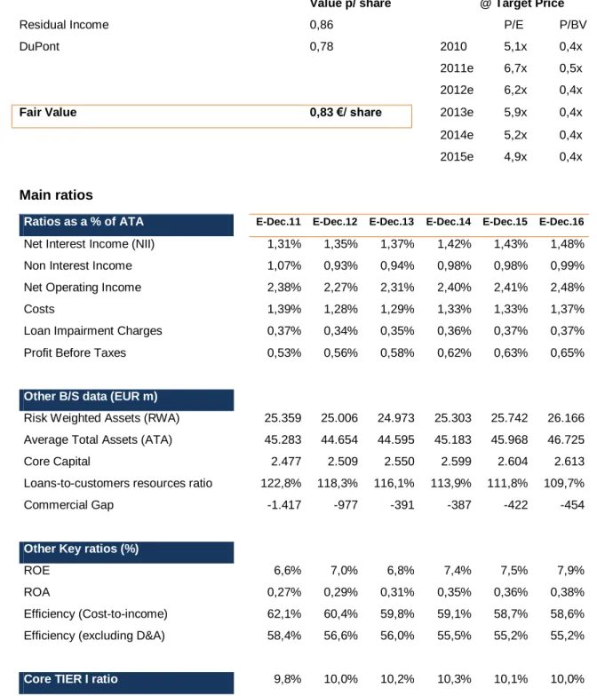
BANKS Inês Simões Valuation

BPI: Valuation Summary – Msc Thesis

Value p/ share @ Target Price

Residual Income 0,86 P/E P/BV

DuPont 0,78 2010 5,1x 0,4x

2011e 6,7x 0,5x

2012e 6,2x 0,4x

Fair Value 0,83 €/ share 2013e 5,9x 0,4x

2014e 5,2x 0,4x

2015e 4,9x 0,4x

Main ratios

Ratios as a % of ATA E-Dec.11 E-Dec.12 E-Dec.13 E-Dec.14 E-Dec.15 E-Dec.16

Net Interest Income (NII) 1,31% 1,35% 1,37% 1,42% 1,43% 1,48%

Non Interest Income 1,07% 0,93% 0,94% 0,98% 0,98% 0,99%

Net Operating Income 2,38% 2,27% 2,31% 2,40% 2,41% 2,48%

Costs 1,39% 1,28% 1,29% 1,33% 1,33% 1,37%

Loan Impairment Charges 0,37% 0,34% 0,35% 0,36% 0,37% 0,37%

Profit Before Taxes 0,53% 0,56% 0,58% 0,62% 0,63% 0,65%

Other B/S data (EUR m)

Risk Weighted Assets (RWA) 25.359 25.006 24.973 25.303 25.742 26.166 Average Total Assets (ATA) 45.283 44.654 44.595 45.183 45.968 46.725

Core Capital 2.477 2.509 2.550 2.599 2.604 2.613

Loans-to-customers resources ratio 122,8% 118,3% 116,1% 113,9% 111,8% 109,7%

Commercial Gap -1.417 -977 -391 -387 -422 -454

Other Key ratios (%)

ROE 6,6% 7,0% 6,8% 7,4% 7,5% 7,9%

ROA 0,27% 0,29% 0,31% 0,35% 0,36% 0,38%

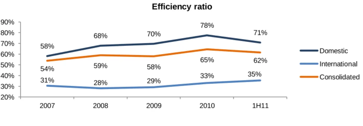
Efficiency (Cost-to-income) 62,1% 60,4% 59,8% 59,1% 58,7% 58,6%

Efficiency (excluding D&A) 58,4% 56,6% 56,0% 55,5% 55,2% 55,2%

Core TIER I ratio 9,8% 10,0% 10,2% 10,3% 10,1% 10,0% Figure 1 and 2. Msc Thesis Valuation summary and BPI main ratios

January 2012

(13)

5

2. Literature Review

2.1. The importance of valuation

The importance of valuation is reflected on many areas in finance, such as corporate finance, mergers and acquisitions and portfolio management.

In every business, the corporate finance objective is long-term shareholder value creation. If as Damodaran (2002) once stated, “Every asset, financial as well as real, has a value”, and we know how best to increase it by changing a firm’s investment, financing decisions and dividends policy, we will have the key to maximize a firm’s profits and reach its’ goals. Therefore, “understanding what determines a firm’s value, where does it come from, and knowing how to estimate it, is the prerequisite for making good decisions”, Damodaran

(2006).

Valuation also plays an important role when doing a merger or acquisition analysis, helping the bidding firm to decide which will be its bid, taking into account the target firm’s value, the synergy gains and also the restructuring and changing management costs.

Regarding portfolio management, valuation’s importance depends on an investor’s profile. If he or she is a passive investor, its role is meaningless, whereas if we talk about an active investor, valuation has a key role by providing information of what securities to select and how to build the optimal portfolio.

On this perspective, valuing companies and predicting stock prices and returns, can be considered as the holy grail of finance for investors. Market efficiency theory states that financial markets are efficient about prices, reflecting all the information available on the market, following this way a random walk. According to this theory, returns are unpredictable and therefore, “valuation methods appear as a support to help investors to analyze whether and why market prices deviate from value, and how quickly they revert back”, Damodaran (2006).

Summing up, company’s valuation is useful for firms to better understand what is the impact of their operational/ financing decisions, as well as macroeconomic factors on its’ value and consequently enable them to improve their performance in the market. Besides, it is also valuable for investors, helping them to improve their management decisions, maximizing their portfolio.

With this purpose, several empirical studies and valuation methods were developed, being the choice of which one to use dependent on the company’s operations and in which sector it operates in, among other factors. It is important to note that different approaches will

(14)

6 require different assumptions, and thus, the same values are not always achieved. However, if consistent assumptions are made these are expected to be similar.

2.2. Choosing a valuation model

Analysts facing the task of valuing a firm’s enterprise value or equity value, have to choose among several approaches, being each one, as mentioned on Goldman Sachs investment

research paper, All Roads Lead to Rome (1999), “no more than a particular way of

expressing the same underlying model, by making different aspects of valuation problem clearer in detriment of obscuring other aspects”.

The decision whether to choose a simple model or a more complex and sophisticated one, depends not only on the precision of the valuation that is required, as also, on the information level analysts have about the firm.

According to Damodaran (2002) there are three main categories. The first one, Discounted Cash Flow Valuation, discounts the present value of the expected cash flows at a rate that reflects its riskiness. The second, Relative Valuation, computes the value of a firm based on performance and accounting indicators of comparable firms. The last method, Contingent Claim Valuation is based on option pricing models and is used to value firms which have assets with options characteristics. Below there are the main valuation approaches which can be used within these three categories.

Discounted Cash Flow Valuation Relative Valuation Contingent Claim

Free Cash Flow Equity Cash Flow Capital Cash Flow Dividend Discount Model Adjusted Present Value Economic Profit

Dynamic ROE – DuPont approach

Price earnings ratio – PER Price to book ratio – P/B Price sales ratio – P/S

Enterprise value to EBITDA – EV/EBITDA

EV/EBIT (others)

Black and Scholes Binomial

Figure 3. Main Valuation Approaches

From the ones mentioned above, I will just cover the ones I believe that are most important and most used by practitioners.

(15)

7

2.3. Main Valuation Models

2.3.1. Discounted Cash Flow Valuation

As mentioned above, the discounted cash flow method relies on the premise that the value of a business depends on its future economic benefits, and therefore consists on attempting to estimate the intrinsic value of an asset based upon its expected cash flows, by considering that a firm is a function of three variables – capacity to generate CF, its expected growth rate and the risk/ uncertainty associated with them.

Where,

n = Life of the Asset

CFt = Cash Flow in Period t

r = Discount rate reflecting the riskiness of the estimated Cash Flows

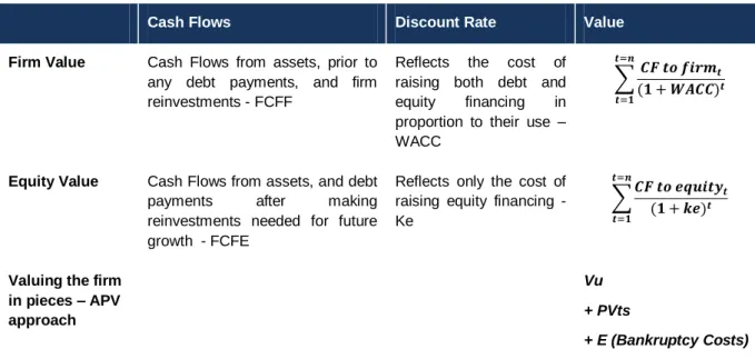
Under this formula and depending on the path we follow to value a company, based on equity, enterprise value, or on the value of the firm in pieces (APV approach), the expected cash flows and discount rate will change. It is expected to have higher discount rates to discount CF when dealing with riskier assets and lower discount rates for safer assets. (Damodaran 2002 and 2006)

Cash Flows Discount Rate Value

Firm Value Cash Flows from assets, prior to any debt payments, and firm reinvestments - FCFF

Reflects the cost of raising both debt and equity financing in proportion to their use – WACC

Equity Value Cash Flows from assets, and debt

payments after making

reinvestments needed for future growth - FCFE

Reflects only the cost of raising equity financing - Ke

Valuing the firm in pieces – APV approach

Vu + PVts

+ E (Bankruptcy Costs)

(16)

8

2.3.1.1. Discounted Free Cash Flow Model

The focus on this approach is on cash generation. It is based on the present value of a firm’s expected earnings in the future, which reflects the value that is going to be left for all investors.

Consider the FCFF computed as below:

NOPAT

+ Depreciation and Amortization = Cash Flow from Operations - ∆ NWC

- CAPEX

= Free Cash Flow to the Firm

Where,

NOPAT is the net operating profit after taxes, which is equal to EBIT (1-T) ∆ NWC are the changes in net working capital

CAPEX are the capital expenditures

To compute the enterprise value, we have to sum up the free cash flows and the continuing value, using the following formula to discount them:

Where,

(17)

9 WACC, the weighted average cost of capital

TV, the terminal or continuing value

g, the growth rate the CF are expected to grow during the TV

2.3.1.2. Equity Cash Flow Valuation

We can achieve the value of the equity computing it directly, by discounting the FCFE at the cost of equity or indirectly, by computing the value of the firm firstly and then deducting the non-equity claims.

Cash flows to equity are considered as the cash flows left over after meeting all financial obligations and after covering reinvestment needs, which can be capital expenditures and working capital needs (formula 1), or for example, for the banking sector, reinvestment on regulatory capital (formula 2).

Formula 1 (used for companies in general):

Net income

- Capital Expenditures

- ∆ Non cash Working Capital + Depreciations and amortizations + (New debt issued – Debt repayment) = Free Cash Flow to Equity

or

Formula 2 (used for financial services companies):

Net income

- Reinvestment in regulatory capital = Free Cash Flow to Equity

After computing the equity cash flow it is discounted at Ke, the cost of equity, as showed

below:

(18)

10

Where,

FCFE, is the free cash flow to equity Ke, the cost of equity

TV, the terminal or continuing value

g, the growth rate the CF are expected to grow during the TV

2.3.1.3. Dividend Discount Model

Damodaran (2002) states that, “when buying stocks from a publicly traded firm, the only

cash flow investors receive directly from the investment are expected dividends”. Consequently, DDM appears as a specialized Equity Cash Flow Valuation, where the equity value is considered as the present value of future dividend stream in perpetuity. Dividend discount models can go from simple growing perpetuity models, as the Gordon Growth model:

Where a stock’s value is a function of its expected dividends next year, the correspondent cost of equity and a stable growth rate in the perpetuity, to complex three stage models, where payout ratios and growth rates change over time.

Where,

E(DPSt) are the expected dividends per share computed by multiplying Net income by the

Dividend Payout Ratio Ke, the cost of equity

(19)

11 The simplified dividend discount model is appropriate for companies that are characterized by being stable, generally as banks, and insurance companies, where (assuming normal economic conditions) earnings patterns as well as retention rates and returns on investments are expected to be constant over time.

Following this logic, and according to James L. Farrel, Jr (1985), firms with cyclical earnings pattern, rapidly growing firms, or firms that are operating under adverse economic scenarios, like in a crisis period as Portuguese companies are, require a more complex dividend capitalization model framework that is able to accommodate changes.

A drawback, which can lead to estimate errors, is that dividends distribution is not always tied to value creation. Damodaran (2006) argues that, firms can hold back more earnings for investment purposes, or, on the other way round, there are also firms that pay more in dividends than they are able to, ending up funding the difference with new debt or equity issues. On the first case, this model leads to an undervaluation, as in the second case, the estimates may be too optimistic (assuming that firms can continue depending on external funding to meet the dividend deficits in the long-run). Therefore, it is important to bear in mind that dividends distribution is linked to each company’s policy, meaning that although this method can be reliable, if there are alternatives, they should be used to complete and compare with this approach.

Despite of the limitations, DDM can be useful whenever these issues are taken into account, and adjustments on the valuation are made. Besides, whenever free cash flows to the firm are difficult to forecast due to some sector characteristics and, dividends are the only cash flows that can be easily estimated with any degree of precision, for example, in the financial services sector, this approach is also helpful.

2.3.1.4. Residual Income Model (Excess Return Models)

As Damodaran (2006) argues, cash flows are separated into normal return cash flows, and in excess return cash flows (considered the returns in excess of the normal CF), that can be either positive or negative.

(20)

12 It is derived from the dividend discount model and it is equivalent to the discounted cash flows model. Though, we can argue that it is more accurate because most of the value comes from the BS (Capital Invested assumed equal to the book equity value) as opposed to forecasted numbers on the DCF approach.

The residual income is computed as follows, and discounted at the cost of equity.

Where,

RIt is the residual income in time t

Ke the cost of equity

And the Book t-1 is the book value of a company on time t-1

According to Bojan Milicevic (2009), the “RI value is based on book values by deriving the intrinsic value of a firm as its book value of equity plus a premium for expected growth in the book value of equity”. This emphasis on book values is only justified if it is assumed that the accounting measure of capital invested, book value of equity, is a good measure of capital invested in assets today.

This approach implies that “firms that earn positive excess return CF will trade at market values higher than their book values and that the reverse will be true for firms that earn negative excess returns CF”, Damodaran (2006).

2.3.1.4.1. EVA

Economic Value Added is other excess return model, which is based upon the net present

value rule, and according to Damodaran (2002), reflects the present value of a project

future cash flow netted against its investment needs, being the investment only worth if its NPV is positive, and thus, its return on equity, exceed its cost of capital.

Hence, Damodaran (2006) explains this measure as “the dollar surplus value created by an investment or a portfolio of investments”, and it is expressed by:

(21)

13 Investing in projects with positive net present value will increase the value of the firm, meaning that it is creating value, while projects with negative net present value will reduce value.

2.3.1.5. Adjusted Present Value

As Damodaran (2002), and Fernández (2002) stated the adjusted present value approach indicates that the firm’s value is equal to the unlevered company’s shareholder’s equity, assuming it is all financed with equity, Vu, plus the present value tax benefits from debt and

the expected bankruptcy costs. It is expressed by:

2.3.1.5.1. Present Value of Tax Shields

The value of the tax shield arises from the tax deductibility of interest payments at the corporate level. According to Myers (1974) and Luehrman (1997), the PVtax shields can be

achieved by discounting the tax savings, (Debt x Taxes x Kd), at the cost of debt, Kd,

arguing that tax savings derive from debt and therefore, the cost associated should be Kd.

However, in Fernández (2004, 2006) it was showed that this theory yields inconsistent results for growing companies and thus it should be used only when debt levels are fixed in perpetuity.

Other researches, as Miller (1977), assume that there are no advantages of debt financing, and consequently the PVts equals zero, by arguing that the value of the firm in equilibrium

should be indifferent to its capital structure.

On the other hand, Miles and Ezzel (1980), state that a firm that whishes to maintain a certain debt ratio should be valued differently than a firm that uses a present level of debt.

(22)

14 Therefore, the correct rate for discounting tax savings during the first year should be Kd,

and for the followings Ku, which is the cost of capital for the unlevered firm. Arzac and

Glosten (2005), Cooper and Nyborg (2006) and Lewellen and Emery (1986), also agree

that the most consistent way to compute PVts is through M&E method, having the first two

derived the correspondent equation for a perpetuity growing at rate g:

Harris and Pringle (1985), proposed that tax shields should be discounted at the required

rate of assets, saying that a firm’s interest tax shields should be linked to the same systematic risk of its’ cash flows.

As it is observable, in finance world there is no clear consensus about what is the right, or the most correct method to use. When the debt level is fixed, M&M approach or Myers applies, and therefore tax shields should be discounted at the cost of debt. Though, when the leverage ratio is fixed at market value, Miles & Ezzel should be used. If, the leverage ratio is fixed at book value, and the appropriate discount value for the expected increases of debt is Ku then Fernández (2004) should apply.

2.3.1.5.2. Expected bankruptcy costs

According to Damodaran (2002), “expected bankruptcy costs measure the effect of the given level of debt on the default risk of the firm”, and can be compute as expressed below:

To estimate the probability of bankruptcy two paths can be followed: estimate a bond rating for the company at each level of debt and use empirical data of default probabilities associated with each rating, or estimate the probability of bankruptcy through evaluating the firm’s characteristics at each level of debt.

(23)

15 It is expected that, the higher the debt ratio, the higher the probability of default would be and consequently the higher the expected bankruptcy costs too.

These costs can be classified into direct and indirect. Jerold B. Warner (1977), states that “direct costs include lawyers’ and accountant’s fees, and the value of the managerial time spent in administering the bankruptcy, being sufficient for them to arise, costs associated with negotiation disputes between claimholders”. In the other hand, the indirect costs include lost sales and profits, due to a less confidence level from buyers towards the company, and the possible inability of the company to obtain credit or issue securities except under especial terms.

The last ones are mainly lost opportunities, being therefore very difficult to measure. Also, although quantitative information is available for measuring direct costs, possible estimate errors could occur and analysts should be aware of them.

2.3.1.6. DuPont Method

The DuPont method is used to analyze the profitability of a company through performance ratios that integrate elements of the income statement with those of the balance sheet. It decomposed the Return on Equity in three, so that analysts can infer the operating efficiency of the firm (measured by the profit margin), the asset use efficiency (measured by the total asset turnover), and the financial leverage the company is sustaining, through the equity multiplier, which measures the way a company uses debt to finance its assets.

The profit margin reflects the after-tax profit generated by each unit revenue, enabling analysts to understand the company’s strategy, as also to compare it with competitors. In example, the firm can opt for a lower price strategy, which attracts more customers and increase the revenues, being reflected in a lower profit margin investment, or for a higher price strategy, having a higher profit margin.

The assets turnover, measures how effectively a company converts its assets in sales, and usually it is inversely related with profit margin, meaning that companies and investors are able to understand and compare different business models and determine which is more

(24)

16 attractive: low-profit plus high volume or the opposite. By multiplying these two indicators, the firm’s Return on total assets (ROA) is computed.

The equity multiplier is linked with the level of debt a company is exposed to and can be artificially used to boost ROE, being therefore important to understand where the return on equity does comes from to correctly compare companies. In example, it two comparable firms with the same valuation are found in the market, the one that would be more attractive, would be the one from which a higher percentage of ROE comes from internally generated sales and not from debt exposure.

After having the value of the ROE Forecasted (Profit margin x Total assets turnover x Equity multiplier) and the ROE Demanded, being the last one assumed as the implicit cost of equity, Net Assets Value should be computed, and afterwards the Equity Value.

Where,

NAV is the net asset value as is computed as:

As all the other approaches, this one has also some advantages and disadvantages of being used, having been some of them already disclosed above. Beside those, one can expect this method to be good due to its simplicity, to the fact that can be easily linked to compensation schemes, and due to the fact that helps companies to understand what impacts does their strategy have on its results and what can be changed to consequently improve their value creation: their expenses control, assets management or debt management. However, we should have into account, that it is based on accounting values, which sometimes are not reliable.

Although analysts bear its limitations in mind, it’s a dynamic method, which approximates the measured firm value to the real firm value, being therefore widely used, and for that reason I would also follow it to achieve BPI’s price target.

(25)

17

2.3.2.1. The WACC

WACC, is the weighted average cost of capital, and it “is the rate which measures the opportunity cost investors face for investing their funds in a particular business instead of others with similar risk” (McKinsey & Company, Measuring and managing the value of

companies).

The traditional formula is from Modigliani Miller, and is expressed as:

Where,

E and D, is the target value of equity and debt, respectively RE and RD, the cost of equity and debt, respectively

T, the company’s marginal income tax rate

The most important rule under WACC is to be consistent between its components, like the cost of equity and debt, and the free cash flows. To estimate the cost of equity, capital asset pricing model is used, CAPM, and assumptions have to be made about the risk free, market risk premium and beta.

2.3.2.2. The Capital Asset Pricing Theory

The Capital Asset Pricing model is widely used and enables analysts to determine the required rates of return from investment in risky assets, in other words, to estimate the cost of capital for firms. It measures the relationship between a stock’s risk and its correspondent return, and is expressed by:

The general idea behind this model is that investors need to be compensated by the value of money and the risk they are exposed to. Therefore, the first part of the formula relies on accounting the money value in an investment over a period of time, through a risk-free interest rate, and the second part of the equation relies on valuing the risk exposure, by a risk premium. It is achieved through beta, which accounts for the risk of an asset relative to

(26)

18 the market, and through the compensation an investor needs for bearing the extra risk, the premium per unit of beta risk, E(Rm) - rf.

2.3.2.2.1. The cost of equity

The cost of equity reflects the expected return for equity investors and implies a premium for the equity risk in the investment. Usually CAPM is used to estimate its value as expressed below:

Where,

Ke, is the cost of equity

E(Ri) is the expected return of the security rf, is the risk free rate

βi, the stock’s sensitivity to the market, which represents a stock’s incremental risk to a diversified investor, where risk is defined by how much the stock covaries with the market E(Rm)-rf, which corresponds to the expected return of the market over risk free bonds.

After having the risk free rate, the risk premium and beta, the expected return from investing in equity is possible to estimate.

One exception can be made, when there is a macroeconomic adverse scenario as Portugal is facing nowadays, or we are dealing with emerging markets. It can be added an additional country risk premium, so that the extra risks are also reflected in the cost of equity.

Where,

CRP, is the country risk premium

It makes sense to include it on crisis periods, or whenever the diversifiable risk cannot be eliminated, thus, if country risk matters, it should lead to higher costs. Although, there are

(27)

19 some approaches to measure CRP, which take into account default spreads on country bonds issued by each country, and the equity market volatility, I will not do a deeper analysis on its estimation, assuming that we can achieve it through investors’ surveys, as

Damodaran does.

2.3.2.2.2. The risk-free and equity premium

Risk-Free

According to Damodaran (2008), to estimate the risk free interest rate, we can compare the expected returns to either the short-term government securities, using treasury bills, or long-term government securities, through the usage of treasury bonds.

The difference remains on the time period used for the valuation, being more usual to use treasury bonds when the time horizon is shorter (5 to 10 years), more specifically, a ten-year zero coupon bond, which will generate a guaranteed return over those ten-years, against the treasury bill, which will generate a guaranteed return only over the next 6 months, and imply reinvestment risk which cannot occur so that the investment is considered risk-free. Nevertheless that when using CAPM, the risk-free used should be consistent with the risk free used to compute the expected returns and the market risk premium.

Equity Premium

Damodaran (2011) explains three ways of how to estimate the equity premium. The first

one to do it is to survey investors, and analysts on what equity premium they usually require for investing in equity in each country relative to the risk free rate. The second is to look at the premiums used historically, and the third way is to back out an equity risk premium from market prices today, getting a forward looking premium (estimate the implied premium in assets today).

When choosing which approach to use to determine its value, it is important to understand what the factors that influence it, such as investors risk aversion, once they reflect the premium investors’ demand for the average risk investment. Thus, it is expected that as investors become more risk averse, the equity premium will increase and the reverse case, being the collective risk aversion that determines the equity risk premium. Also, the perceptions of macroeconomic risk have impact on its estimation, being ERP lower when the economy is under stable conditions, with predictable inflation, interest rates and growth. Moreover, the information uncertainty and its quality about the underlying economy should also be highlighted, being likely than more precise and accurate information should lead to lower equity premiums. Nonetheless, it is important to note that not always the theory matches with practice.

(28)

20 According to McKinsey & Company, Measuring and managing the value of companies, the risk-free rate used in developed countries is usually long-term government securities, like 10-year zero-coupon strip, and the market premium is generally between 4,5% and 5,5% based on historical averages and forward-looking estimates.

Fernández (April, 2011), has also developed a study to understand what are the sources to

which analysts resort and what are the equity premiums applied to 56 countries. The number of answers for Portugal was 33, and the average market risk premium used is 6,5%.

2.3.2.2.3. The beta

According to Fama & French (2004), “the market beta for an asset i, is the covariance of its return with the market return divided by the variance of market return”, as expressed below:

It enables us to understand how sensitive an asset’s return is to movements in the economy as a whole, reflecting the systematic risk, a firm is exposed to. Although each firm has its own risk, known as unsystematic risk, it is not taken into consideration in this model once it is diversifiable and thus can be eliminated.

Besides this method, other paths can be followed to compute beta. For publicly traded firms, a regression between market’s returns and a company’s past returns can be made, being the slope equal to the historical beta, which can be assumed as the future beta. When using this last method, analysts have to be cautious with possible estimation errors, due to the fact that historical betas may have been influenced by chance events, which caused the stock to move with the market, or betas’ value may change overtime.

By definition, the market portfolio has a beta equal to 1, meaning that if a stock’s beta is higher than 1, it is more volatile than the market and thus riskier, if it has a beta lower than 1, the reverse is considered.

Lastly, to estimate a firm’s beta, there is also the possibility to measure a business risk, by computing a weighted average beta of the industry, and then introduce the leverage effect of the specific company, Damodaran (2002).

Being the degree of financial leverage one of the issues that has impact in the risks of the company, it is important to note that some adjustments have to be made to the unlevered

(29)

21 beta, so that the riskiness of the business, and the amount of financial leverage risk are reflected on the model. According to Damodaran (2002), if the beta of debt is zero and if there are tax advantages which derive from leverage, the beta would be:

Where,

βL, is the levered beta for equity in the firm βu, is the unlevered beta

T, is the corporate tax rate D/E, is the debt-to-equity ratio

If beta isn’t equal to zero, the following formula should be used:

Having these in mind, it is expected that when leverage increases, equity investors would bear more risks and beta would be higher.

2.3.2.2.4. The cost of debt

The effective rate a company pays on its current debt, which can be in the form of bonds, loans or other forms of debt, is named as the cost of debt. It is considered as the expected return lenders hope to make on their investments, plus a premium for default risk. Therefore, it also gives investors an idea about the riskiness of the company, once riskier companies will yield a higher default risk and consequently higher cost of debt.

As Damodaran (2002) stated, it is determined by three variables: “the riskless rate (risk free interest rate), the default risk and default spread of the company, and tax advantage associated with debt, which makes the after-tax cost of debt lower than the pre-tax cost”. One approach that can be used is adding a default spread to the risk-free rate, with the magnitude of the spread depending upon the credit risk in the company, (Damodaran

(30)

22

Where,

rf, is the risk-free interest rate

Default spread

A way to estimate the default spread, is to compute the interest coverage ratio of the company by dividing the EBIT by the Interest Expenses, and then through Damodaran data look at the default spread associated.

2.3.2.3. Fama and French Three Factor Model

Although CAPM is the most widely approach used by practitioners, it is important to have in mind that there are alternative methods to compute the cost of equity, which indeed have been somehow considered better than it, leading to a more precise and less erroneous value.

As it is stated by Fama and French (June 1992, March 1996), “previous work had showed that average returns are not only dependent on markets evolution, as also on dependent on the firm’s characteristics such as its size, earnings, cash flow, book to market equity, past sales growth, and long-term/ short-term past return”. However, these patterns in average returns are not explained by CAPM, which only contemplates a single factor, the market’s excess return, and therefore is considered to be incomplete and have some anomalies. Fama French Three Factor model, appears has the second main method used, and one of the possible solutions to improve estimations, and considers that “the expected return on a portfolio in excess of the risk-free rate [E(Ri) – Rf] is explained by the sensitivity of its return

to three factors:

 Excess return on a broad market portfolio (Rm – Rf)

 Difference between the return on a portfolio of small stocks and the return on a portfolio of large stocks (Small Minus Big – SMB)

 Difference between the return on a portfolio of high-book-to-market stocks and a portfolio of low-boo-to-market stocks (High Minus Low – HML)”

(31)

23 By adding these two independent variables (SMB and HML), the anomalies presented in CAPM are captured, and stock’s return will be more reliable, which was proved not only theoretically because of the rationale behind it, but also statistically, having a higher r-squared, which provides a measure of how well future outcomes are likely to be predicted by the model, and the better the linear regression fits the data in comparison to the simple average, the closer the value of R2 is to one.

Despite of these issues, in most of the cases as mentioned, CAPM is used because of its simplicity and credibility in the market. Due to this reasons, in my valuation I will further use it, assuming it will lead me to a trustworthy cost of equity.

2.3.3. Relative Valuation

In relative valuation, as Damodaran (2002) explains, a firm’s valuation is based upon comparable firms, assuming that “the value of most assets is similar to assets that are priced in the market place, and that although the market individually may be wrong, on average, it gets it right pricing stocks”. Other implicit assumptions are that a comparable firm operates within the same industry, has a similar expected cash flow, growth rate and risk.

Bojan Milicevic (2009) lists the four steps that must be followed for relative valuations:

selection of relevant measures, identification of comparables, estimation of peer group multiples, and actual application of the peer group multiple to the corresponding value driver of the target firm.

2.3.3.1. Categorizing relative valuation models

When we categorize relative valuation models, Damodaran (2006), states that there are different ways to accost multiples valuation.

The first choice when applying this approach, is related with using comparable firms within the industry, and thus doing a cross sectional comparison, or using past information, by comparing the multiple that is used today with the multiple the company used to trade in the past, doing a comparison across time. However, the last option can be difficult to apply once when comparing multiples across time, changes in interest rates and on the overall market should be included on the analysis.

The second choice is related with the way to categorize multiples, which relies on whether to use fundamentals or comparables for the valuation. Using fundamentals is similar to discounted cash flow analysis, once we are using data about the firm which is being

(32)

24 valued, like growth rates in earnings cash flows, payouts and risk, allowing us to evaluate the company when these characteristics change. Comparables approach relies on using common variables, such as price earnings, price to book ratio, being the most common way to categorize multiples, as well as doing a cross sectional comparison.

Besides, there is also important to note that there are two kinds of multiples, market multiples and transactional multiples (for takeover analysis). Below there are some examples of the most used:

Equity Value Multiples Enterprise Value Multiples

P/E P/B P/S P/OFC EV/ EBIT EV/EBITDA EV/ SALES

Figure 5. Main Relative Valuation Multiples

Equity multiples, have an advantage over value multiples because market capitalization does not require a further adjustment for net debt as in the last ones, being therefore the preferred ones (Bojan Milicevic, 2009). The most common equity multiples are the ones above, once they take into account the most important numbers in financial statements, such as net income, book value of common equity, sales or revenues and cash flows from operating activities.

If we focus on financial services valuation, according to Breaking Into – Wall Street, Bank

Valuation, book values are more reliable than price earnings due to two main reasons:

non-recurring and non-cash charges can affect earnings, and book values are linked to ROE, which is the key operating metric for a bank. Even though, I will consider both multiples to achieve BPI’s target value.

2.3.3.2. Advantages and Disadvantages

Multiples approach is simple and easy to work, which is an advantage for analysts, namely in what regards the time and effort needed on a valuation, being therefore a quick method and particularly useful when there are a large number of peers being traded, and the market is pricing them correctly. Moreover, it requires less assumptions and information than the DCF method, for example, what can lead to lower estimation errors.

(33)

25 However, it has also some drawbacks, such as dealing with the concept of comparable firms, and the way to measure multiples:

 having to account for differences across firms, like accounting (IFRS vs US-GAAP) and regulatory standards, market capitalization, growth rates

 having to choose between three hypothesis for measurement, a simple average of the multiples, a weighted average or even a multivariate regression if we want to be more accurate

Also, other disadvantage that should be taken into consideration is the fact of being a static valuation and thus just reflects the mood of the market on a specific moment, which can lead to errors of over or under valuations, once economic environment in which companies operate is dynamic and thus is always changing.

Focusing on the banking sector, according to Fernández (2001), Valuating using multiples, other of multiple’s problems, is that the dispersion between multiples as PER, P/B and ROE of Portuguese/ Spanish banks is quite high. This is shown in a sample of 10 banks, from November 2010, in which the range of PER goes from 10,4 to 30,9, P/B from 1,5 to 4,7,and finally ROE from 12,9 % to 28,2 %. (Exhibit 1) As a result, to avoid the dispersion of multiples, McKinsey on Finance “The right role for multiples in valuation” (2005), recommends the use of forward looking multiples, once these help doing a more accurate prediction of value, having an error of 18% for a one-year forecasted earnings against an error of 23% when using historical multiples.

Due to the issues mentioned above, multiples’ valuation is widely debated, and consequently should be supplemented by other valuation approaches, what I will further do.

2.3.4. Contingency Valuation

The basic principle behind this approach is that in some cases, the value of an asset is contingent on the occurrence or not of an event. Discounted cash flow models don’t recognize such options and don’t incorporate them into the market place, tending to understate the value of its assets, and as a consequence contingency valuation methods should be used to a more precise valuation. Therefore, assets like as patents or undeveloped reserves, which behave like really options, should be valued as such, and option pricing models should be applied.

According to Damodaran (2002), an option value is dependent on its maturity, value of the underlying asset, the strike or exercise price (which is the predetermined price), and the riskless of the interest rate.

(34)

26 “Option pricing models, underlie on an agreement of two parties: the option seller and the option buyer, who is granted with a right, secured by the option seller, to exercise the option at some moment in the future, maturity date”, Victor Podlozhnyuk (April 2007). It can be valued as a call option or as put option. The first one, grants the right to buy the underlying asset at a strike price at its maturity, therefore, the payoff is contingent on the value of the asset exceeding the pre-specified level. A put option, grants the right to sell the underlying asset at a strike price, thus the payoff increases as the value of the underlying assets drops below a pre-specified level.

Also, it is important to distinguish between European options, which can only be exercised at the maturity date, and American options, the option buyer can choose whether to exercise it earlier or at the expiration date, being therefore more flexible and enabling them to commonly be priced at a higher value than the corresponding European options.

Several approaches were developed such as the binomial model, that consists in an iterative solution that models the price evolution over the whole option validity period, assuming it increases and decreases by fixed probabilities at a predictable schedule (Victor

Podlozhnyuk, April 2007), or the black scholes approach in example.

I will opt to not further develop this topic, once it does not fit with financial services valuation.

2.3.5. Valuing Financial Services

Financial service firms, such as Banks, bring some challenges in what regards valuation, due to its specific characteristics. Firstly, as opposed to the majority of the companies, in which revenues came from sales and minimization of the costs implied to produce the goods, banks’ revenues came from borrowing and lending money, which means that they operate in two markets as opposed to non-financial firms. Therefore, its’ value creation relies on the spread between the interest it pays from whom it raises funds, depositors, and the interest it receives from who borrows from it. Besides its’ activity, according to

Damodaran (2009) other issues should be taken into account when valuating banks, such

as the fact that they operate under a regulatory framework, they have different accounting rules and their debt, and reinvestment needs are not clearly defined.

The regulatory overlay, such as BASEL III, which comprises a set of measures to supervise the banking sector, restricts somehow banks’ operations, by governing how much and where they can invest, and how fast they can grow. It exists to ensure that they do not expand beyond their means and put their debt holders at risk (by not being able to cover their claims) and thus reducing the probability of future crisis. Other implication of the

(35)

27 regulation is that when valuing financial service firms analysts know less about the company than they wanted to and if regulatory requirements are expected to change or are changing, uncertainty is higher and therefore, that implicit risk must be included on valuation.

Moreover, financial services, have different accounting rules, namely for measuring earnings and recording book value. Firstly, they operate with financial instruments, which have an active market, being consequently their assets marked to market. Since their value is observable, accounting rules direct these to be recorded at fair value. Secondly, because the nature of banks’ operations leads to long periods of profitability to be interspersed with short periods of large losses, accounting rules also have standards to smooth their earnings. As one of the risks a bank is subject to is the risk of default of their lenders, which varies over time, an account of provisions is build up, being it higher for banks which are more conservative and more risk averse.

The third characteristic which is also important to note is that, as mentioned above, due to the specificity of its operations, capital expenditures, net working capital, and debt are not clearly defined and therefore free cash flows to the firm cannot be easily estimated. For any company, reinvestment is a necessary condition to grow. However, when talking about a bank, such as BPI, which I am going to further analyze, its investments are essentially on intangible assets, which are difficult to measure and usually are accounted as operational expenses. Thus, the level of CAPEX is meaningless, as also depreciations expenses. In what regards working capital, which consists mainly in the difference between current assets and current liabilities, we face the fact that they may be large and volatile and possibly not related with reinvestment for future growth. Regarding debt, for the banking sector, it works as a raw material, which makes it difficult to distinguish between a deposit and debt issued by the bank and leads financial service firms to be much levered.

As a result, equity valuation models are the ones most used, rather than enterprise value, and actual or potential dividends rather than free cash flows to equity, once dividends are the only tangible asset towards the estimation. Three options are presented on Damodaran

(2009): use a dividend discount model assuming firms overtime pay their cash flows to

equity as dividends; adopt the measure of FCFE, considering it is equal to the cash flows left over for equity after debt repayments and reinvestment on regulatory needs are met; or valuing based on excess return models, considering that the value of equity equals the book value of equity invested plus the present value of excess returns over the forecasted years plus the present value of the terminal value. As well as these methods, there are others which enable us to do some equity research on banks, such as the asset base valuation, in which the value of equity is the enterprise value subtracted of deposits, debt

(36)

28 and other claims, or such as relative valuation, where analysts should use equity multiples for the reasons already mentioned.

2.3.6. Cross-Border Valuation

When valuing a company which operates in more than one country, and most important than that, which operates in countries which have different development levels, the firm’s cross-border presence must be taken into account on valuation once it will have impact on the company’s strategy and investment policy, or in example, in its risk profile, increasing the risk when we are dealing with emerging markets, influencing therefore the firm’s value. Like the Cross-Border Valuation paper from Harvard Business School (Revised August

1997) states, “the major implications for valuation, that rise from having an international

presence can be summarized as: the choice of which currency and tax rates to use on the analysis (home or foreign), whether to discount the foreign FCFF at the time they are earned or at the time they are remitted home, and the proper computation of WACC, in which foreign exchange and political risks should be included, as also the different macroeconomic scenarios the company is exposed to and therefore, the different growth rates at which it will grow”.

Considering these issues, there are two alternative methods which can be applied and produce accurate valuations being thus important to mention them when measuring emerging-markets risk: the cash-flow-scenario approach and the country-risk-premium approach, Mimi James and Timothy M. Koller, (McKinsey Quarterly 2000) and Marc H.

Goedhart and Peter Haden (McKinsey Quarterly 2003).

The first approach, cash-flow-scenario, is based on the belief that there are two possible alternatives for how cash-flows might develop in the future, depending on the economic conditions of the country. Therefore, the approach should take them into consideration, assuming that with a certain probability, x%, cash flows would develop according to the business, and that with a probability of (1-x) %, cash-flows would reflect adverse economic conditions. This way, European cash flows would be expected to be higher than those developed on an emerging country, once the risk would be represented in the expected value of the future cash flows and not on the cost of capital implied for each market as it happens in the country-risk-premium approach.

In this last method, as explained, the risk is incorporated in the cost of capital by adding it a country risk premium for the emerging market. Following this method, the resulting discount rate would apply for the cash flows forecasted on a scenario of no local economic distress.

(37)

29 The discussion between what is the best option is still ongoing, having been stated by Mimi

James and Timothy M. Koller, (McKinsey Quarterly 2000), that accounting for the risks

through the “probability scenarios would be a more solid foundation and a more robust understanding of how value might be created”, which it is supported by some arguments, like the fact that the discount rate should reflect only the non diversifiable risk, or in other words, the market risk, and the firm’s risk or diversifiable one is better handled in the cash-flows, or on the belief that risks don’t apply equally for all the sectors and industries within the same country and by including it through the use of a risk premium, an error is incurred. According to this author, by using the cash-flows scenarios approach, we would achieve much closer market value and a more accurate view of the company, once specific risks will be decomposed and evaluated and it also would be helpful to managers to understand what are the right decisions and how they would impact the firm’s value.

A problem that comes from these approaches, which analysts should be aware of when developing a model or analyzing someone’s model, is that sometimes practitioners tend to make the mistake of adding the country risk premium and discount the expected cash-flows, which already account for distress scenarios.

Facing the fact that there are two major markets in which BPI operates, Portugal and Angola, I found it a requisite to decompose the profit and loss statement and balance sheet in two and forecast the accounts separately, which will enable me to take into account the different risks they are exposed to, and forecast the correspondent cash flows assuming normal economic conditions. To evaluate the company through discounted cash flows methods, I will have to resort to the sum of parts approach, in which I will forecast BPI’s value in Portugal and sum it to its international value, by discounting each operation’s value at different costs of equity, incorporating the associated risks in them. In this case, I will add, in example, a country risk premium for Portugal in the period I expect it to remain in crisis, and a constant country risk premium for the emerging market over the years.