Braz. J. Phys. vol.34 número1A

However, different from dark matter, the extra dark (energy) component is intrinsi- cally relativistic and its negative pressure is required by the present accelerating stage of

Charm decays have unique features, making them a very interesting tool for light quark spectroscopy: large cou- plings to scalar mesons and very small (less than 10%) non-

Some authors suggest that the incident energy dependence of several quantities should be studied and they claim that the set of incident energy dependences of particle

The strongest up to date constraints on the corrections to Newton’s gravitational law are reviewed following from the E¨otvos- and Cavendish-type experiments and also from

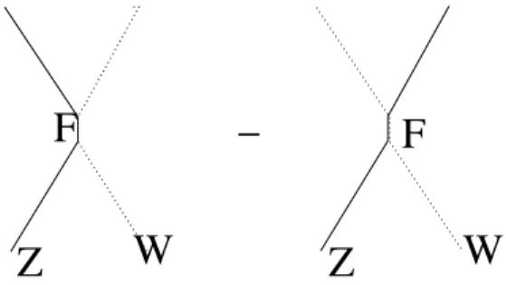
In top pair production, there are three possibilities: if both W ’s decay in leptons then a final state with two high p T leptons, two jets and energy imbalance ( / E T ) from

The 1990’s were marked by the need to extend the theory beyond its usual environments: i) beyond local fields , as strings and branes played a central role in at- tempts at

The short papers in this special issue of the Brazilian Journal of Physics give a broad and deep view on the many topics presented at the workshop and they represent fairly well

The instanton-improved OPE (IOPE) and the analysis of the corresponding Borel sum rules [4] then showed that direct (i.e. small-scale) instan- tons solve two key problems in the

References

[1] D. Berenstein, J. Maldacena, and H. Nastase, arXiv:hep-th/0202021.
[2] G. ’t Hooft, Nucl. Phys. B72, 461 (1974). [3] A. M. Polyakov, arXiv:hep-th/0110196.
[4] J. Maldacena, Adv. Theor. Math. Phys.2, 231 (1998) [Int. J. Theor. Phys.38, 1113 (1998)] [arXiv:hep-th/9711200].
[5] S. S. Gubser, I. R. Klebanov, and A. M. Polyakov, Phys. Lett. B428, 105 (1998) [arXiv:hep-th/9802109].
[6] E. Witten, Adv. Theor. Math. Phys.2, 253 (1998) [arXiv:hep-th/9802150].
[7] O. Aharony, S. S. Gubser, J. Maldacena, H. Ooguri, and Y. Oz, Phys. Rept.323, 183 (2000) [arXiv:hep-th/9905111].
[8] M. Blau, J. Figueroa-O’Farrill, C. Hull, and G. Papadopou-los, JHEP0201, 047 (2001) [arXiv:hep-th/0110242].
[9] R. R. Metsaev, plane wave Ramond-Ramond background,” arXiv:hep-th/0112044.
[10] R. R. Metsaev, A. A. Tseytlin, Phys. Rev. D 63, 046002 (2001) [arXiv:hep-th/0007036]
[11] R. Penrose, Differential geometry and relativity, Reidel, Dor-drecht, 1976, pp. 271-275.
[12] M. Gunaydin and N. Marcus, Class. Quant. Grav. 2, L11 (1985). H. J. Kim, L. J. Romans, and P. van Nieuwenhuizen, Phys. Rev. D32, 389 (1985).
[13] A. Santambrogio and D. Zanon, arXiv:hep-th/0206079.
[14] C. B. Thorn, “Reformulating string theory with the 1/N ex-pansion,” arXiv:hep-th/9405069; R. Giles, L. D. McLerran, and C. B. Thorn, Phys. Rev. D17, 2058 (1978); M. T. Wil-son, L. L. Thorn, L. O. Lindquist, and D. L. Grisham, IEEE Trans. Nucl. Sci.24, 1574 (1977); C. B. Thorn, Phys. Rev. D20, 1934 (1979); C. B. Thorn, Phys. Rev. D 20, 1435 (1979); C. B. Thorn, Phys. Rev. D19, 639 (1979); R. Brower, R. Giles, and C. B. Thorn, Phys. Rev. D 18, 484 (1978); C. B. Thorn, Phys. Rev. D17, 1073 (1978); C. B. Thorn, Phys. Lett. B70, 85 (1977); R. Giles and C. B. Thorn, Phys. Rev. D16, 366 (1977).
[15] L. Motl, arXiv:hep-th/9701025.
[16] R. Dijkgraaf, E. Verlinde, and H. Verlinde, Nucl. Phys. B500, 43 (1997) [arXiv:hep-th/9703030].
Imagem
Figure 1. Diagrams that come from F terms. The two diagrams have a relative minus sign
Referências
Documentos relacionados