The size of prey consumed has been considered an important resource dimension in reptiles and especially in amphibians (Toft, 1985). In general, the size of con-sumers is correlated with the size of their prey (Lima and Magnusson, 1998; Shine et al., 2002; Vitt and Caldwell, 1994), which may have important ecological implications (Roughgarden, 1972). For instance, in Anolis lizards, larger individuals within a population tend to consume larger prey so that overlap among different sized individ-uals may be little (Roughgarden, 1972; Schoener, 1968). Such variation at the individual level is a prevalent phe-nomenon in natural populations (Bolnick et al., 2003)
size when there are too many prey
Araújo, MS.
a*,
Pinheiro, A.
band Reis, SF.
aaDepartamento de Parasitologia, Instituto de Biologia, Universidade Estadual de Campinas – UNICAMP,
CP 6109, CEP 13084-971, Campinas, SP, Brazil
bDepartamento de Estatística, Instituto de Matemática, Estatística e Computação Científica,
Universidade Estadual de Campinas – UNICAMP, CP 6065, CEP 13083-859, Campinas, SP, Brazil
*e-mail: [email protected]
Received September 4, 2006 – Accepted October 30, 2006 – Distributed May 31, 2008 (With 2 figures)
Abstract
Prey size is an important factor in food consumption. In studies of feeding ecology, prey items are usually measured individually using calipers or ocular micrometers. Among amphibians and reptiles, there are species that feed on large numbers of small prey items (e.g. ants, termites). This high intake makes it difficult to estimate prey size consumed by these animals. We addressed this problem by developing and evaluating a procedure for subsampling the stomach contents of such predators in order to estimate prey size. Specifically, we developed a protocol based on a bootstrap procedure to obtain a subsample with a precision error of at the most 5%, with a confidence level of at least 95%. This guideline should reduce the sampling effort and facilitate future studies on the feeding habits of amphibians and reptiles, and also provide a means of obtaining precise estimates of prey size.
Keywords: prey size, estimation, precision, bootstrap, Eupemphix nattereri.
Predadores glutões: como estimar o tamanho das
presas quando o número delas é muito grande
Resumo
O tamanho das presas é uma importante dimensão do nicho trófico. Em estudos de ecologia alimentar, os itens alimen-tares são geralmente medidos individualmente com o uso de paquímetro ou ocular micrométrica. Entre os anfíbios e répteis, há espécies que consomem grande número de itens alimentares pequenos (e.g. formigas, cupins). Esse grande número, por sua vez, torna a estimativa do tamanho das presas consumidas uma tarefa difícil. Desenvolvemos um método para colher subamostras dos conteúdos estomacais desses animais com o objetivo de obter estimativas de tamanho das presas. Especificamente, desenvolvemos um protocolo baseado em uma rotina de bootstrap que permite a obtenção de subamostras com erro de precisão de no máximo 5% e confiança de 95%. Esse método deve diminuir o esforço amostral e facilitar estudos futuros sobre os hábitos alimentares de anfíbios e répteis, além de fornecer um meio de obter estimativas precisas de tamanho de presas.
Palavras-chave: tamanho de presa, estimação, precisão, bootstrap, Eupemphix nattereri.
1. Introduction
work involved, which may increase measurement errors due to fatigue. To apply the latter, it would be helpful to define a subsample size that would yield a precise esti-mate of the size of prey consumed by a given individual while minimizing the measuring effort.
Here, we developed a method based on bootstrap resampling (Davidson and Hinkley, 1997; Efron and Tibshirani, 1993) to evaluate the subsample sizes needed to estimate the sizes of prey found within individual gut contents, with a precision error of at most 5% and a con-fidence of at least 95%. We tested this method on the data of the termite consumer frog Eupemphix nattereri (Leiuperidae).
2. Material and Methods
The specimens of E. nattereri analyzed belonged to the collection of the Museu de Biodiversidade do Cerrado of the Universidade Federal de Uberlândia, and were col-lected in the municipality of Uberlândia (18° 55’ S and 48° 17’ W), in the state of Minas Gerais, southeastern Brazil. A wet/hot summer from October to March and a dry/mild winter from April to September characterize the local climate. The mean annual precipitation is around 1,500 mm, varying from 750 to 2000 mm (Sano and Almeida, 1998). The original vegetation in the region is Brazilian savannah (Cerrado; Oliveira and Marquis, 2002). Frogs were collected in two of the vegetation remnants still present in some areas of the municipal-ity (Goodland and Ferri, 1979). Frogs were killed im-mediately upon collection to avoid degradation of prey items due to digestion, fixed in 10% formalin and later preserved in ethanol 70%.
We analyzed 61 specimens. To develop the sub-sampling procedure, we picked three stomachs among our sample of stomachs: one with a small number of intact prey items (Sample 1; henceforth S1); one with an intermediate number (Sample 2; S2); and one with a large number (Sample 3; S3). In those stomachs, we measured all intact prey items found. In S1 we measured N = 37 termite workers (Termitidae); in S2 we measured 2 soldiers and 134 workers (N = 136; Termitidae); and in S3 we measured N = 507 workers (Termitidae). The total length of each prey item (from anterior tip of the mandi-bles to posterior tip of the abdomen) was measured us-ing an ocular micrometer. Items were stretched out and measured dorsally in order to increase the accuracy of measurements.
We wrote a computer program that draws individual measurements from an empirical sample to build simu-lated subsamples. The program then calculates the mean prey size for each subsample and builds a distribution of those mean prey sizes. With this distribution, one can compute the empirical probability of erring by more than a desired quantity. Below we explain the details of the bootstrap procedure.
For a predefined subsample size k, measures were sampled with replacement from the empirical sample of size N. For example, in S1, for k = 5, five measurements and may generate frequency-dependent interactions
with important ecological and evolutionary implications (Roughgarden, 1972; Taper and Case, 1985).
In terms of the diversity of prey consumed, amphib-ians and reptiles show a continuum that varies from spe-cies with broad niches, which use a wide array of prey taxa (mostly terrestrial arthropods), to those with narrow niches that specialize in one or few taxa, such as ter-mites, ants, ter-mites, and/or Collembola (Caldwell, 1996; Huey et al., 2001; Toft, 1981). At least one such special-ist is always found in dietary studies of communities of amphibians and reptiles (Pianka, 1986; Toft, 1980; Vitt and Caldwell, 1994). For example, species of the genus Physalaemus (Giaretta and Menin, 2004; Ryan, 1985; Vitt and Caldwell, 1994) and many species in the families Bufonidae and Microhylidae (Caldwell and Vitt, 1999) are known to be specialists in termites and ants; many lizard species are also know to specialize in these type of prey (Huey et al., 2001; Pianka, 1986; Schoener, 1968); finally some snakes are also specialized in ants (e.g. Ramphotyphlops nigrescens; Shine and Webb, 1990), or both ants and termites (e.g. Leptotyphlops koppesi; R. J. Sawaya, unpubl. data).
Most studies dealing with food habits rely on gut-content analysis to obtain information on prey sizes and taxa (Caldwell, 1996; Roughgarden, 1974; Schoener, 1968; Vitt and Caldwell, 1994). When dealing with those specialist predators, one can find very large num-bers of prey items in a given stomach. For instance, in an analysis of the stomach contents of the ant-specialist poison frog Dendrobates auratus the number of prey items per stomach varied from 15 to 453 (Caldwell, 1996). In Physalaemus fuscomaculatus, this number varied from 1 to 256 (Giaretta and Menin, 2004), and the mean number of termites per stomach in large Bufo marinus was 105.8 (Strüssmann et al., 1984). Finally, in the blindsnake Ramphotyphlops nigrescens, which feeds mainly on ant pupae and larvae, the number of prey items per individual varied from 1 to 1,431 (Shine and Webb, 1990).
ing by more than 5% around the sample mean. For exam-ple, in S1, in order to be considered precise, a subsample mean must fall between the limits 5.22, and 5.48 mm (Figure 1a). Looking at the y-axis, we can determine those precision limits, and the tails of the different curves that are out of these limits. These tails represent the sub-samples whose means fell out of the precision limits. By looking at the x-axis, in turn, we can determine the percentiles associated with these tails. For example, for were sampled with replacement from the 37
measure-ments of S1 to build one subsample. Ten thousand such subsamples were bootstrapped from S1, and the mean prey size of each subsample was calculated. A distribu-tion of these mean values was then built, and the process was repeated for a different k value. Different k-values were arbitrarily defined based on the size of each sam-ple. For example, in S1, subsamples were k = 5, 10, 19. This whole process was done for S1, S2, and S3, for each subsample size k. The procedure is outlined in the fol-lowing algorithm:
Let N = sample size (1)
Let x1,x2,..,xN be the recorded values (2)
Let k N
2 , N
5 , N 10 ,
N 20 ,
N 50 ,
N
100 (3)
For b = 1 to 10,000, choose x1 , ,bxkb from
x1, ,xN with replacement (4)
x
k x
kb ib i
k 1
1 (5)
qk( )α α th quantile from x1, ,x10 000, (6)
Choose the smallest k such that qk(1 α) qkα 2ε , for a precision error of ε and confidence of 100
(1-2α)% (7)
We defined a precision error εof 2.5%, so that a sub-sample was considered precise if its mean fell within the interval of the empirical mean ±ε. This gives us a pre-cision of 5% around the empirical mean (“true” mean). We defined α as 2.5%, so that a subsample size k was considered acceptable if only a maximum of 2.5% of subsample means were larger than the upper limit of precision, and at most 2.5% of them were smaller than the lower limit of precision. This gives us a subsample size k whose means will fall within the precision limits with a 95% probability. This way, for each sample Si, we can define the smallest subsample size k that will yield a mean value with an error of at most 5%, with a prob-ability of at least 95%. The code was written in Matlab, and is available from the authors upon request.
3. Results
The sample mean prey sizes ±ε were: 5.35 ± 0.13 mm (S1; Figure 1a); 7.87 ± 0.20 mm (S2; Figure 1b); and 4.40 ± 0.11 mm (S3; Figure 1c). In S1, subsample sizes were k = (5, 10, 19; Figure 1a); in S2 they were k = (5, 10, 25, 50, 100; Figure 1b); and in S3 they were k = (5, 10, 25, 50, 100, 250; Figure 1c). For each subsample size, the subsample means were computed and the quantiles of these values were recorded. Using these quantiles, we were able to compute the empirical probabilities of
err-k = 5 k = 10 k = 25 k = 50 k = 100
Mean pre
y size (mm)
Percentiles 7.0
8.8 8.6 8.4 8.2 8.0 7.8 7.6 7.4 7.2
0 10 20 30 40 50 60 70 80 90 100
4.0 4.1 4.2 4.3 4.4 4.5 4.6 4.7 4.8
Mean pre
y size (mm)
Percentiles
0 10 20 30 40 50 60 70 80 90 100 k = 5 k = 10 k = 25 k = 50 k = 100 k = 250 k = 5 k = 10 k = 19
Percentiles
Mean pre
y size (mm)
0 10 20 30 40 50 60 70 80 90 100 5.4
5.2 5.0 5.6 5.8
6.0 a
b
c
Figure 1. Bootstrap error for different subsample sizes.
items in a given individual (e.g. Shine and Webb, 1990). Although having the advantage of simplicity, this method only provides information on the range of the data and ignores the distribution of resources used by individuals. Another possible method would be to measure only one or a few individuals of similar sized prey and assign the same size to the remaining prey. Our results demonstrate, however, that this method is inadequate because it may yield estimates that largely depart from the ‘true’ empiri-cal mean. Finally, the alternative of measuring all prey items in a given stomach, besides being time consum-ing, may actually increase errors during measurement because of fatigue of the researcher. As a consequence, it would be useful to have a subsampling procedure in order to deal with such cases.
The precision of a subsample estimate depends on the relative (henceforth kR) and absolute (henceforth kA) sizes of the subsample (relative and absolute precisions, respectively; Hansen et al., 1993). Subsampling theory predicts that the relative precision decreases with de-creasing relative size (Hansen et al., 1993). In fact, this can be clearly seen in our results as, for instance, in S3 a subsample of kR = 10% was satisfactory according to our criteria, whereas kR = 5% was not (Figure 1c). Likewise, according to the central limit theorem (Feller, 1968), a reduction in the absolute size of subsamples decreases the precision of the estimate of the parametric mean (µ), rendering impossible to obtain precise estimates below a certain absolute value (Hansen et al., 1993). Therefore, both the relative and absolute sizes of the subsamples must be considered when developing a protocol to esti-mate prey size.
Ideally, we would like to use the smallest subsample possible to reduce measurement effort. As a first step, we can for the three analyzed samples, choose the smallest acceptable kR in each sample, and among those pick the smallest, which is kR = 10% in S3. Although kR = 10% worked fine in S3, it would not yield precise estimates in either S1 or S2. The explanation for this relies on the absolute precision because, as stated before, it is not possible to obtain a precise estimate below a certain ab-solute value. For example, in S2 (N = 136), kR = 10% corresponds to a kA = 14 items. As a result, we cannot simply define kR = 10% as the optimal subsample size, because for samples smaller than N = 500, in which 10% of prey items will be less then 50 items, kR = 10% is not warranted. To circumvent this problem, we can define the subsample size in terms of its absolute size kA; in S3, kR = 10% corresponds to kA = 50. We now fix our atten-tion on kA and check if it works in the other samples. As we have seen, kA = 50 is satisfactory in S2; in the case of S1, it would oblige us to measure all 37 items, which would yield the best estimate possible. Regarding rela-tive precision, kA = 50 will always yield kR> 10% for N < 500, so that the relative precision will not be com-promised. On the other hand, there is no guarantee that for N > 500 (e.g. N = 700) kA = 50 would yield a precise estimate. This is because in a sample of N = 700, kA = 50 k = 5 in S1 (the outermost curve), around 30% of
subsam-ples had means smaller than 5.22 mm, and around 30% (100-70%) had means larger than 5.48 mm (Figure 1a). So, by taking a subsample of k = 5 in S1, one would es-timate an imprecise mean with a probability of about 60%. Now, instead of fixing our attention on a specific k-curve, we can look at all the curves and check the cor-responding percentile values at which they are crossed by the precision limits. For example, in S1 for the larger subsample size (k = 19) around 15% of the subsamples had means smaller than 5.22 mm, and 15% (100-85%) had means larger than 5.48 mm, so that one would err with a probability of 30% by measuring 19 items. In the case of S1, therefore, all prey items should be measured, which would yield the best estimate possible for that sample. By doing the same procedure in S2, we can see that for k = 50, around 2.5% of the subsample means fell out of the lower precision limit, and around 2.5% out of the upper limit, indicating that precise estimates will be obtained with a probability of 95% for this k-value (Figure 1b). In the case of S3, it is possible to have pre-cise estimates with a probability of 95% with k = 50 (Figure 1c). Therefore, according to our results, in S1 we should measure all items; in S2 we should measure 50 items (37% of the sample); and in S3 we should meas-ure 50 items (10% of the sample).
4. Discussion
We have demonstrated numerically that the precision of the estimates of prey size in gut contents is sensitive to the size of the subsamples, which is in accordance with the analytical predictions of subsampling theory (Hansen et al., 1993). Below, we 1) discuss the implications of these results for the estimation of prey size in consum-ers in which a large number of prey items is found in individual gut contents, 2) develop a protocol that can be used in other studies, and 3) discuss the further use of the protocol in future studies.
When investigating patterns of resource use of ani-mals, researchers are often interested in within-popu-lation differences, such as those between sexes or age classes (Lima and Magnusson, 1998; Shine et al., 2002) and between individuals (Bolnick et al., 2003; Smith and Skúlason, 1996). In principle, if there is a large variation between the groups being compared (e.g. males versus females), even fairly large within-group errors may have little effect on the detection of existing differences (Rao, 1973). However, in cases where between-group differ-ences are subtle, the lack of precision of estimates may cause type II errors (Rao, 1973), in which researchers will believe groups are equal when they are not. In fact, ecologists will never know a priori the amount of varia-tion among the individuals sampled, so that the precision of estimates may be a prerequisite for the very quantifi-cation of this variation.
tors (Pianka, 1986; Toft, 1980). The procedure described here should provide a guideline for authors to obtain pre-cise estimates of prey size when dealing with amphib-ians and reptiles that feed on large numbers of prey at a given meal. Moreover, it should reduce the sampling effort and consequently facilitate future studies dealing with prey size estimation.
Acknowledgements –– We thank A. Giaretta for permission to use the specimens in the collection of the Museu de Biodiversidade do Cerrado of the Universidade Federal de Uberlândia. G. Machado and R. Constantino helped in identifying the termites. P. Guimarães Jr. made useful suggestions on the manuscript, and S. Hyslop reviewed the English. Financial support was provided by FAPESP. MSA and SFR were supported by fellowships from CAPES and CNPq, respectively. AP thanks FAPESP and CAPES for financial support.
References
ADAMS, DC. and ROHLF, FJ., 2000. Ecological character displacement in Plethodon: biomechanical differences found from a geometric morphometric study. Proc. Natl. Acad. Sci. U. S. A., vol. 97, no. 8, p. 4106-4111.
BOLNICK, DI., SVANBÄCK, R., FORDYCE, JA., YANG, LH., DAVIS, JM., HULSEY, CD. and FORISTER, ML., 2003. The ecology of individuals: incidence and implications of individual specialization. Am. Nat., vol. 161, no. 1, p. 1-28.
CALDWELL, JP., 1996. The evolution of myrmecophagy and its correlates in poison frogs (Family Dendrobatidae). J. Zool., vol. 240, no. 1, p. 75-101.
CALDWELL, JP., and VITT, LJ., 1999. Dietary asymmetry in leaf litter frogs and lizards in a transitional northern Amazonian rain forest. Oikos, vol. 84, no. 3, p. 383-397.
DAVIDSON, AC., and HINKLEY, DV., 1997. Bootstrap methods and their application. Cambridge: Cambridge University Press.
DIMMITT, MA., and RUIBAL, R., 1980. Exploitation of food resources by spadefoot toads (Scaphiopus). Copeia, vol. 1980, no. 4, p. 854-862.
EFRON, B., and TIBSHIRANI, RJ., 1993. An introduction to the bootstrap. Boca Raton: Chapman and Hall/CRC, p. 436. FELLER, W., 1968. An introduction to probability theory and its applications. New York: John Wiley and Sons, p. 704. GIARETTA, AA., ARAÚJO, MS., MEDEIROS, HF., and FACURE, KG., 1998. Food habits and ontogenetic diet shifts of the litter dwelling frog. Proceratophrys boiei (Wied). Rev. Bras. Zool., vol. 15, no. 3, p. 385-388.
GIARETTA, AA., and MENIN, M., 2004. Reproduction, phenology and mortality sources of a species of Physalaemus (Anura: Leptodactylidae). J. Nat. Hist., vol. 38, no. 13, p. 1711-1722.
GOODLAND, R., and FERRI, GM., 1979. Ecologia do Cerrado. Belo Horizonte: Livraria Itatiaia.
HANSEN, MH., HURWITZ, WN., and MADOW, G., 1993. Sample survey methods and theory. New York: John Wiley and Sons.
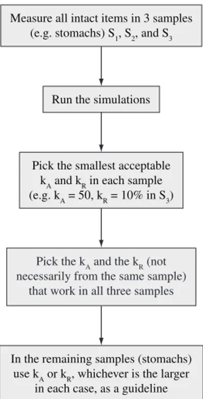
corresponds to a subsample of relative size less than 10%, and the relative precision may be compromised. The solution for the cases with N > 500 is to prioritize kR instead of kA. So, for example, in the hypothetical case of N = 700 the appropriate subsample would be kR = 10% (kA = 70). Therefore, for N < 500, subsamples should be kA = 50, and for N > 500 they should be kR = 10%. As a conclusion, in our data set in general the rule to be applied is kR = 10% or kA = 50 items, whichever is the larger. As a general rule, one should pick the small-est acceptable kA and kR values and choose among them the one kA and kR values that work for all three samples. Figure 2 illustrates the steps involved in our protocol.
In studies dealing with amphibians and reptiles spe-cialized in small-sized prey (e.g. termites, ant, mites, Collembola), it is likely that a large proportion of speci-mens will have large numbers of prey items in their stom-achs (e.g. Dimmitt and Ruibal, 1980). Moreover, many species (e.g. lizards; Pianka, 1986; Schoener, 1986) feed on termite swarms, which represent an unpredict-able and temporarily abundant food resource that may be consumed in large amounts by individuals. Moreover, since termites and ants are relatively small-sized prey and their nests have a patchy distribution, they are gener-ally consumed in large numbers when found by
preda-Measure all intact items in 3 samples
(e.g. stomachs) S1, S2, and S3
Run the simulations
Pick the smallest acceptable
kA and kR in each sample
(e.g. kA = 50, kR = 10% in S3)
Pick the kA and the kR (not necessarily from the same sample)
that work in all three samples
In the remaining samples (stomachs)
use kA or kR, whichever is the larger
in each case, as a guideline
SHINE, R., REED, RN., SHETTY, S. and COGGER, HG., 2002. Relationships between sexual dimorphism and niche partitioning within a clade of sea-snakes (Laticaudinae). Oecologia, vol. 133, no. 1, p. 45-53.
SHINE, R., and WEBB, JK., 1990. Natural history of Australian typhlopid snakes. J. Herpetol., vol. 24, no. 4, p. 357-363. SMITH, TB., and SKÚLASON, S., 1996. Evolutionary significance of resource polymorphisms in fishes, amphibians, and birds. Annu. Rev. Ecol. Evol. Syst., vol. 27, p. 111-113. STRÜSSMANN, C., VALE, MBR., MENEGHINI, MH., and MAGNUSSON, WE., 1984, Diet and foraging mode of Bufo marinus and Lepdactylus ocellatus. J. Herpetol., vol. 18, no. 2, p. 138-146.
TAPER, ML., and CASE, TJ., 1985. Quantitative genetic models for the coevolution of character displacement. Ecology, vol. 66, no. 2, p. 355-371.
TOFT, CA., 1985. Resource partitioning in amphibians and reptiles. Copeia, vol. 1985, no. 1, p. 1-21.
-, 1981. Feeding ecology of Panamanian litter anurans: patterns in diet and foraging mode. J. Herpetol., vol. 15, no. 2, p. 139-144.
TOFT, CA., 1980. Feeding ecology of thirteen syntopic species of anurans in a seasonal tropical environment. Oecologia, vol. 45, no. 1, p. 131-141.
VITT, LJ., and CALDWELL, JP., 1994. Resource utilization and guild structure of small vertebrates in the Amazon forest leaf litter. J. Zool., vol. 234,no. 4,p. 463-476.
HUEY, RB., PIANKA, ER., and VITT, LJ., 2001. How often do lizards “run on empty”? Ecology, vol. 82, no. 1, p. 1-7. LIMA, AP., and MAGNUSSON, WE., 1998. Partitioning seasonal time: interactions among size, foraging activity and diet in leaf-litter frogs. Oecologia, vol. 116, no. 2, p. 259-266. OLIVEIRA, PS., and MARQUIS, RJ., 2002. The cerrados of Brazil: ecology and natural history of a neotropical savanna. New York: Columbia University Press, p. 424.
PIANKA, ER., 1986. The ecology and natural history of desert lizards. Analyses of the ecological niche and community structure. Princeton: Princeton University Press.
RAO, CR., 1973. Linear statistical inference and its applications. New York: John Wiley and Sons.
ROUGHGARDEN, J., 1972. Evolution of niche width. Am. Nat., vol. 106, no. 952, p. 683-718.
-, 1974. Niche width: biogeographic patterns among Anolis lizard populations. Am. Nat., vol. 108, no. 962, p. 429-442. RYAN, MJ., 1985. The Túngara Frog: A Study in Sexual Selection and Communication. Chicago: The University of Chicago Press, p. 246.
SANO, SN., and ALMEIDA, SP., 1998. Cerrado: Ambiente e Flora. Planaltina, GO: Embrapa-CPAC, p. 556.
SCHOENER, TW., 1968. The Anolis lizards of Bimini: resource partitioning in a complex fauna. Ecology, vol. 49, no. 4, p. 704-726.