A Work Project, presented as part of the requirements for the Award of a Masters Degree in Finance from the NOVA – School of Business and Economics
MOMENTUM RISK: AN APPROACH FOLLOWING THE
CORRELATIONS BETWEEN ACTIVE STOCKS
DAVID BORGES PINHEIRO – 635
A Project carried out on the Finance course, under the supervision of: Professor Pedro Santa-Clara
MOMENTUM RISK: AN APPROACH FOLLOWING THE
CORRELATIONS BETWEEN ACTIVE STOCKS
Abstract
The momentum anomaly has been widely documented in the literature. However, there are still many issues where there is no consensus and puzzles left unexplained. One is that strategies based on momentum present a level of risk that is inconsistent with the diversification that it offers. Moreover, recent studies indicate that this risk is variable over time and mostly strategy-specific. This work project hypothesises and proves that this evidence is explained by the portfolio constitution of the momentum strategy over time, namely the covariance and correlation between companies in the top and down deciles and across them.
1. General Overview:
1.1: Introduction:
The Momentum anomaly has been recurring in asset returns. Strategies based on the idea that recent winners outperform recent losers have provided high returns. But they have come alongside with inconsistent levels of risk.
The evidence on momentum was found for the first time by Levy (1967). In his findings, the best group had 9.6% 6-month average return while the worse only averaged 2.9%. But it was only Jegadeesh and Titman (1993) who properly scrutinized it, finding a 12.01% average annual return for their prime portfolio of winners minus losers. Over the last two decades momentum has been the focus of numerous studies and has been discovered in different asset classes (Antonacci (2013)) and geographic regions (Griffin, Ji and Martin (2003)).
However, the big subject around momentum is the economic puzzles that it encompasses. The first concerns its abnormal returns, represented by its large alpha. This means that, as pointed out in Fama and French (1996), momentum excess returns cannot be explained by its relation with the market excess return or even by a multifactor model such as the Fama-French three-factors model. Studies about this puzzle, such as Jegadeesh and Titman (2001), have been repeatedly documented, debating possible explanations that cover data mining, behavioural biases and compensation for risk.
that it brings (Barroso and Santa-Clara (2012)). Finally, the risk has a time-varying effect and is very predictable, as studied by Daniel and Moskowitz (2012).
1.2: Literature review:
As pointed in the previous sub-section, momentum risk features the most interesting and less covered puzzle. The first relevant study about this subject is that of Grundy and Martin (2001). They identified market risk to be the main source of momentum risk and its predictability, since momentum had negative betas after bear markets and positive betas after bull markets. One decade later, Daniel and Moskowitz (2012) contested the previous model of linear betas and developed a new one based on the high-frequency beta of daily returns. Nevertheless, the direction of their thoughts and findings was the same.
More recently, Barroso (2013) added to the defence of market-driven risk as the source of momentum risk behaviour his bottom-up beta of momentum. He found that this weighted average beta of individual betas of stocks in the portfolio explained 39.59% of momentum risk. He also found that a high beta with respect to the market forecasts both lower returns and higher risk in the future, with a stronger effect on the second.
However, none of these authors were able to avoid momentum crashes. This leads to the possibility that only by hedging the other component of risk, the specific risk1, might be possible to hedge against downward situations.
The study of this specific component of momentum is well covered in Kang and Li (2007), where it is considered the third source of return predictability and the biggest
1 Specific risk here is not the result of low diversification in the portfolio but a consequence of
part of momentum profits. Nevertheless, the application of strategy-specific risk to explain momentum risk was only definitely proposed by Santa-Clara and Barroso (2012). They attributed to this component the major influence on their three major findings on momentum risk: high magnitude (too much risk despite the high Sharpe ratio: 15.03% average volatility for momentum compared to 12.81% for the market); variation over time (time-varying effect supported by a 12.26% standard deviation of realized volatility against only 7.82% for the market portfolio); and persistency.
1.3. Purpose of the Project:
This project will embark on the study of momentum, following the more recent and less covered findings and presenting previously unseen results. Therefore, the bottom line is the momentum risk puzzle and the course of action regards its specific component. To start, the most interesting findings in Barroso and Santa-Clara (2012) will be confirmed and replicated, namely those regarding the magnitude and time-variation of momentum risk, as well as the influence of strategy-specific risk in these. Then, these findings will be explained following the hypothesis that the drivers of specific risk are the correlations between the stocks of companies present in the long and short deciles. Correlations that will be assessed for stock residuals instead of returns because only the specific component is under analysis.
2. Discussion:
2.1 Data:
This work project uses the same monthly data as in Barroso (2013), taken from the Centre for Research in Security Prices (CRSP) and corresponding to all listed stocks in the NYSE, AMEX or NASDAQ from January 1950 until December 2010. In total, 22.998 companies were considered in the sample. Individual monthly data for each security was taken regarding stock prices and gross dividend returns.
Furthermore, monthly data for the Fama-French Three-Factor Model (market risk premium (RMRF), small minus big factor (SMB) and high minus low factor (HML)) were taken from Kenneth French’s data library, comprising monthly data from January 1950 to December 2010.
2.2. The Momentum Strategy and its Risk:
The strategy used to capture the momentum effect follows a relative strength methodology that selects stocks based on their returns over a certain number of months and holds them for another pre-determined period.
Following the same approach in Daniel and Moskowitz (2012) and Barroso and Santa-Clara (2012), in every month t, cumulative returns1 from t-12 to t-2 were used to rank stocks2 into ten groups3. The momentum portfolio was constructed by buying the best performing group and selling short the worse performing one. These positions were maintained during the 1-month holding period considered. As most literature suggests, it was kept a 1-month gap between the end of the ranking period (t-12 to t-2) and the beginning of the holding period (t), in order to avoid spurious results from the
2 Only stocks with valid returns from t-12 to t-2 and at t were considered.
term reversal effect usually observed in stock returns. Finally, regarding the weighting of stocks in the active deciles, equal weights were preferred over value weights, to avoid an erroneous size effect in the results.
Momentum produces superior cumulative returns when compared to the portfolios built based on each Fama-French factor, as depicted in Figure 1. An investor who had chosen the momentum strategy in early 1956 would achieve a total 519.81% cumulative return after 60 years, while a similar investment on the market portfolio would only give a cumulative result of 404.16%. Moreover, Table 1 indicates that the momentum average return of 9.70% is above the 7.05% for the market risk factor. The Sharpe ratio, however, is slightly below of that of the market, but one needs to remember that momentum offers this for a zero investment endowment. These results are in line with the aforementioned literature supporting momentum, and differ from the 12.30% average annual return found in the Kenneth French Data Library for the same period of time due to the data selection process.
Regarding risk, momentum presents a volatility level that is much higher than that of the market portfolio (21.68% against 15.03%, respectively). Furthermore, the high excess kurtosis (20.34) and the pronounced negative skew (-2.35) indicate that returns are far from normal. These results support the existence of a magnitude issue in momentum, as pointed out by Barroso and Santa-Clara (2012), and are very close to the 20.38% average yearly volatility found in the Kenneth French Data Library for the period analysed.
𝑅𝑉𝑖𝑡 =
∑𝑡−60𝑡−2 𝑟𝑖𝑡2
60 (1)
where i stands for each factor and t for each point in time.
Figure 2 shows that there are three interesting periods in terms of volatility: 1975, 2000 and 2008. In all, the realized volatility of momentum experience spikes, which coincide with periods in which the cumulative returns increase, suffer considerable changes and decrease afterwards. For the periods around years 2000 and 2008 the market premium factor also undergo similar (but in lower magnitude) volatility behaviour, thus explaining some of the variation, as the dot-com bubble and the 2008 crisis coincide with these dates, respectively. For the period of 1975, it seams that the source of extra volatility is solely specific to momentum.
For the full sample, momentum volatility is stronger and varies more over time than that of the Fama-French factors. Regarding the first finding, the mean realized volatility is 18.91% for momentum, compared to the 14.67% for the market premium. In what concerns the second, the volatility of risk is 8.58% for the WML portfolio while the RMRF portfolio’s standard deviation of risk was only 2.71% during the period considered. These results go in line with Barroso and Santa-Clara (2012), despite the differences in magnitude coming from the historic period considered.
2.3. Risk Analysis:
2.3.1. Decomposition of Momentum Risk: Market vs. Specific Components:
As aforementioned, total returns from momentum include both a market component (RMRF) and a specific component:
𝑟𝑚𝑜𝑚𝑡 = 𝛼 + 𝛽𝑡−1𝑟𝑟𝑚𝑟𝑓𝑡+ 𝜀𝑚𝑜𝑚𝐶𝐴𝑃𝑀𝑡 (2)
When the analysis is done at an individual level as in this paper, the decomposition can be expressed in the following way:
∑ 𝑤𝑖𝑡𝑟𝑖𝑡 = ∑ 𝑤𝑖𝑡𝛽𝑖𝑡𝑟𝑟𝑚𝑟𝑓𝑡+ ∑ 𝑤𝑖𝑡𝜀𝑖𝐶𝐴𝑃𝑀𝑡 (3)
where i stands for each company in the portfolio.
Thus, regarding risk, a similar decomposition can be performed:
𝜎𝑚𝑜𝑚2 𝑡 = 𝛽𝑡2𝜎𝑟𝑚𝑟𝑓2 𝑡+ 𝜎𝜀2𝑡 (4)
The market component equals the squared standardized linear beta from a regression of momentum returns on the market excess return4 times the variance of the RMRF factor. The individual component is then obtained from the difference between total and market-driven risk.
The results in Table 2 go in line with Barroso and Santa-Clara (2012). The market risk component only covers a small part of momentum total risk (5.77%, on average), leaving to the specific component the major part of its magnitude (94,23%, on average). Furthermore, the average annual specific risk is 18.44%, very close to the total risk, while the market component is only on average 3.17%, annualized. Regarding the variability over time, the volatility is also very similar for total and specific risk (8.58% and 8.56%, respectively, compared to the 2.76% of market-driven volatility). The small
4 Other more advanced models such as the Bottom-Up approach of Barroso (2013) were
influence of market risk is consistent over time, with the specific component following a similar behaviour as total risk, with spikes in the same periods.
Thus, the results confirm the hypothesis that specific risk corresponds to the major component of momentum risk both in magnitude and time variation. So, it deserves an even deeper evaluation, to extract what drives this source of risk.
2.3.2. Decomposition of Specific Risk: Variance vs. Covariance Components:
In order to properly study the strategy-specific risk, it was decomposed into its two components: variance of each stock and covariance between every two stocks. To better understand the covariance component and its real source, this part is further split into three: covariance among winners, covariance among losers and covariance between stocks in separate deciles, in the following way:
𝜎2(∑ 𝑤
𝑖𝑡𝜀𝑖𝑡) = ∑ 𝑤𝑖 2𝑖𝜎2(𝜀𝑖) + 2 ∑ 𝑤𝑖≠𝑗 𝑖𝑤𝑗𝐶𝑜𝑣(𝜀𝑖𝑊𝑊, 𝜀𝑗𝑊𝑊) + 2 ∑ 𝑤𝑖≠𝑗 𝑖𝑤𝑗𝐶𝑜𝑣(𝜀𝑖𝐿𝐿, 𝜀𝑗𝐿𝐿) −
−2 ∑ 𝑤𝑖≠𝑗 𝑖𝑤𝑗𝐶𝑜𝑣(𝜀𝑖𝑊𝑊, 𝜀𝑗𝐿𝐿) (5)
where i and j stand for different companies in the portfolio; WW is used when the company is in the winner’s decile and LL when it is in the loser’s decile.
Each component was calculated having in mind that individual stocks have equal weights on the momentum portfolio. For stocks in which the strategy is long a positive weight was assigned while those in the short side took negative positions.
overstate these correlations. So, the residuals for each company at every point in time are obtained from a regression of individual gross dividend returns5 on the market risk-premium.
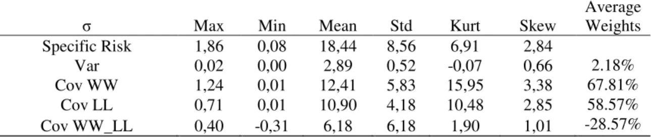
Table 3 resumes the most important statistics of the decomposition of specific risk. As observable, the covariance part is the most significant. Together, covariances account for 97.82% of momentum specific risk against only 2.18% of variances. This confirms what is expected from the formula, meaning that the high specific risk comes from the interaction between stocks.
However, more important is to understand which covariance drives more of the specific risk. The weights of 67.81% for winner’s intra covariance component and 58.57% for loser’s intra covariance component are the most significant. The inter covariance has a
negative weight of 28.57% because of the positions (one negative – loser –, and one positive – winner). The average value of the covariance over time is also higher for the intra covariance (12.41% and 10.90%, respectively for winners and losers) than for the cross covariance (6.18%). However, despite that intra deciles covariance are behaving as expected, the inter group covariance is actually contributing to a decrease in total specific risk, contrarily to the initial hypothesis. Thus, it is safe to conclude that it is the average covariance present among winners and among losers that contribute to such high strategy-specific risk and thus an abnormally high momentum risk. Nevertheless, the higher contribution of the winner’s side compared to the loser’s side is not
significant to consider that the former has consistently a higher influence.
Regarding the time-varying risk of momentum, the standard deviations of each component of specific risk indicate that the covariance part is the main responsible for
it. While the variance component has an annual standard deviation over time of 0.52%, the covariance components have standard deviations of 5.83%, 4.18% and 6.18%, respectively for winners, losers and between them. Thus, there evidence that the covariance is also the most important component of time-varying risk, despite that there is not a group that significantly contributes more for the full sample.
Having a look at Figure 3, the periods of 1975, 2000 and 2008 are relevant again. In the first, the volatility of the winner’s covariance component contributes most to the
volatility peak. In 2000 and 2008 both the winners and the cross covariance components contribute to this period of highest volatility. Overall, it is clear that the covariance among winners and between groups are the ones that varies more side by side with total risk, especially in the critical periods. The other covariance component seams to vary more randomly and thus contribute much less in terms of time-variation of risk.
The results in this sub-section prove that the driver of specific risk, both in magnitude and variation is the covariance part, in line with the thesis proposed for this work project. However, despite that the long side shows signs of bigger influence, there is no conclusive evidence on which side is stronger.
2.3.3. Analysis of Covariance through Correlation:
Since covariance is the most important component of momentum specific risk, it is important to add to the analysis what drives this covariance. By definition, the covariance and correlation between two stocks i and j are intrinsically connected:
𝐶𝑜𝑣(𝑖, 𝑗) = 𝜎𝑖𝜎𝑗𝐶𝑜𝑟𝑟(𝑖, 𝑗) (6)
momentum strategy, each residual’s covariance was studied through its corresponding correlation component regarding two further issues. The first was to compare the residuals obtained from the CAPM with a series of residuals obtained by the same process but using the Fama-French 3-Factor Model (FF). The usage of this latter model allows removing the size and book-to-market effects from the specific component of returns. The second was to calculate also ex post correlations, based on the 12 monthly residuals after the holding period. The difference between the ex ante and ex post correlations allows understanding whether correlations already existed or if they only appear or become stronger after being included in the strategy.
Regarding the comparison between CAPM residuals and Fama-French residuals, Table 4 compacts the statistical information regarding the six series of correlations for winners, losers and between them, for both models. The results presented go in line with the hypothesis made. Regarding the CAPM residuals, the average past correlation is clearly positive for the winner’s and loser’s deciles (10.37% and 9.81%, respectively)
while for the cross deciles correlation is close to zero. In what concerns the FF residuals, correlations are, in general, lower. The negative average past cross correlation of -3.49% indicate that this component is forcing the risk to increase, in line with the intra group correlations.
economically significant. Thus, this should be an issue to consider in the analysis of momentum risk.
The evidence that CAPM and Fama-French residuals behave similarly show that the inclusion of a size and market-to-book components does not change the behaviour of the specific component of companies’ returns in the momentum strategy. Nevertheless,
the fact that the first are significantly higher that the second may indicate that part of the magnitude, of momentum residual correlations can be explained by one or both of these factors, but a part remain present from another possible source.
Figure 4 allows evaluating the long-run evidence on average correlations. Despite that there is no clear path on correlations over time, the winners decile for CAPM have two volatility spikes around 1975 and 2000. While in 1975 it is accompanied by positive cross correlations, in 2000, it is sided with a negative spike of cross correlations. The FF residuals suffer much less fluctuations, with only slight spikes, such as 1982 for loser’s decile and 2000 for winner’s decile. These results indicate that while in 1975 the peak
seem to come from the size or book-to-market factors; in 2000, corresponding to the dot-com bubble, the similarity in the behaviour of both residuals indicate that is the market factor that is driving these correlations. These observations are consistent with the spikes of total momentum volatility and so denote an important explanation for its occurrence.
From a time-varying point of view, Table 4 shows that for CAPM residuals the correlations among winners have a stronger standard deviation (4.57%, monthly) than the other two groups (bellow 3%, monthly). However, the FF residuals’ correlations do
suffered turbulent periods around 1975, 2000 and 2008, especially for the CAPM residuals but also for the Fama-French series, in line with what was found for total momentum risk, so proving that the volatility in correlations are driving momentum risk in crash periods.
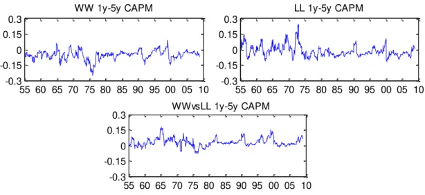
In what concerns the comparison between ex ante and ex post correlations, Table 5 represent the descriptive statistics for the differences between the two. Contrarily to the behavioural view, there is no clear path indicating that companies become more correlated once they are added to the strategy. If something, it is the opposite case, with average differences (1 year minus 5 years) being negative among deciles (-5.20 percentage points and -1.46 percentage points for winners and losers, respectively, with residuals from CAPM). It is only the cross correlation that increases, by 3.09 percentage points, on average, which also goes against the behavioural approach. These findings, which are significant at 5% confidence level, mean that when companies are included in the same decile the correlations among them decrease, on average, while their correlations increase when they are selected to opposite deciles. Thus, correlations were already present with the expected signals before the holding period, and move to the opposite direction when included in the strategy.
The number of positive correlations confirms the aforementioned results in magnitude (10.03% and 29.48% for the in decile correlations and 84.10%% for the cross decile correlations).
3. Conclusion:
This work project studied and revealed new interesting results regarding the momentum risk puzzle that compose a significant advance for its understanding.
Using a very large sample, it is confirmed that momentum risk is too high (21.68% annual average) and variable over time (8.58% annual change in standard deviation). Moreover, it is verified that the specific component of the strategy’s risk is by far the main responsible for these two findings, accounting for almost 95% of it, on average. The existing relations between total and specific-risk provided evidence that the main driver of momentum risk is the covariance that exists between the companies that are included in the strategy, explaining almost 98% of its magnitude, on average. This covariance comes from the individual characteristics of these stocks rather than from the common market component. Moreover, it is the volatility of the covariance component over time that explains most of the time-varying behaviour of momentum total risk. Nonetheless, while it is clear that the high risk comes from the covariance between residuals of stocks that are in the same decile (either winners or losers); the source of the time-varying effect is not so obvious, with the covariance among winners and between deciles taking the lead.
The sub period analysis allowed extracting three periods that are critical in terms of momentum risk for its magnitude and volatility: 1975, 2000 and 2008. The existence of spikes during these three periods for covariances and correlations, with a stronger effect of the long side, supports the conclusion that they these components are crucial during the crash periods in the sample examined.
findings discard a behavioural explanation and indicate that the relation present may come from the individual characteristics that already existed. Moreover, part of the risk magnitude comes from a size and book-to-market effects, as drawn from the comparison of results using CAPM and Fama-French based residuals.
4. References:
Antonacci, Gary. 2013. “Risk Premia Harvesting Through Dual Momentum”. Working
Paper.
Barroso, Pedro. 2013. “The Bottom-Up Beta of Momentum”. Working Paper.
Barroso, Pedro & Santa-Clara, Pedro. 2012. “Momentum has its moments”. Working Paper.
Daniel, Kent & Moskowitz, Tobias. 2012. “Momentum Crashes”. Swiss Finance
Institute Research Paper No. 13-61.
Fama, Eugene F. & French, Kenneth R. 1996. “Multifactor Explanations of Asset Pricing Anomalies”, The Journal of Finance, vol. 51, no. 1: 55-84.
Griffin, John M., Ji, Xiuqing & Martin, J. Spencer. 2003. “Global Momentum Strategies: A Portfolio Perspective”. Working Paper.
Grundy, B., & Martin, J. S. 2001. “Understanding the nature of the risks and the source of the rewards to momentum investing”. The Review of Financial Studies, 14: 29-78.
Jegadeesh, Narasimhan & Titman, Sheridan. 1993. “Returns to Buying Winners and Selling Losers: Implications for Stock Market Efficiency”. The Journal of Finance, vol.
48, no. 1: 65-91.
Jegadeesh, Narasimhan & Titman, Sheridan. 2001. “Profitability of Momentum Strategies: Evaluation of Alternative Explanations”. The Journal of Finance, vol. 56,
no. 2: 699-720.
Kang, Qiang & Li, Canlin. 2007. “Understanding the Sources of Momentum Profits:
5. Appendices:
5.1. Tables:
Max Min Mean Std Kurt Skew SR
RMRF 16,05 -23,14 7,05 15,03 1,98 -0,57 0,47 SMB 22,06 -16,62 2,31 10,08 6,44 0,58 0,23 HML 13,88 -12,87 4,62 9,68 3,08 0,14 0,48 Momentum WML 29,98 -63,35 9,70 21,68 20,34 -2,35 0,45
Table 1: Long-run performance of momentum against the Fama-French factors, from
January 1951 until December 2010. ‘Max’ and ‘Min’ are the maximum and minimum
one-month returns, respectively. ‘Mean’ and ‘Std’ are the annualized average and standard deviation of each portfolio, respectively. These four statistics are in percentage. ‘Kurt’ is the excess kurtosis and ‘SR’ is the annualized Sharpe ratio.
σ Mean Std Kurt Skew
Average Weight Momentum Risk 18,91 8,58 6,78 2,81
Market Component 3,17 2,76 2,16 1,72 5.77% Specific Component 18,44 8,56 6,91 2,84 94.23%
σ Max Min Mean Std Kurt Skew
Average Weights Specific Risk 1,86 0,08 18,44 8,56 6,91 2,84
Var 0,02 0,00 2,89 0,52 -0,07 0,66 2.18% Cov WW 1,24 0,01 12,41 5,83 15,95 3,38 67.81%
Cov LL 0,71 0,01 10,90 4,18 10,48 2,85 58.57% Cov WW_LL 0,40 -0,31 6,18 6,18 1,90 1,01 -28.57%
Table 3: Descriptive statistics of the decomposition of momentum specific-risk. The
first row is for total specific risk, the second for the variance component and the last three for the covariance among winners, losers and between them, respectively. The last column indicates the average weight of each component on strategy-specific risk. The other statistics are the same as in previous tables. The discrepancy between the sum of components and the total specific risk (calculated from the difference between total risk and market risk) is due to missing observations from lack of valid residuals for the past 60 months.
Average Max Min Mean Std P-value %Positive WW 5y CAPM 26,84 3,63 10,37 4,57 0.0000 100%
LL 5y CAPM 20,46 4,05 9,81 2,89 0.0000 100% WW_LL 5y CAPM 11,55 -9,65 0,62 2,90 0.0000 57,73%
WW 5y FF 12,55 2,23 5,57 1,74 0.0000 100% LL 5y FF 14,29 2,54 5,43 1,66 0.0000 100% WW_LL 5y FF 0,49 -8,12 -3,49 1,49 0.0000 0,15%
Table 4: Descriptive statistics of the average correlation of residuals, from January
1956 until December 2010. The first three rows regard CAPM and the last three FF
1y-5y Max Min Mean P-value Positive WW CAPM 9,18 -25,22 -5,20 -29,69 10,03% LL CAPM 24,25 -12,24 -1,46 -6,77 29,48% WW_LL CAPM 18,18 -7,93 3,09 19,71 84,10% WW FF 3,49 -11,97 -3,70 -44,90 4,78%
LL FF 8,09 -8,28 -2,18 -23,30 15,28% WW_LL FF 15,75 -0,91 3,54 45,05 97,99%
Table 5: Descriptive statistics of the differences in correlations one year ahead and five years back. The period and indicators are the same as in the previous table, in the same
order.
5.2. Figures:
Figure 1: Comparative performance of the long-run cumulative returns of momentum and the Fama-French factors.
50 55 60 65 70 75 80 85 90 95 00 05 10 0
100% 200% 300% 400% 500% 600% 700%
Figure 2: Realized Volatility of momentum and the Fama-French factors over time.
Figure 3: Decomposition of Momentum Total Risk on the components of Specific Risk over time.
55 65 75 85 95 05 10
0 0.1 0.2 0.3 0.4 0.5 0.6 0.7 0.8
Realized Variances
RMRF SMB HMB WML
55 60 65 70 75 80 85 90 95 00 05 10
-0.005 0 0.005 0.01 0.015 0.02 0.025 0.03 0.035
Risk Decomposition
Figure 4: Comparison between the correlations of residuals based on CAPM and
Fama-French. The three graphs on the left are for the correlations using CAPM among
winners, among losers and between them, respectively. The three graphs on the left are for the same correlations but using Fama-French.
Figure 5: Comparison between the volatility of correlations over time. The order of the
graphs is the same as in the previous figure.
55 60 65 70 75 80 85 90 95 00 05 10 0.01
0.02 0.03 0.04 0.05
WW 5y CAPM
55 60 65 70 75 80 85 90 95 00 05 10 0.01
0.02 0.03 0.04 0.05
WW 5y FF
55 60 65 70 75 80 85 90 95 00 05 10 0.01
0.02 0.03 0.04 0.05
LL 5y CAPM
55 60 65 70 75 80 85 90 95 00 05 10 0.01
0.02 0.03 0.04 0.05
LL 5y FF
55 60 65 70 75 80 85 90 95 00 05 10 0.01
0.02 0.03 0.04 0.05
WWvsLL 5y CAPM
55 60 65 70 75 80 85 90 95 00 05 10 0.01
0.02 0.03 0.04 0.05
WWvsLL 5y FF
55 60 65 70 75 80 85 90 95 00 05 10 -0,1
0 0,1 0.2 0.3
WW 5y FF
55 60 65 70 75 80 85 90 95 00 05 10 -0,1
0 0,1 0,2 0.3
LL 5y FF
55 60 65 70 75 80 85 90 95 00 05 10 -0.1
0 0.1 0.2 0.3
WWvsLL 5y FF
55 60 65 70 75 80 85 90 95 00 05 10 -0.1
0 0.1 0,2 0.3
WW 5y CAPM
55 60 65 70 75 80 85 90 95 00 05 10 -0.1
0 0.1 0,2 0.3
LL 5y CAPM
55 60 65 70 75 80 85 90 95 00 05 10 -0.1
0 0.1 0,2 0.3
Figure 6: Differences over time between ex post and ex ante correlations among
winners, among losers and between the two.
55 60 65 70 75 80 85 90 95 00 05 10 -0.3
-0.15 0 0.15 0.3
WW 1y-5y CAPM
55 60 65 70 75 80 85 90 95 00 05 10 -0.3
-0.15 0 0.15 0.3
LL 1y-5y CAPM
55 60 65 70 75 80 85 90 95 00 05 10 -0.3
-0.15 0 0.15