Price Moving Average and Volume

M

ASTER IN

F

INANCE

M

ASTER

’

S

F

INAL

A

SSIGNMENT

D

ISSERTATION

P

RICE

M

OVING

A

VERAGE AND

V

OLUME

P

AULO

T

OMAZ

R

EBELO

S

:

R

M.

G

3 ABSTRACT

This work tests one of the simplest and most popular trading rules, moving average, and the relationship with trading volume by utilizing the PSI 20 Index from 1992 to 2012. In the returns scope, our results provide strong support for this technical strategy. The returns obtained from this strategy are statistically higher than the simple buy-and-hold policy, and further, buy signals consistently generate higher returns than sell signals. Overall, our results show that additional returns can be obtained from a trading strategy based on this technical rule. This study also attempts to investigate the relationship between trading volume and daily stock returns. The results obtained from the regression show that both moving average signals and volume have little explanatory power on returns in the Portuguese stock market. This conclusion brings shy support to the trading efficacy that resulted from the returns analysis.

RESUMO

4 ACKOWLEDGMENTS

First of all, I offer my deep gratitude to my supervisor, Raquel M. Gaspar, for the guidance and the suggestions during the work development.

I would also like to sincerely thank to my family, my parents and my sister, for the crucial support and unconditional dedication, the innate interest demonstrated for my work and my success, and for helping me find the strength and will to achieve them. Without you, this would never be possible.

To Carmo, for all the love during the journey we both have shared and whose support and understanding was very important during this period.

5 TABLE OF CONTENTS

ABSTRACT ... 3 

ACKOWLEDGMENTS ... 4 

TABLE OF CONTENTS ... 5 

1.  INTRODUCTION ... 6 

2.  LITERATURE REVIEW ... 8 

3.  DATA AND METHODOLOGY ... 12 

3.1.  DATA ... 12 

3.2.  METHODOLOGY ... 16 

4.  RESULTS ANALYSIS ... 20 

4.1.  THE PRICE MOVING AVERAGE STRATEGY ... 20 

4.2.  THE STRATEGY IN PRACTICE ... 25 

4.3.  THE CASE OF VOLUME ... 26 

4.4.  REGRESSION ANALYSIS ... 30 

5.  CONCLUSIONS, LIMITATIONS AND FUTURE INVESTIGATION ... 33 

REFERENCES ... 36 

APPENDIX ... 38 

LIST OF FIGURES ... 49 

6 1. INTRODUCTION

For a few decades, a vast majority of traders and professionals have been using technical analysis as an accurate technique to “predict” security prices behaviour to try to outperform the market. Technical analysis is considered by many to be the most practical way to read market signals and trace price trends based on historical data. This technique uses a lot of statistical tools and chart patterns to help technical analysts, also called chartists, read the signals and form opinions about market trends. As stated by Brock et al. (1992), “these techniques for discovering hidden relations in stock returns can range from extremely simple to quite elaborate”. One of the simplest and broadly used of these is the moving average indicator. Moving average takes a significant role as it gives an important indication to traders of when and where to place an order. We take this statistic as the basis for our study.

Beside prices, another important variable in technical analysis is volume. If you are tracing investment strategies, as any active chartist, based on the technical trading rules above or any other, you should also look to volume, or liquidity, of a security or group of securities that you are following over the time. Without liquidity, technical analysis accuracy is lost and becomes the biggest flaw in predictability. Surprisingly, although a wide range of work tried to prove trading rules efficacy, especially on the last decades, little work has been done on studying the empirical effectiveness of price and volume.

7

The aim of this work is to find a relationship between these two major variables of technical analysis and to investigate whether and how price moving average crossover strategies and volume can influence returns on the Portuguese stock market, the PSI-20 index.

We start by studying the accuracy of moving average rules compared to a simple “buy-and-hold” (unconditional) strategy by applying the methodology of Brock et al. (1992) on returns to the Portuguese stock market, particularly the stocks of the PSI 20 Index, and find empirical evidence of a statistical difference in returns following buy and sell signals. We then tested the strategy based on the price moving average rule against the simple “buy-and-hold” strategy by making an initial investment of 1€ and comparing both the price moving average (conditional) and the “buy-and-hold” (unconditional) strategies. As the former consistently allows substantially higher profits than the latter, this suggests that an active trading strategy based on simple price moving average rules allows additional returns, what seems to reject the hypothesis of market efficiency.

We also try to study the relationship with volume by studying the influence of the price moving average on the volume distribution through one nonparametric statistical test, and could not conclude that there is an overall relationship between these two variables. Finally, we try to investigate whether volume and price moving average can influence individual stock returns by regressing these variables on returns and find if there is any statistically significant correlation between the variables.

8

the regression on the relevant variables are presented in Chapter 4. Finally, Chapter 5 summarises the conclusions of the work, points out the limitations and offers suggestions for further investigation.

2. LITERATURE REVIEW

As previously mentioned, many studies have focused on the influence of technical trading rules over returns though only a few included volume in that equation. For instance, Blume et al. (1994) prove volume is more than a simple descriptive parameter of the trading process. Their model explains how volume captures the important information contained in the quality of traders’ information signals read from technical trading rules, like price moving averages. They demonstrate that conditioning on volume enables a more accurate interpretation of market information to traders.

Campbell et al. (1993) investigated the relationship between aggregate stock market trading volume and the serial correlation of daily stock returns. They study the influence of “noninformational” or “liquidity” traders on the stock prices through volume, and the role of “market makers” in accommodating their buying and selling pressures. The authors run a series of empirical experiments regressing stock prices and volume on the stock returns and find that their detrended volume series brings additional power of explanation when interacted with the regressor.

9

peaks in depth on the limit order book and that moving average forecasts reveal information about the relative position of depth on the book.

Gervais et al. (2001) offer a perspective of the power of trading volume on the future evolution of stock prices and find that stocks with higher (lower) trading activity over a day or a week tend to experience higher (lower) returns over the following month. They state that this fact may result from the increasing visibility of a stock experiencing a shock in volume and the subsequent demand affecting its price. Their conclusions on the power of trading volume to predict future stock price movements support the argument of Blume et al. (1994) that the trading volume properties of large firms differs from those of small firms.

Although the usefulness of technical rules claimed by traders, many academics and market professionals have criticised technical analysis because admitting its application would reject the hypothesis of market efficiency where extraordinary returns are not possible considering only the available information in the market. Fama (1970) first presented this hypothesis which is broadly accepted both by academics and professionals. In an earlier work, Fama & Blume (1966) discussed a trading filter rule previously presented by Alexander (1961, 1964) and concluded that no returns from the filter technique are as large as the buy-and-hold policy.

10

generating easy quantifying Markov times, random time periods that depend only on current information. On the other hand, the empirical tests suggested the moving average rule might capture some information to the Wiener-Kolmogorov prediction theory if the processes were considered to be nonlinear.1

Goldberg & Schulmeister (1989) use high frequency data from S&P and Dow Jones to test the weak efficiency form in the stock market during the 1970’s and 1980’s and found that this market is actually inefficient, opposing Fama & Blume (1966), as they conclude that past stock prices contain relevant information for predicting future price movements and, as cash and future markets are quite interdependent, price movements in one market are quickly transmitted to the other. Additionally, they conclude that higher frequency (hourly) data analysis has more power of explanation, and are more profitable, then daily data analysis.

Lo et al. (2000) develop algorithms to identify technical analysis patterns in NYSE/AMEX and Nasdaq stocks and run goodness-of-fit tests to try to answer the question of whether or not technical analysis is informative. They found empirical evidence of incremental information from the application of the technical patterns studied over many periods.

The study of Gençay & Stengos (1998) examines the predictability of stock returns with moving average rules and their empirical results show some nonlinear predictability in returns using the past buy and sell signals of the moving average rules. In addition, they find that past information on volume improves the forecast accuracy of current returns.

Treynor & Fergusson (1985) assume market efficiency to analyse the importance of closer past price analysis in the exploitation of unusual profits. They show the

1

11

importance of value of the information, the propagation of information and the probability of calculation of market date. According to them, the use of security prices by traders is important to understand if they received the information prior to the market so they can understand how to use it in the strategy (if they can still build one).

Brown & Jennings (1989) demonstrate technical analysis is important for a trader/investor to alter the optimal policy of an individual. Adding historical prices to any individual information set, ameliorates information on the strategy building. In their paper, the market is not weak form efficient because technical analysis (the consideration of historical prices) does have value.

An interesting study presented by Brock et al. (1992) on simple technical trading rules profitability finds that returns resulting from moving average and trading range break strategies are consistently larger than the simple buy-and-hold strategy in their sample. The authors build several rules using moving average statistics on prices of Dow Jones stocks and analyse the returns on both buy and sell sides following the corresponding signals revealed by the moving average trading rules. Their results generally show that returns during buy periods are larger than returns during sell periods, and that returns during buy periods are less volatile than returns during sell periods. At last, the authors conclude that the returns obtained from these strategies are not consistent with four popular equilibrium models.

12

Portuguese stock market. Below, we focus on this relationship in the particular case of the PSI 20 stock index.

3. DATA AND METHODOLOGY

3.1.DATA

The data series include the daily prices and volume from the constituents of the PSI 20 index, extracted from Thompson Reuters Datastream database, from 31 December 1992, the index inception date, to 28 February 2012, for a total of 5004 days, except for the case of Banco Espírito Santo (BES) where the series start on 15 July 1994 due to missing data for 43 following trading days prior to this date. Similarly to the work of Lo et al. (2000), a filter was run over the 20 stocks to exclude the ones with less than 80% of price and volume data within the sample range. This procedure allows the exclusion of delistings and stocks with little time of existence in the index. To exclude exogenous factors, the securities which have witnessed a split during this period were also removed from the analysis.

13

dates (start:end) of the subsamples are as follow: 31-12-1992:31-12-1997 (Sample A); 1998:31-12-2002 (Sample B); 2003:31-12-2007 (Sample C); 01-01-2008:28-02-2012 (Sample D).

Results for several moving average rules and the use of the entire data series of the index may help mitigate any spurious patterns in the data. Additionally, the PSI 20 includes the 20 stocks with the largest market capitalization in the Portuguese market so all the stocks are actively traded and problems with non-synchronous trading should be of little concern in the PSI 20 because we conduct the analysis for several stocks individually and for different subsamples.

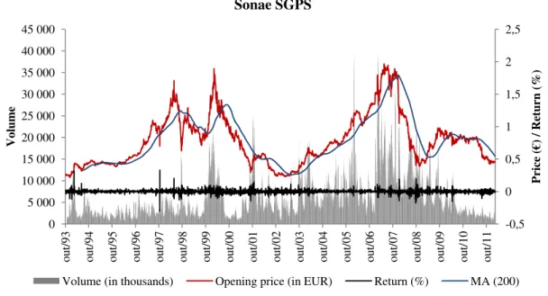
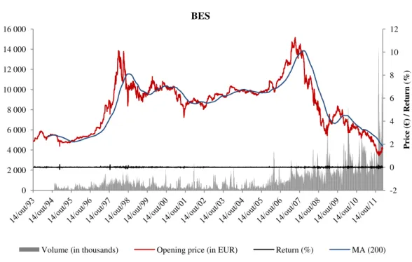
Through chart observation, one can find some relation between stock price moves, or returns, and volume, as is the case of Sonae SGPS presented in Figure 1 (see Figures A.1 to A.9 in the appendix for the other stocks). However, adding the 200-day moving average indicator does not appear to bring additional explanatory power. Nevertheless, it is important to study if there is any effect in volume if applying these trading rules, as so many traders actually use them.

FIGURE 1: STOCK PRICE, MOVING AVERAGE, RETURN AND VOLUME OF SONAE SGPS

0 5 000 10 000 15 000 20 000 25 000 30 000 35 000 40 000 45 000

out/93 out/94 out/95 out/96 out/97 out/98 out/99 out/00 out/01 out/02 out/03 out/04 out/05 out/06 out/07 out/08 out/09 out/10 out/11

-0,5 0 0,5 1 1,5 2 2,5

Volume

Price

(€) / Return

(%

)

Sonae SGPS

14

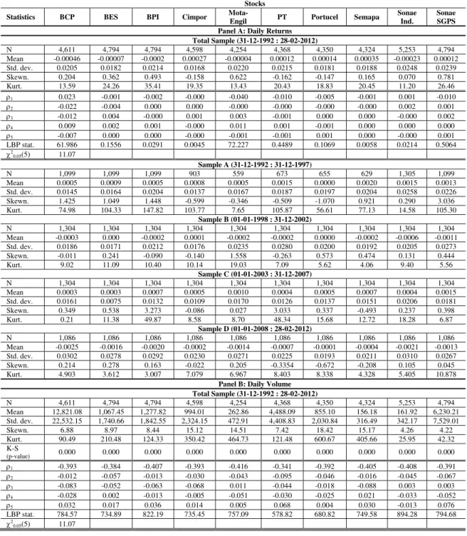
The summary statistics of the daily unconditional returns and volume for the 10 stocks that survived the filtering process are presented in Table I. We will call this unconditional mean return, the “buy-and-hold” (unconditional) strategy, which can be seen in the line Mean of Table I. Returns are calculated as log differences of stocks prices. Volume, the number of stocks traded, is presented in thousands. Panel A shows the descriptive statistics for daily returns. Although performances can range from -0.00046 (BCP) to 0.00035 (Semapa), the overall (average) return is null. All stocks show some evidence of skewness and excess kurtosis. Volatility is higher for Sonae Indústria (Sonae Ind.) that also witnessed the second worst performance and presents the less skewed and leptokurtic distribution. The information can also be observed in the four nonoverlapping subsamples mentioned before. A few words are worth to be outlined from here. In one hand, the first subsample, Sample A, is clearly not normally distributed what might be an expected characteristic of the years corresponding to the beginning of the market in Portugal. On the other hand, the four subsamples follow what apparently look as different cycles, or trends, if we look at the returns mean, and what could be empirically observed from the previously mentioned figures shown in the appendix. Sample A data is marked by a “bullish” market, while the data in Sample B seem to suggest an inversion to a “bearish” market, and the pattern repeats in the following two samples (Samples C and D are again “bullish” and “bearish”, respectively).

15

Blume et al. (1994) have previously stated that the volume statistic is not normally distributed. Sonae Indústria is the stock with the highest number of observations in the raw data as well as the less skewed and leptokurtic volume distribution.

TABLE I: SUMMARY STATISTICS FOR DAILY RETURNS AND VOLUME

Descriptive statistics and Kolmogorov-Smirnov (K-S) test for normality of each 10 stocks resulting from the filtering process. N is the number of days with available price and volume data for each stock. Mean and Std. dev. represent the mean and standard deviation of price returns and volume for each stock. Skewn. and Kurt. are respectively skewness and kurtosis of price returns and volume distributions of each stock. The first five autocorrelations of each stock are given by 1,...,5. Autocorrelations for volume

are measured using the differenced log volume series. LBP stat. refers to the Ljung-Box-Pierce statistic and it is distributed 2(5) under the null hypothesis of identical and independent distribution. K-S (p-value) shows the p-value of the hypothesis in the Kolmogorov-Smirnov test that volume is normally distributed. Panel A presents the descriptive statistics for daily returns. The information in Panel A is divided into five data samples (Total Sample and Samples A, B, C and D). The corresponding statistics for volume are shown in Panel B.

Stocks

Statistics BCP BES BPI Cimpor Mota-_Engil PT Portucel Semapa Sonae _Ind. Sonae _SGPS

Panel A: Daily Returns Total Sample (31-12-1992 : 28-02-2012)

N 4,611 4,794 4,794 4,598 4,254 4,368 4,350 4,324 5,253 4,794 Mean -0.00046 -0.00007 -0.0002 0.00027 -0.00004 0.00012 0.00014 0.00035 -0.00023 0.00012 Std. dev. 0.0205 0.0182 0.0214 0.0168 0.0220 0.0215 0.0181 0.0188 0.0248 0.0239 Skewn. 0.204 0.362 0.493 -0.158 0.622 -0.162 -0.147 0.165 0.070 0.781 Kurt. 13.59 24.26 35.41 19.35 13.43 20.43 18.83 20.45 11.20 26.46

1 0.023 -0.001 -0.002 -0.000 -0.040 -0.010 -0.005 -0.001 0.001 -0.010

2 -0.022 -0.004 0.000 0.000 -0.000 -0.000 -0.000 -0.000 0.002 0.001

3 -0.012 0.004 -0.000 0.001 0.003 -0.001 0.000 0.000 -0.000 0.002

4 0.009 0.002 0.001 -0.000 0.011 0.001 -0.001 0.000 0.000 0.000

5 -0.007 0.000 0.000 -0.000 -0.001 -0.001 0.001 0.000 -0.000 0.001

LBP stat. 61.986 0.1556 0.0291 0.0045 72.227 0.4489 0.1069 0.0058 0.0214 0.5064

2

0.05(5) 11.07

Sample A (31-12-1992 : 31-12-1997)

N 1,099 1,099 1,099 903 559 673 655 629 1,305 1,099 Mean 0.0005 0.0009 0.0005 0.0008 0.0005 0.0015 0.0000 0.0020 0.0015 0.0013 Std. dev. 0.0145 0.0164 0.0204 0.0137 0.0167 0.0187 0.0197 0.0204 0.0258 0.0226 Skewn. 1.425 1.049 1.448 -0.599 -0.346 -0.509 -1.070 0.921 0.290 3.036 Kurt. 74.98 104.33 147.82 103.77 7.65 105.87 56.61 77.13 14.58 105.30

Sample B (01-01-1998 : 31-12-2002)

N 1,304 1,304 1,304 1,304 1,304 1,304 1,304 1,304 1,304 1,304 Mean -0.0003 0.000 -0.0002 0.0001 -0.0002 -0.0002 0.0000 -0.0002 -0.0006 -0.0011 Std. dev. 0.0186 0.0171 0.0212 0.0176 0.0235 0.0280 0.0200 0.0192 0.0205 0.0273 Skewn. -0.011 0.241 -0.090 -0.140 1.558 -0.263 0.573 0.474 0.131 0.444 Kurt. 9.02 11.09 10.40 10.14 19.03 7.09 5.62 4.06 9.40 5.56

Sample C (01-01-2003 : 31-12-2007)

N 1,304 1,304 1,304 1,304 1,304 1,304 1,304 1,304 1,304 1,304 Mean 0.0003 0.0003 0.0007 0.0005 0.0010 0.0004 0.0005 0.0007 0.0004 0.0015 Std. dev. 0.0161 0.0075 0.0132 0.0109 0.0170 0.0126 0.0137 0.0151 0.0206 0.0181 Skewn. 0.349 0.538 3.273 -0.086 0.027 3.033 0.337 -0.493 0.237 0.398 Kurt. 0.21 11.38 49.87 8.58 8.70 48.34 15.68 12.72 18.28 6.87

Sample D (01-01-2008 : 28-02-2012)

N 1,086 1,086 1,086 1,086 1,086 1,086 1,086 1,086 1,086 1,086 Mean -0.0025 -0.0016 -0.0020 -0.0002 -0.0014 -0.0007 -0.0001 -0.0004 -0.0021 -0.0013 Std. dev. 0.0302 0.0278 0.0292 0.0230 0.0271 0.0225 0.0193 0.0211 0.0310 0.0267 Skewn. 0.214 0.278 0.163 -0.022 0.205 -0.3354 -0.672 -0.208 0.105 0.045 Kurt. 4.903 3.612 3.007 7.079 6.967 8.403 8.338 4.328 5.405 10.878

Panel B: Daily Volume Total Sample (31-12-1992 : 28-02-2012)

N 4,611 4,794 4,794 4,598 4,254 4,368 4,350 4,324 5,253 4,794 Mean 12,821.08 1,067.45 1,277.82 994.01 262.86 4,488.09 855.10 156.18 161.92 6,230.21 Std. dev. 22,532.15 1,740.66 1,842.55 2,324.15 472.91 4,408.83 2,030.84 316.49 342.17 7,529.01 Skewn. 6.88 8.97 8.44 15.12 14.51 7.42 18.42 15.17 4.26 4.22 Kurt. 90.49 210.48 124.33 350.42 464.73 121.48 600.67 405.66 25.95 42.32 K-S

(p-value) 0.000 0.000 0.000 0.000 0.000 0.000 0.000 0.000 0.000 0.000

1 -0.393 -0.384 -0.407 -0.393 -0.416 -0.341 -0.392 -0.405 -0.408 -0.391

2 -0.012 -0.057 -0.013 -0.030 -0.043 -0.095 -0.046 -0.016 -0.045 -0.067

3 -0.083 -0.052 -0.063 -0.068 0.011 -0.044 -0.018 -0.088 0.003 0.003

4 -0.028 0.002 -0.013 -0.005 -0.051 -0.030 -0.025 0.021 -0.033 -0.052

5 0.032 0.017 0.036 0.014 0.005 0.068 0.004 0.030 -0.013 0.076

LBP stat. 784.57 734.89 822.19 735.45 757.09 578.82 680.82 749.58 894.28 794.68

2

16

From the observation of the autocorrelation list, one can conclude that returns have no significant autocorrelations. On the other hand, the volume series (we use the differenced log volumes to obtain a stationary series) show significant autocorrelations in the first lag and that all stocks give strong rejection of the null hypothesis of identical and independent observations.

The analysis of Panel B data, suggests the use of nonparametric tests where no distribution is assumed (distribution-free) because the corresponding parametric tests are not applicable in this case as the volume distribution is clearly not normal. In particular, the Mann-Whitney statistic will be used to test the hypothesis that the medians of buys and sells are different. In this statistic, equal distributions between two independent populations are assumed, no matter the distribution format. To test for equal distributions between the two populations, the equivalent nonparametric Levene’s test is used. The formulation of this statistic is explained below. This will bring robustness of results for statistical inference.

3.2.METHODOLOGY

17

∑ where is the stock price for day t-i (1)

Once the day-to-day fluctuations are removed and a trend can be outlined, the rule can be used to help determine an uptrend or a downtrend if both price and a relevant moving average are used. Another method of determining momentum is to look at the cross of a pair of (unweighted) moving averages: a short period average and a long period average. This rule is an important method to identify buy and sell signals. When the short period average crosses the long period average from below (above), commonly called a golden (death) cross, the trend is up and it suggests a buy (sell) signal. In other words, the trading rule is to hold a long position when the difference between the short-term and the long-short-term moving average is positive, and to hold a short position otherwise.

To implement this strategies, a few of the most popular moving averages were built over the price series for each stock, with 2, 5, 50, 150 and 200 days lag, to build the moving average rules tested in the work of Brock et al. (1992), without the 1% bandwidth because there were no evidence of additional effectiveness in introducing the band. The rules differ by the length of the short and the long periods. The notation used is 1-50, 1-150, 5-150, 1-200 and 2-200, for the five rules constructed, where the first digit is the number of days of the short period and the latter ones are the number of days for the long period. Brock et al. (1992) state that the 1-200 moving average rule is the most broadly used, where the moving average pair 1 day and 200 days, for the short period and the long period, respectively, is used to identify signals.

18

signal is generated and is identified as “1”, and “-1” otherwise. From this rule, two groups are created, whether they are buys or sells, depending on the relative position of the moving averages.

In order to compare this five moving average strategies to the “buy-and-hold” (unconditional) strategy, we first run t-tests for the difference of the mean buy and mean sell returns from the “buy-and-hold” (unconditional) daily mean return (presented in Table I) and buy-sell from zero, for each stock. We then apply the strategy attempting to replicate a real investment according to both the “buy-and-hold” strategy and the trading rule described above. The former consists of buying the stock in the first trading day and holding it until the last trading day, then selling it. The latter assumes holding a long position as long as a buy signal is returned while in the case of a sell signal the shares are sold out and the trader waits until a new buy signal is received (we have not considered the investment in the risk-free asset or transaction costs). The profit analysis takes an initial investment of 1 € for both strategies, to simplify, and applies to the whole data sample. This approach intends to confirm whether the conclusions of the previous statistical tests are robust or not.

19

As presented in the previous section, the analysis of the raw data in Table I, suggested the use of nonparametric tests because the corresponding parametric tests are not applicable in this case as the volume distribution is not normal. The Mann-Whitney U test2 is used to investigate whether median volume of buys is statistically higher (lower) than median volume of sells. The equivalent nonparametric Levene’s test3 for equal variances, without assuming that groups are normally distributed is used to test homogeneity of variances between the ranked groups used in the Mann-Whitney U test and it brings additional robustness by confirming (or not) the groups have equal distributions. This conclusion is important to assess the validity of the first assumption of equal distributions between the two groups investigated in the Mann-Whitney U test. This statistic is computed as a one-way ANOVA over the absolute deviation of the population rank, independently of the groups, and the mean of the ranked population separated by the groups, according to the following expression:

, 1, 2, … , and , (2)

Finally, we entail an analysis of the correlation between prices (returns) and volume, using price moving average signals from one trading strategy as well as volume and one-day-lag volume interacted with one-day-lag returns, following the approach by Campbell et al. (1993), using the regression below:

(1)

2

Mann and Whitney (1947).

3

20

The signals resulting from the daily moving average rule on prices are included as an independent variable and take the values “1” or “0”, whether they are buys or sells, respectively. This methodology tries to replicate the strategy where we buy once a buy signal is generated and hold a long position until a sell signal is shown, then sell when a sell signal is presented and stay out of the market until a new buy signal is returned. Moreover, we need to work with stationary series so we use the first difference log volume series, in accordance to the same authors. Finally, we also need a measure of stock return volatility. To accomplish that, we compare the results using the generalized autoregressive conditional heteroskedasticity (GARCH(1,1)) and the exponential generalized autoregressive conditional heteroskedasticity (EGARCH(1,1)) and select the one that best fits the model, according to the minimum method selection criterion. The reason to consider an EGARCH along with the standard GARCH model relies on the fact that the former allows negative returns to increase volatility more than the positive ones.

4. RESULTS ANALYSIS

4.1.THE PRICE MOVING AVERAGE STRATEGY

21

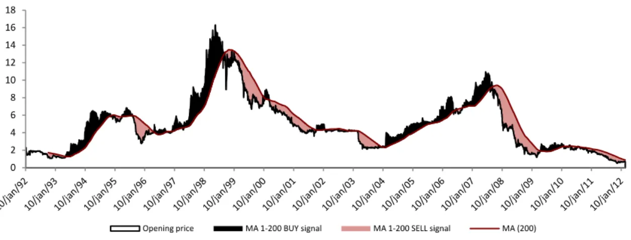
FIGURE 2: THE 1-200 MOVING AVERAGE STRATEGY EXAMPLE FOR SONAE INDÚSTRIA

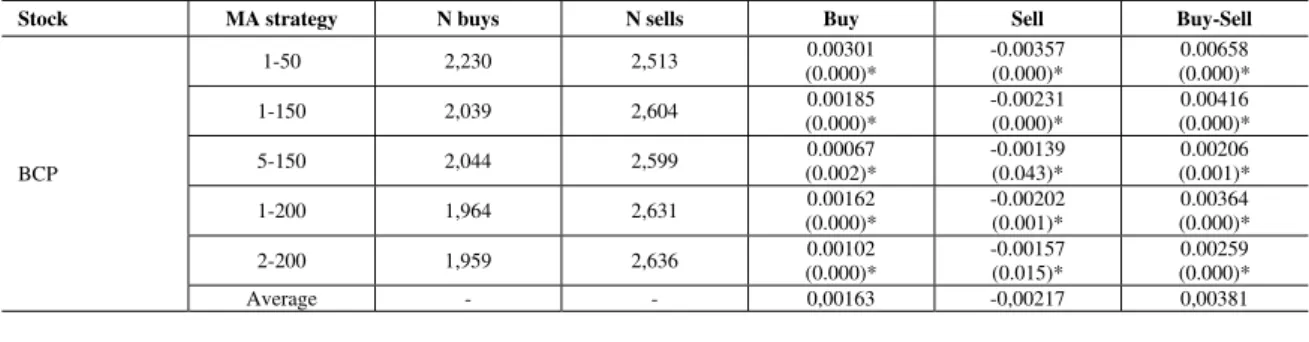
Table II reports the daily returns of both buy and sell periods replicated by the strategy above for each pair of moving averages (named “MA strategy” hereafter), and the corresponding p-values resulting from the t-tests for the difference of the mean buy and mean sell returns from the “buy-and-hold” (unconditional) daily mean return (presented in Table I) and buy-sell from zero4, for each stock. The number of signals generated by each strategy, whether they are buys or sells, is showed in column N total. N buys and N sells state respectively the number of buy and sell signals resulting from the moving average strategies listed in the MA strategy column for each stock.

4

The t-statistics for the buys (sells) are the ones used by Brock et al. (1992),

, (3)

where and are the mean buy (sell) return and number of buy (sell) signals, and µ and N are the

unconditional mean return and number of observations. is the estimated variance for the whole

sample. In the case of buy-sell, the t-statistic is,

, (4)

where and are respectively the mean return and number of buy signals, and and are the mean

return and the number of sell signals.

0 2 4 6 8 10 12 14 16 18

22

The results in Table II show that for all stocks buy returns (presented in column 5) are, on average, statistically higher than the “buy-and-hold” (unconditional) one-day return. Considering the results individually, the conclusion holds for almost all the strategies, except for a few cases. Additionally, the differences between the mean buy and mean sell returns listed in the last column show that they are all positive and the t -tests for these differences are highly statistically significant, rejecting the null hypothesis of equality of means at the 5% level, except for two cases, Portugal Telecom and Portucel, where the differences from mean buy and mean sell returns for the 5-150 moving average strategy are not statistically different from zero. Not surprisingly, the one sample t-tests for the buys in the cases mentioned above do not reject also the null hypothesis that the mean buy return is equal to the “buy-and-hold” (unconditional) one-day mean return. It is important to note also that in 5 out of 10 stocks, the p-values of the t-tests of the 5-150 moving average strategy show that the difference between mean buys and (or) mean sells are not statistically significant from the simple “buy-and-hold” (unconditional) one-day mean return presented in Table I, suggesting this moving average strategy does not appear to be a good trading strategy as no additional return can be obtained.

TABLE II: TEST RESULTS ON RETURNS FOR THE MOVING AVERAGE RULES

Results for daily data from inception date in the stock market to 28 February 2012, for each stock. Rules are shown according to the notation “short-long” to define the moving average (MA) strategy with a short period and a long period moving average, respectively. N buys and N sells are the number of buy and sell signals generated during the period. In Buy and Sell columns, each cell contains the respective mean return per strategy for each stock and, in brackets, the corresponding p-value of the t-test for the difference of the mean buy and mean sell from the “buy-and-hold” (unconditional) one-day mean presented in Table I. Buy-Sell shows the difference between columns Buy and Sell and the p-value of the t-test for the equality of means below, testing the difference (buy-sell) from zero. Numbers marked with an asterisk are statistically significant at the 5% level for a two-tailed test.

Stock MA strategy N buys N sells Buy Sell Buy-Sell

BCP

1-50 2,230 2,513 0.00301 (0.000)*

-0.00357 (0.000)*

0.00658 (0.000)* 1-150 2,039 2,604 0.00185

(0.000)*

-0.00231 (0.000)*

0.00416 (0.000)* 5-150 2,044 2,599 0.00067

(0.002)*

-0.00139 (0.043)*

0.00206 (0.001)* 1-200 1,964 2,631 0.00162

(0.000)*

-0.00202 (0.001)*

0.00364 (0.000)* 2-200 1,959 2,636 0.00102

(0.000)*

-0.00157 (0.015)*

0.00259 (0.000)*

23 BES

1-50 2,484 2,261 0.00267 (0.000)*

-0.00009 (0.936)

0.00276 (0.000)* 1-150 2,378 2,334 0.00118

(0.000)*

-0.00171 (0.000)*

0.00289 (0.000)* 5-150 2,298 2,347 0.00070

(0.005)*

-0.00090 (0.074)

0.00160 (0.003)* 1-200 2,301 2,294 0,00136

(0.000)*

-0.00159 (0.001)*

0.00295 (0.000)* 2-200 2,293 2,302 0.00093

(0.000)*

-0.00114 (0.022)*

0.00207 (0.000)*

Average - - 0,00137 -0,00109 0,00245

BPI

1-50 2,458 2,287 0.00311 (0.000)*

-0.00379 (0.000)*

0.00690 (0.000)* 1-150 2,486 2,334 0.00126

(0.000)*

-0.00233 (0.000)*

0.00359 (0.000)* 5-150 2,312 2,333 0.00091

(0.004)*

-0.00129 (0.030)*

0.00220 (0.001)* 1-200 2,307 2,288 0.00171

(0.000)*

-0.00201 (0.001)*

0.00372 (0.000)* 2-200 2,301 2,293 0.00142

(0.000)*

-0.00143 (0.016)*

0.00285 (0.000)*

Average - - 0,00168 -0,00217 0,00385

Cimpor

1-50 2,593 1,955 0.00262 (0.000)*

-0.00283 (0.000)*

0.00515 (0.000)* 1-150 2,728 1,721 0.00165

(0.000)*

-0.00189 (0.000)*

0.00354 (0.000)* 5-150 2,729 1,719 0.00073

(0.100)

-0.00043 (0.157)

0.00116 (0.028)* 1-200 2,711 1,688 0.00158

(0.000)*

-0.00182 (0.000)*

0.00340 (0.000)* 2-200 2,710 1,689 0.00092

(0.022)*

-0.00075 (0.040)*

0.00167 (0.002)*

Average - - 0,00150 -0,00154 0,00298

Mota-Engil

1-50 2,074 2,130 0.00379 (0.000)*

-0.00376 (0.000)*

0.00755 (0.000)* 1-150 2,275 1,829 0.00207

(0.000)*

-0.00264 (0.000)*

0.00471 (0.000)* 5-150 2,290 1,814 0.00120

(0.002)*

-0.00158 (0.012)*

0.00278 (0.000)* 1-200 2,237 1,817 0.00187

(0.000)*

-0.00236 (0.000)*

0.00423 (0.000)* 2-200 2,229 1,826 0.00132

(0.001)*

-0.00167 (0.007)*

0.00299 (0.000)*

Average - - 0,00205 -0,00240 0,00445

PT

1-50 2,325 1,994 0.00328 (0.000)*

-0.00354 (0.000)*

0.00682 (0.000)* 1-150 2,438 1,781 0.00232

(0.000)*

-0.00284 (0.000)*

0.00516 (0.000)* 5-150 2,417 1,802 0.00037

(0.628)

-0.00016 (0.562)

0.00053 (0.436) 1-200 2,423 1,746 0.00195

(0.000)*

-0.00250 (0.000)*

0.00445 (0.000)* 2-200 2,436 1,733 0.00085

(0.066)

-0.00099 (0.067)

0.00184 (0.008)*

Average - - 0,00175 -0,00201 0,00376

Portucel

1-50 2,323 1,976 0.00279 (0.000)*

-0.00297 (0.000)*

0.00576 (0.000)* 1-150 2,480 1,721 0.00172

(0.000)*

-0.00201 (0.000)*

0.00373 (0.000)* 5-150 2,481 1,720 0.00063

(0.124)

-0.00046 (0.241)*

0.00109 (0.057) 1-200 2,430 1,867 0.00153

(0.000)*

-0.00091 (0.033)*

0.00244 (0.000)* 2-200 2,429 1,721 0.00079

(0.038)*

-0.00065 (0.122)

0.00144 (0.011)*

Average - - 0,00149 -0,00140 0,00289

Semapa

1-50 2,425 1,848 0.00327 (0.000)*

-0.00354 (0.000)*

0.00681 (0.000)* 1-150 2,527 1,648 0.00194

(0.000)*

-0.00220 (0.000)*

0.00414 (0.000)* 5-150 2,519 1,656 0.00094

(0.067)

-0.00066 (0.066)

0.00160 (0.007)* 1-200 2,600 1,525 0.00169

(0.000)*

-0.00208 (0.000)*

0.00377 (0.000)* 2-200 2,591 1,534 0.00113

(0.014)*

-0.00111 (0.013)*

0.00224 (0.000)*

Average - - 0,00179 -0,00192 0,00371

Sonae Ind.

1-50 2,425 2,778 0.00424 (0.000)*

-0.00407 (0.000)*

0.00831 (0.000)* 1-150 2,304 2,800 0.00281

(0.000)*

-0.00263 (0.000)*

0.00544 (0.000)* 5-150 2,322 2,782 0.00170

(0.000)*

-0.00174 (0.002)*

24

The sells are all negative and fall below the “buy-and-hold” (unconditional) one-day mean return, except for a few cases where the mean sell returns are not statistically different from the unconditional mean return, assuming a 5% level two-tailed test. In the case of Banco Espírito Santo (BES), although the number of sell signals resulted from the 1-50 moving average strategy was almost twice the number of buys, the mean sell return is not statistically different from the unconditional mean of -0.007 per cent (see Table I), as the p-value is very high.

A separate analysis was conducted for each of the subsamples (see Table A.1 to A.4 of the appendix) and the conclusions are quite similar to the total sample ones. Please note that for Sample A, showing the most volatile distribution of returns due to including the inception and less liquid market period, the test results do not allow a conclusion on the strategies efficiency. All the other subsamples suggest consistent conclusions with the total sample results where nearly all stocks show that using the 5-150 moving average strategy does not allow a higher return than the unconditional strategy. This is also true for the 2-200 moving average rule, where at least 9 out of 10 stocks have no statistical difference between conditional and unconditional returns. In addition, the difference between buy and sell average returns are all positive (except for two cases in the 5-150 moving average rule of Portugal Telecom stock) and statistically different from zero.

1-200 2,306 2,748 0.00227 (0.000)*

-0.00213 (0.000)*

0.00440 (0.000)* 2-200 2,295 2,759 0.00178

(0.000)*

-0.00171 (0.002)*

0.00349 (0.000)*

Average - - 0,00256 -0,00246 0,00502

Sonae SGPS

1-50 2,546 2,199 0.00358 (0.000)*

-0.00387 (0.000)*

0.00745 (0.000)* 1-150 2,489 2,156 0.00257

(0.000)*

-0.00288 (0.000)*

0.00545 (0.000)* 5-150 2,464 2,181 0.00120

(0.004)*

-0.00127 (0.019)*

0.00247 (0.000)* 1-200 2,665 1,930 0.00200

(0.000)*

-0.00265 (0.000)*

0.00465 (0.000)* 2-200 2,665 1,930 0.00144

(0.000)*

-0.00187 (0.002)*

0.00331 (0.000)*

25

4.2.THE STRATEGY IN PRACTICE

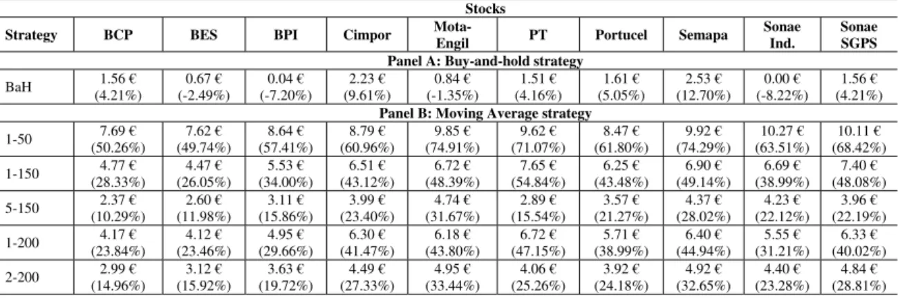
The trading accuracy of these moving average strategies can be better understood when comparing profits between these and the simple buy-and-hold strategy. While the former explore the strategy where we buy shares upon a buy signal and sell them upon a sell signal, the latter consists in buying shares in the first day the share went in the market and sell them in the last trading day of the sample. Table III presents the results of the comparison between the strategies for all ten stocks. Each cell contains two levels of information: first, the final value of the 1 € invested, and second, the annual return correspondent to the profit or loss over the period. Panel A shows the results for the simple buy-and-hold strategy. The profits for the five moving average strategies studied are presented in Panel B.

The results in Table III are striking. The profit gained in any moving average strategy is very much higher than in the buy-and-hold strategy. In fact, the latter experiences a loss in some of the stocks. These results seem to suggest that additional profits are able to get if we follow a technical rule such as the one behind the moving average strategies studied. Once again, in the results for Sonae Indústria lies a particular case as the stock

TABLE III: COMPARISON BETWEEN BUY-AND-HOLD AND MOVING AVERAGE STRATEGIES

Final value of the initial investment of 1 € and annual return correspondent to the profit or loss over the period, in brackets below, for every stock. Column Strategy defines the strategy adopted for each line of results, where BaH corresponds to the buy-and-hold strategy presented in Panel A. The results for the moving average strategies are presented in Panel B. Buy-and-hold explores the following strategy: we buy in the first day the stock went in the market and sell in the last trading day of the sample. Moving average strategies follows the rule: (1) buy shares upon a buy signal and hold a long position as long as a buy signal is returned and (2) sell upon a sell signal and wait (no investment in the risk-free asset or transaction costs) until a new buy signal is received.

Stocks

Strategy BCP BES BPI Cimpor Mota-_Engil PT Portucel Semapa Sonae _Ind. Sonae _SGPS

Panel A: Buy-and-hold strategy

BaH 1.56 € (4.21%) 0.67 € (-2.49%) 0.04 € (-7.20%) 2.23 € (9.61%) 0.84 € (-1.35%) 1.51 € (4.16%) 1.61 € (5.05%) 2.53 € (12.70%) 0.00 € (-8.22%) 1.56 € (4.21%)

Panel B: Moving Average strategy

1-50 7.69 € (50.26%) 7.62 € (49.74%) 8.64 € (57.41%) 8.79 € (60.96%) 9.85 € (74.91%) 9.62 € (71.07%) 8.47 € (61.80%) 9.92 € (74.29%) 10.27 € (63.51%) 10.11 € (68.42%) 1-150 4.77 €

(28.33%) 4.47 € (26.05%) 5.53 € (34.00%) 6.51 € (43.12%) 6.72 € (48.39%) 7.65 € (54.84%) 6.25 € (43.48%) 6.90 € (49.14%) 6.69 € (38.99%) 7.40 € (48.08%) 5-150 2.37 €

(10.29%) 2.60 € (11.98%) 3.11 € (15.86%) 3.99 € (23.40%) 4.74 € (31.67%) 2.89 € (15.54%) 3.57 € (21.27%) 4.37 € (28.02%) 4.23 € (22.12%) 3.96 € (22.19%) 1-200 4.17 €

(23.84%) 4.12 € (23.46%) 4.95 € (29.66%) 6.30 € (41.47%) 6.18 € (43.80%) 6.72 € (47.15%) 5.71 € (38.99%) 6.40 € (44.94%) 5.55 € (31.21%) 6.33 € (40.02%) 2-200 2.99 €

26

performance forces the trader, in the case of the buy-and-hold strategy, to completely lose his investment even before reaching the last trading day in the sample. However, if we consider the 1-50 moving average strategy for this same stock, the highest profit is observed, with the trader who invested 1 € in the first day that the stock came into the market ending up with a 10.27 € profit, before transaction costs, which corresponds to a 63.51% annual rate. Overall, the results range from 0.00 € (buy-and-hold strategy - Sonae Indústria) to 10.27 € (1-50 moving average strategy - Sonae Indústria).

4.3.THE CASE OF VOLUME

After analysing the results of the t-tests on daily returns, it is interesting to look at the behaviour on volume to understand if there is any reaction to the buy and sell signals of the moving average strategy on prices. In particular, we are interested to study if trading volume is higher on buy periods (after a buy signal) than on sell periods (after a sell signal).

27

groups are normally distributed. The F-statistic of the one-way ANOVA and the p-value (in brackets) are displayed in the last column of Table III.

The results are consistent with the results presented in Table II. The median volumes of buys statistically different from the median volumes of sells result from moving average strategies where the mean buy returns are statistically different from the mean sell returns. Nevertheless, the results are not quite revealing of a general statistical difference between buy and sell group volumes. This may happen because the Portuguese stock market has still received little attention and study, rather than the Dow Jones or Nasdaq indices in the United States. However, there are some quite interesting results to point out as they may support some of Brock et al. (1992) conclusions. If we look at the Mann-Whitney U test column, even though in the majority of the strategies the null hypothesis cannot be rejected, a few strategies have resulted in a statistical difference between the medians of both groups. If we look at the p-values of some strategies (asterisk marks they are statistically significant) we can say, because we have reasons to believe in that, the median buy volume in a given moving average strategy is statistically higher (lower) than the median sell volume, based on the Mann-Whitney U test. The equivalent nonparametric Levene’s test assesses the robustness of the Mann-Whitney U results by testing the homogeneity of variances between the groups i.e. if both groups have the same distribution. The null hypothesis in the equivalent nonparametric Levene’s test is rejected in only two of the fifty statistical tests in Table II (and only marginally significant in a third one), with p-values below a 5% significance level, which supports the statistical inference power of the previous test.

28

volume is statistically higher than the median buy volume, in the case of BCP. Only in BCP we can conclude that the mean volume is higher in a bearish market than in a bullish one. For all the other stocks where the differences are statistically different, the results show that the mean volume is higher in an up-trended market (buys) than in a downtrend (sells). In the 1-50 strategy, the results for BES and BPI are only marginally statistical significant, though for Semapa and Sonae Indústria the median difference is highly significant and we may say the median buy volume is statistically higher than the median sell volume in these four stocks. The previous conclusion stands even though the equivalent nonparametric Levene’s test for Semapa being only marginally significant what may decrease the supporting strength to the Mann-Whitney U test in this case. Mota-Engil is the only stock where the results on volumes are fully consistent with Brock et al. (1992) conclusions on returns: higher median and more volatile volume in buys than in sells, if we look at the 2-200 moving average strategy test. Another important fact to state is that there is only statistical evidence of different behaviour in volume in three strategies: 1-50, 1-200 and 2-200. These may actually be the strategies traders are using to trace price trends and identify momentum in Portuguese stocks in the PSI 20. The 1-200 moving average strategy was actually what the previous authors said to be the most popular trading rule amongst practitioners.

TABLE IV: RESULTS OF NONPARAMETRIC TESTS OVER VOLUME DISTRIBUTION

Results for daily volume data from inception date in the stock market to 28 February 2012, for each stock. Volume is given by the number of shares traded. Rules are shown according to the notation “short-long” to define the moving average (MA) strategy with a short period and a long period moving average, respectively. The number of signals generated over the entire sample is shown in column N total. N buys and N sells are the number of buy and sell signals generated during the period. Median (buys) and Median (sells) represent the median of each stock Volume distribution. Mann-Whitney and Nonparametric Levene’s test columns contain, at a first level, the t-statistics of the Mann-Whitney U test and the equivalent nonparametric Levene’s test for the equality of means, and the p-value of the previous t-statistics in brackets below. Numbers in the Mann-Whitney U (nonparametric Levene’s) test column marked with one (two) asterisk(s) are statistically significant, or marginally, at the 5% level for a 1-tailed test.

Stock _strategy MA _total N _buys N _sells N Median _(buys) Median _(sells) Mann-Whitney Nonparametric Levene’s test

BCP

1-50 158 78 80 4 545,05 4 411,80 3 063 (0,422)

0,456 (0,500)** 1-150 69 33 36 4 328,80 6 291,45 549

(0,298)

0,065 (0,800)** 5-150 46 23 23 5 905,80 8 117 246

(0,348)

29

1-200 71 38 33 2 909,05 8 165,25 446 (0,018)*

0,097 (0,756)** 2-200 64 34 30 3 107,85 9 527,05 363

(0,024)*

0,146 (0,704)**

BES

1-50 163 88 75 631,50 366,20 2 816 (0,054)*

0,875 (0,351)** 1-150 74 41 33 484,10 753,30 579,5

(0,147)

2,319 (0,132)** 5-150 54 28 26 461,80 790,55 335

(0,312)

0,188 (0,667)** 1-200 59 29 30 371,60 359,50 417

(0,396)

2,116 (0,151)** 2-200 49 24 25 368,80 330,60 284

(0,379)

1,881 (0,177)**

BPI

1-50 165 77 88 961,70 831,70 2 903 (0,057)*

0,005 (0,945)** 1-150 73 36 37 1 184,20 919,10 624

(0,323)

0,051 (0,822)** 5-150 48 22 26 1 590,50 879,95 226

(0,110)

0,094 (0,761)** 1-200 58 30 28 1 241,20 1 146,60 352

(0,148)

0,010 (0,919)** 2-200 47 27 20 974,70 923 252

(0,355)

0,983 (0,327)**

Cimpor

1-50 206 104 102 463,15 370,10 4 667,5 (0,069)

0,072 (0,789)** 1-150 101 52 49 497,85 426,70 1 249

(0,434)

0,071 (0,790)** 5-150 57 29 28 353,30 373,45 392

(0,415)

0,010 (0,922)** 1-200 83 47 36 424,40 381,35 723,5

(0,131)

2,011 (0,160)** 2-200 71 38 33 328,25 308,90 576

(0,281)

2,239 (0,139)**

Mota-Engil

1-50 146 86 60 150,05 114,95 2 467 (0,327)

9,869 (0,002) 1-150 63 29 34 33,70 90,65 458

(0,317)

5,929 (0,018) 5-150 38 19 19 42,00 39,10 169

(0,373)

0,336 (0,566)** 1-200 51 26 25 77,85 40,30 254

(0,092)

1,889 (0,176)** 2-200 43 17 26 160,60 27,40 152,5

(0,045)*

0,164 (0,687)**

PT

1-50 161 86 75 4 896,40 4 936 2 994 (0,218)

0,774 (0,380)** 1-150 97 42 55 4 990,65 5 818,80 1 127

(0,421)

0,13 (0,719)** 5-150 60 27 33 5 415,90 6 184,40 420

(0,356)

0,163 (0,688)** 1-200 85 36 49 5 702,45 5 579,20 879

(0,4919

1,227 (0,271)** 2-200 68 30 38 5 898,45 5 634,55 544

(0,377)

0,243 (0,623)**

Portucel

1-50 148 78 70 406,85 436 2 586 (0,291)

0,647 (0,423)** 1-150 69 43 26 649,10 399,95 473

(0,146)

2,116 (0,150)** 5-150 47 24 23 694,05 408,10 222

(0,129)

0,009 (0,925)** 1-200 61 35 26 550,30 403,55 406

(0,241)

0,143 (0,707)** 2-200 50 25 25 567,70 535 300

(0,409)

0,094 (0,760)**

Semapa

1-50 166 86 80 105,10 73,30 2 898,5 (0,040)*

3,673 (0,057) 1-150 69 36 33 67,95 94,50 529

(0,220)

0,639 (0,427)** 5-150 50 27 23 115 166 297

(0,399)

2,471 (0,123)** 1-200 51 25 26 142,60 71,90 240

(0,056)*

0,215 (0,645)** 2-200 47 20 27 109,40 76 231,5

(0,207)

2,310 (0,136)**

Sonae Ind.

1-50 162 81 81 69,20 29,40 2 694 (0,025)*

0,037 (0,847)** 1-150 61 30 31 79,65 31,50 369

(0,085)

0,379 (0,541)** 5-150 39 23 16 37,20 14,45 158

(0,233)

0,444 (0,510)** 1-200 46 27 19 78,40 117,30 255

(0,491)

0,233 (0,632)** 2-200 37 21 16 109 181,35 161

(0,422)

30

4.4.REGRESSION ANALYSIS

The previous tests have shown some statistical evidence of different behaviors between buy and sell periods following price moving average rules signals. These differences are seen both in prices and volumes. It is then important to investigate the correlation between prices and volume by regressing price moving average and volume on return.

The model is defined by the following equation, according to Campbell et al. (1993), using daily price moving average signals, volume and one-day-lag volume interacted with one-day-lag returns as regressors to explain individual stock price returns:

(5)

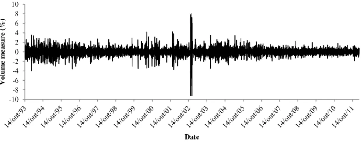
We consider the series of the 1-200 moving average rule signals as it is referenced to be the most popular one and returned consistent results in the statistical testing. In order to work with stationary time series in our empirical study, we use the 1st difference log volume series, similarly to Campbell et al. (1993). Figure 3 shows the stationary volume series (see Figure A.10 in the appendix for the raw series), taking the example of BCP. Sonae SGPS

1-50 132 66 66 4 266,35 4 331,10 2 126 (0,408)

0,044 (0,835)** 1-150 87 47 40 4 561,60 5 040,15 868

(0,272)

0,085 (0,772)** 5-150 57 27 30 5 546,50 4 763,90 356

(0,221)

0,001 (0,974)** 1-200 61 30 31 5 824,50 4 023,60 417

(0,248)

1,074 (0,304)**

2-200 55 23 32 4 785,80 3 684,25 345 (0,352)

31

FIGURE 3: STATIONARY LOG TURNOVER SERIES, TOTAL SAMPLE

Our transformed series show no trend signs. Finally, to measure stock return volatility we compare the results using a generalized autoregressive heteroskedasticity (GARCH(1,1)) and the exponential generalized autoregressive heteroskedasticity (EGARCH(1,1)). These models allow us to correct the residual autocorrelation. The EGARCH differs from the standard GARCH model by allowing negative returns to increase volatility more than the positive ones. Both models use minimum likelihood method estimation. The model is selected according to the minimum method selection criterion and only that one is presented in Table V. Asterisk marks the use of EGARCH instead of GARCH model.

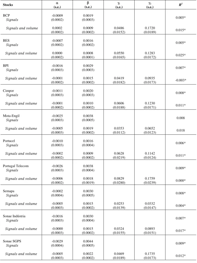
Table V presents the coefficients of the regression of current stock return on the moving average signals as well as the current and last day volume interacted with one-day-lag stock return. We conduct two separate analyses: first, we regress current stock return on the moving average signals; and second, an alternative regression includes the current volume and lagged volume interacted with the last day stock return. Results in Table V are based on the total sample.

-10 -8 -6 -4 -2 0 2 4 6 8 10

V

ol

ume

me

as

ur

e (

%

)

Date

32

TABLE V: REGRESSION ON MOVING AVERAGE SIGNALS AND VOLUME INTERACTED WITH PAST RETURN

Each stock of the list in the column Stocks has two lines presenting the coefficients of two regressions on current return in accordance to the equation above. The four following columns show respectively the coefficients of the constant, the 1-200 moving average rule signal, the current volume interacted with the one-day-lag stock return and the one-day-lag volume interacted with the one-day-lag stock return. The volume series is presented in log differences. Last column is the R2 _{statistic of the regression in the}

respective line. The values marked with an asterisk show the R2 of the regression using the EGARCH instead of the GARCH model.

Stocks  (s.e.)



(s.e.) (s.e.) (s.e.) R2

BCP -0.0009

(0.0002) 0.0002 (0.0002) 0.0019 (0.0003) 0.0009 (0.0002) 0.0486 (0.0152) 0.1720 (0.0189) 0.005* 0.015*

BES -0.0007

(0.0002) 0.0000 (0.0002) 0.0016 (0.0002) 0.0008 (0.0001) 0.0550 (0.0165) 0.1283 (0.0172) 0.005* 0.025* BPI -0.0016 (0.0003) -0.0001 (0.0002) 0.0029 (0.0003) 0.0015 (0.0002) 0.0419 (0.0182) 0.0935 (0.0173) 0.007* -0.003* Cimpor -0.0011 (0.0003) -0.0001 (0.0002) 0.0020 (0.0003) 0.0010 (0.0002) 0.0606 (0.0188) 0.1230 (0.0171) 0.008* 0.011* Mota-Engil -0.0025 (0.0003) -0.0005 (0.0003) 0.0038 (0.0005) 0.0019 (0.0002) 0.0353 (0.0112) 0.0652 (0.0123) 0.008 0.018 Portucel -0.0010 (0.0003) -0.0002 (0.0002) 0.0016 (0.0004) 0.0009 (0.0002) 0.0628 (0.0219) 0.1142 (0.0124) 0.006* 0.011*

Portugal Telecom -0.0026

(0.0003) -0.0006 (0.0002) 0.0038 (0.0004) 0.0018 (0.0019) 0.0829 (0.0280) 0.1759 (0.0239) 0.009* 0.000*

Semapa -0.0002

(0.0004) -0.0005 (0.0003) 0.0030 (0.0005) 0.0015 (0.0002) 0.0253 (0.0139) 0.0332 (0.0147) 0.008* 0.004*

Sonae Indústria -0.0016

(0.0003) -0.0000 (0.0003) 0.0030 (0.0004) 0.0015 (0.0002) 0.0324 (0.0155) 0.0893 (0.0151) 0.007* 0.017*

Sonae SGPS -0.0029

33

The first line of all stocks in Table V shows that at least 0.5% of the variance of each current stock return can be explained by a regression on current moving average signal. The R2 statistics for these regressions are low, ranging from 0.5% to 0.9%. It is also true that for all stocks, except for three, the R2 increases (and in some cases more than doubles) once the interaction between volume and one-day-lag return is included. In this case, the statistic may come up to 2.5%. These results can be seen in the second line of each stock. All regressors are always statistically significant at the 5% level.

Not surprisingly, besides increasing the explanatory power of current stock return, coefficients of volume are consistently positive in influencing the dependent variable. The one-day-lag volume interacted with the one-day-lag return is the regressor taking the principal part in changing the expected stock return.

5. CONCLUSIONS, LIMITATIONS AND FUTURE INVESTIGATION

34

This conclusion comes first from the parametric tests run on price returns of individual stocks, where we followed the methodology suggested by Brock et al. (1992) and found that for all stocks, returns conditional on buy signals are, on average, statistically higher than the unconditional one-day return and that the differences between mean buy and mean sell returns are all positive and statistically significant, rejecting the null hypothesis of equality of means at the 5% level, except for a few cases. Additionally, we applied the strategy by simulating a real investment following the price moving average strategy and compare it to the simple buy-and-hold strategy. While the former allows consistent and significant profits for all stocks and all moving average rules, the latter one has a low performance and actually brings to a loss in 40% of them, considering the available data sample of about 20 years back from 28 February 2012.

In the case of volume, no general conclusion of an empirical relationship between price moving average rules and this variable was found on our investigation though in some particular stocks the results from the nonparametric tests suggests that following price moving average signals the median volume of buys is statistically different from the median volume of sells in three out of five rules. As said before, when included in a regression on returns, the variables have got little explanatory power, for it cannot offer significant support to the empirical tests run before this analysis. Volume and one-day-lag volume, though, interacted with the one-day-one-day-lag return regressors can actually double the R2 of the regression (though it was able to deliver R2 of only 2.5%) from what it was if the regression included only the price moving average signals as independent variable.

35

conclusions above. Firstly, we did not consider any transaction costs when simulating the returns of the strategies in Chapter 2, what is not realistic as a trader or investor would have to pay commissions or brokerage fees whenever they buy or sell the stocks. In addition, we decided to use parametric tests over distributions that were not clearly normal. It does not seem to be a very problematic choice because the distribution of returns suggests only slight non-normality and in reality one cannot expect to obtain a perfectly normal distribution.

We suggest those who think in pursuing further investigation in this issue to take into account the transaction costs and brokerage fees in the performance analysis, as well as study different and more elaborate rules and test their effectiveness.

36 REFERENCES

Alexander, S. S. (1961). Price movements in Speculative Markets: Trends or Random Walks. Industrial Management Review 2, 7-26.

Alexander S. S. (1964). Price movements in Speculative Markets: Trends or Random Walks, No. 2. Industrial Management Review 5, 25-46.

Blume, Easley, D. and O’Hara, M. (1994). Market Statistics and Technical Analysis: The Role of Volume. The Journal of Finance 49 (1), 153-181.

Brock, Lakonishok, J. and LeBaron, B. (1992). Simple Technical Trading Rules and the Stochastic Properties of Stock Returns. The Journal of Finance 47 (5), 1731-1764.

Brown, D. P. and Jennings, R. H. (1989). On Technical Analysis. The Review of Financial Studies 2 (4), 527-551.

Campbell, Grossman, S. J. and Wang, J. (1993). Trading Volume and Serial Correlation in Stock Returns. The Quarterly Journal of Economics 108 (4), 905-939.

Fama, E. F. (1970). Efficient Capital Markets: A Review of Theory and Empirical Work. The Journal of Finance 25 (2), 383-417.

Fama, E. F. and Blume, M. E. (1966). Filter Rules and Stock-Market Trading. The Journal of Business 39 (1), 226-241.

Gençay, R. and Stengos, T. (1998). Moving Average Rules, Volume and the Predictability of Security Returns with Feedforward Networks. Journal of Forecasting

37

Gervais, Kaniel, R. and Mingelgrin, D. H. (2001). The High-Volume Return Premium.

The Journal of Finance 56 (3), 877-919.

Goldberg, M. and Schulmeister, S. (1988). Technical Analysis And Stock Market Efficiency. Working Papers 88-21. C.V. Starr Center for Applied Economics, New York University.

Kavajecz, K. A. and Odders-White, E. R. (2004). Technical Analysis and Liquidity Provision. The Review of Financial Studies 17 (4), 1043-1071.

Lo, Mamaysky, H. and Wang, J. (2000). Foundations of Technical Analysis: Computational Algorithms, Statistical Inference, and Empirical Implementation. The Journal of Finance 55 (4), 1705-1765.

Mann, H. B. and Whitney, D. R. (1947). On a Test of Whether one of Two Random Variables is Stochastically Larger than the Other. The Annals of Mathematical Statistics

18 (1), 50-60.

Neftci, S. N. (1991). Naïve Trading Rules in Financial Markets and Wiener-Kolmogorov Prediction Theory: A Study of “Technical Analysis”. The Journal of Business 64 (4), 549-571.

Peña, D. (2005). Análisis de Series Temporales, Madrid: Alianza Editorial.

Ramachandran, K. M. and Tsokos, C. P. (2009). Mathematical Statistics with Applications, 1st Edition Elsevier Academic Press.

38 APPENDIX

FIGURE A.1: STOCK PRICE, MOVING AVERAGE, RETURN AND VOLUME OF BANCO COMERCIAL PORTUGUÊS

FIGURE A.2: STOCK PRICE, MOVING AVERAGE, RETURN AND VOLUME OF BANCO ESPÍRITO SANTO

0 100 000 200 000 300 000 400 000 500 000 600 000

-1 0 1 2 3 4 5

Volum

e

Price

(€

) / Return (%

)

BCP

Volume (in thousands) Opening price (in EUR) Return (%) MA (200)

0 2 000 4 000 6 000 8 000 10 000 12 000 14 000 16 000

-2 0 2 4 6 8 10 12

Volum

e

Price

(€

) / Return (%

)

BES

39

FIGURE A.3: STOCK PRICE, MOVING AVERAGE, RETURN AND VOLUME OF BANCO BPI

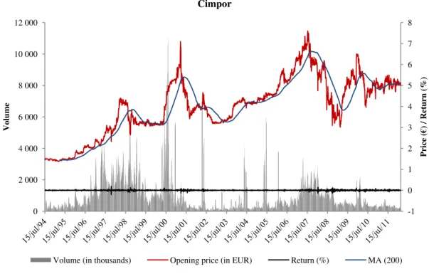
FIGURE A.4: STOCK PRICE, MOVING AVERAGE, RETURN AND VOLUME OF CIMPOR

0 2 000 4 000 6 000 8 000 10 000 12 000 14 000 16 000 18 000

-1 0 1 2 3 4 5 6 7

Volum

e

Price

(€

) / Return (%

)

Banco BPI

Volume (in thousands) Opening price (in EUR) Return (%) MA (200)

0 2 000 4 000 6 000 8 000 10 000 12 000

-1 0 1 2 3 4 5 6 7 8

Volum

e

Price

(€

) / Return (%

)

Cimpor

40

FIGURE A.5: STOCK PRICE, MOVING AVERAGE, RETURN AND VOLUME OF MOTA-ENGIL

FIGURE A.6: STOCK PRICE, MOVING AVERAGE, RETURN AND VOLUME OF PORTUGAL TELECOM

0 500 1 000 1 500 2 000 2 500 3 000 3 500

-1 0 1 2 3 4 5 6 7 8 9

Volum

e

Price

(€

) / Return (%

)

Mota-Engil SGPS

Volume (in thousands) Opening price (in EUR) Return (%) MA (200)

0 5 000 10 000 15 000 20 000 25 000 30 000

-2 0 2 4 6 8 10 12 14 16

Volum

e

Price

(€

) / Return (%

)

PT

41

FIGURE A.7: STOCK PRICE, MOVING AVERAGE, RETURN AND VOLUME OF PORTUCEL

FIGURE A.8: STOCK PRICE, MOVING AVERAGE, RETURN AND VOLUME OF SEMAPA

0 2 000 4 000 6 000 8 000 10 000 12 000 14 000

-0,5 0 0,5 1 1,5 2 2,5 3 3,5

Volum

e

Price

(€

) / Return (%

)

Portucel

Volume (in thousands) Opening price (in EUR) Return (%) MA (200)

0 200 400 600 800 1 000 1 200 1 400 1 600

-2 0 2 4 6 8 10 12 14 16

Volum

e

Price

(€

) / Return (%

)

Semapa

42

FIGURE A.9: STOCK PRICE, MOVING AVERAGE, RETURN AND VOLUME OF SONAE INDÚSTRIA

FIGURE A.10: LEVEL OF BCP STOCK VOLUME, TOTAL SAMPLE

0 500 1 000 1 500 2 000 2 500

-2 0 2 4 6 8 10 12 14 16 18

Volum

e

Price

(€

) / Return (%

)

Sonae Indústria

Volume (in thousands) Opening price (in EUR) Return (%) MA (200)

0 100 000 200 000 300 000 400 000 500 000

Volum

e (in

thousands)

Date

43

TABLE A.1: SUBSAMPLE A - TEST RESULTS ON RETURNS FOR THE MOVING AVERAGE RULES

Results for daily data for subsample A, for each stock. Rules are shown according to the notation “short-long” to define the moving average (MA) strategy with a short period and a long period moving average, respectively. N buys and N sells are the number of buy and sell signals generated during the period. In Buy and Sell columns, each cell contains the respective mean return per strategy for each stock and, in brackets, the corresponding p-value of the t-test for the difference of the mean buy and mean sell from the unconditional one-day mean presented in Table I. Buy-Sell shows the difference between columns Buy and Sell and the p-value of the t-test for the equality of means below, testing the difference (buy-sell) from zero. Numbers marked with an asterisk are statistically significant at the 5% level for a two-tailed test.

Stock MA strategy N buys N sells Buy Sell Buy-Sell

BCP

1-50 591 459 0.0025

(0.001)*

-0.0023 (0.000)*

0.0048 (0.000)*

1-150 485 465 0.0022

(0.015)*

-0.0013 (0.005)*

0.0035 (0.000)*

5-150 490 460 0.0014

(0.246)

-0.0005 (0.059)

0.0019 (0.049)*

1-200 448 453 0.0018

(0.141)

-0.0005 (0.038)*

0.0023 (0.023)*

2-200 445 456 0.0016

(0.200)

-0.0003 (0.090)

0.0019 (0.054)

Average - - 0,0019 -0,0010 0,0029

BES

1-50 742 309 0.0024

(0.001)*

-0.0029 (0.004)*

0.0053 (0.000)*

1-150 685 271 0.0015

(0.302)

-0.0010 (0.155)

0.0025 (0.079)

5-150 675 276 0.0014

(0.394)

-0.0006 (0.269)

0.0020 (0.176)

1-200 674 227 0.0016

(0.232)

-0.0013 (0.147)

0.0029 (0.030)*

2-200 673 228 0.0014

(0.376)

-0.0007 (0.277)

0.0021 (0.103)

Average - - 0,0017 -0,0013 0,0030

BPI

1-50 636 415 0.0034

(0.000)*

-0.0040 (0.000)*

0.0074 (0.000)*

1-150 555 414 0.0017

(0.252)

-0.0022 (0.012)*

0.0039 (0.000)*

5-150 532 419 0.0014

(0.405)

-0.0003 (0.285)

0.0017 (0.228)

1-200 512 389 0.0028

(0.013)*

-0.0014 (0.077)

0.0042 (0.003)*

2-200 509 392 0.0018

(0.244)

-0.0001 (0.394)

0.0019 (0.183)

Average - - 0,0022 -0,0016 0,0038

Cimpor

1-50 531 324 0.0023

(0.001)*

-0.0015 (0.020)*

0.0038 (0.000)*

1-150 1252 76 0.0019

(0.013)*

-0.0039 (0.101)

0.0058 (0.002)*

5-150 679 76 0.0009

(0.806)

0.0012 (0.675)

-0.0003 (0.879)

1-200 683 22 0.0014

(0.192)

-0.0124 (0.178)

0.0138 (0.159)

2-200 684 21 0.0011

(0.625)

-0.0014 (0.332)

0.0025 (0.446)

Average - - 0,0015 -0,0036 0,0051

Mota-Engil

1-50 302 209 0.0026

(0.017)*

-0.0025 (0.020)*

0.0051 (0.001)*

1-150 338 73 0.0019

(0.114)

-0.0048 (0.045)*

0.0067 (0.017)*

5-150 342 69 0.0015

(0.277)

-0.0030 (0.204)

0.0045 (0.124)

1-200 312 49 0.0016

(0.258)

-0.0039 (0.238)

0.0055 (0.154)

2-200 312 49 0.0016

(0.258)

-0.0039 (0.238)

0.0055 (0.154)

Average - - 0,0018 -0,0036 0,0055

Portucel

1-50 328 279 0.0027

(0.001)*

-0.0031 (0.037)*

0.0058 (0.000)*

1-150 330 177 0.0021

(0.044)*

-0.0029 (0.109)

0.0050 (0.010)*

5-150 328 179 0.0003

(0.770)

0.0005 (0.775)

-0.0002 (0.934)

1-200 299 220 0.0020

(0.079)

-0.0008 (0.641)

0.0028 (0.024)*

2-200 298 159 0.0010

(0.272)

-0.0006 (0.788)

0.0016 (0.433)

Average - - 0,0016 -0,0014 0,0030

Portugal Telecom

1-50 490 135 0.0028

(0.022)*

-0.0022 (0.201)

0.0050 (0.007)*

1-150 518 7 0.0027

(0.117)

-0.0381 (0.333)