Structured Products in the Current Low Interest Rate Environment

(1)

A Work Project presented as part of the requirements for the Award of a Masters Degree in Finance from NOVA School of Business and Economics

Directed Research Internship

Structured Products in the Current Low Interest Rate

Environment

João Francisco Teles de Freitas Saldanha, 734

Abstract

This study presents an analysis on the Portuguese market of structured products and the

features used to mitigate the problem of the current low interest rates. Given the

possible combinations, it proposes a specific product that enables an annualized yield of

4.5% to the investor if his expectations materialize during the next 2 years, while

providing the issuer with a 2% upfront commercial margin.

It also addresses some of the risks for the issuer of such product and the magnitude of

their impact in the hedging process.

Keywords: Structured Products, Auto-Callable, Worst of Digital

A Project carried out under the supervision of Professor Afonso Eça

(2)

2

Table of Contents

Introduction ... 3

The Portuguese Market ofStructuredProducts ... 4

1. Features used in the Portuguese Market ... 4

2. The Proposed Structure ... 7

3. The Chosen Underlying ... 9

Auto-Callable Worst of Digital ... 11

1. Methodology ... 11

2. The Quote ... 14

3. Hedging Process ... 16

4. Other Risks to the Issuer ... 18

4.1. Unhedgeable Deltas due to liquidity constraints... 19

4.2. Gap Risk ... 20

4.3. Vega vs. Correlation Vega ... 21

Conclusion ... 22

References ... 24

(3)

3

Introduction

Structured products were created to enable financial institutions address the different

needs of their clients. Due to their customizable characteristics, these products can be

designed either for hedging purposes or for speculation, taking always into account the

risk profile of each investor.

A structured financial product can be seen as a bundle of different financial assets which

put together create a desired payoff. Financial institutions sell these to their clients and,

simultaneously, hedge themselves through a back-to-back transaction, which means

buying the same product from another issuer. However, when they believe it is more

efficient, they can replicate these products in the market by hedging each source of

uncertainty. In either way, the profit of the institution is independent of the product’s

payoff and the price of the underlying.

One example of a structured product is a capital guaranteed investment that at maturity

pays the notional back plus a return that is dependent on the value of the underlying.

This kind of structured product can for example be replicated by buying a zero-coupon

bond with the same maturity and notional and using the remaining funds (funding) to

buy derivatives on the underlying asset.

However, recently, a problem arose in the Portuguese market of capital guaranteed

structured products. When the interest rates fell to historical lows, offering attractive

products started being difficult because funding ceased to cover the price of the required

derivatives.

So, how can financial institutions enhance the yield of its structured products in the

current low interest rate environment? There are limited ways to achieve this, thus the

purpose of this study will be to analyze the options available in the market and propose

(4)

4

while respecting the commercial constrains. Afterwards, it will address the main issues

of issuing such product, addressing the risks for the issuer and the impact of each

variable considered when quoting and hedging this product.

The Portuguese Market ofStructuredProducts

The purpose of this study is to propose a retail structured product to sell to clients that is

still attractive even during the current low interest rate period. In order to choose the

best structure that, simultaneously, takes into account the profile of the targeted

investors and the current problem of low funding, it is important to understand how

each Portuguese financial institution is overcoming the problem and analyze each

option.

To do it, this study compiled all the retail structured products offered in Portugal, which

are registered either with CMVM or Bank of Portugal since the beginning of 2014 (a

total of 220 products), and extensively analyzed the characteristics embedded in each

one that enabled the creation of a product with the required level of attractiveness.

Subsequently, and after weighting the advantages and disadvantages of each option, it

presents a final structure with the characteristics that best respond to the problem.

1. Features used in the Portuguese Market

The right structure is the key piece to increase commercial attractiveness while

constrained by the low interest rates. Through the analysis of the Portuguese market,

one can conclude that, in order to overcome the problem of lack of funding, an issuer

can either: increase the maturity, add capital risk, cap the gain, make the payoff in the

form of a conditional coupon or use other features to decrease the cost of the structure.

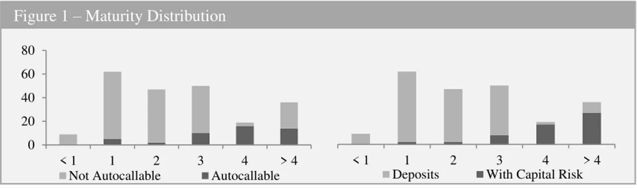
Regarding maturity, figure 1 illustrates that most products (159) have maturities from

(5)

5

maturities and because timeframes longer than 3 years might exceed investors’ macro

expectations’ scope. A common solution to mitigate these constraints is the inclusion of

an auto-callable feature that introduces the possibility of an earlier maturity.

Adding capital risk can be accomplished by embedding into the structure a short

derivative (e.g. a put option). This way, the investor acts like the underwriter of that

component, using the proceeds to finance the rest of the structure. One problem with

adding capital risk results from the fact that structured products are a particularly good

asset for very risk-averse investors to buy in order to get exposure to financial markets

without endangering their initial capital. Besides lowering the number of potential

investors, having capital risk on a product in Portugal makes it unable to have the

denomination of a deposit and therefore, stops being guaranteed by the Deposit

Guarantee Fund, which, given the current Portuguese environment, might weigh on the

investors’ decisions. As can be perceived in figure 1, products with capital risk usually

have higher maturities because they are usually bought by the same, less risk-averse,

investors.

Figure 2 - With or Without Risk Figure 1 – Maturity Distribution

< 1 1 2 3 4 > 4

Deposits With Capital Risk 0

20 40 60 80

< 1 1 2 3 4 > 4

Not Autocallable Autocallable

23,4%

76,6%

(6)

6

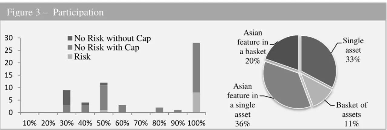
Some features can be added in order to create cheaper structures. These decrease the

value for the investor but try to maintain an attractive yield if market expectations are

met. Figure 3 illustrates some of the features that are added to a product in order to

increase the participation in the upside (for non-digital products). This can be done by

choosing underlyings with low volatilities, or choosing stocks with high dividend yield

or capping the gain at a certain level.

Regarding the underlying’s volatility, instead of directly choosing an asset with low

volatility, the issuer can choose a basket of low correlated assets or add an Asian

feature. The Asian feature, in practice, is the same as having a lower volatility because it

reduces the impact of a sudden price deviation.

One other alternative to increase the yield with the same funding is by replacing the

participation in the upside for a conditional fixed coupon. This way, the issuer can

increase the value of the coupon by lowering the mathematical probability of the

product actually paying it. Figure 4 proves that currently this option is being extensively

used. There are two effective ways to decrease this probability: one is to add a worst of

feature in a basket with low correlated assets, which will increase the probability of one

asset not following the other’s tendency and underperform, while the other option is to

make the conditional coupon subject to a knock-out American barrier. The latter is used,

for example, on range products, where the probability of underlying’s price never Figure 3 – Participation

0 5 10 15 20 25 30

10% 20% 30% 40% 50% 60% 70% 80% 90% 100% No Risk without Cap

(7)

7

breaching the barriers during the product’s life is substantially lower than the

probability of only requiring to be inside the range at maturity.

Regarding the chosen underlying’s asset class, this might have an impact on the cost of

the structure but then, its most important purpose is to increase the commercial

attractiveness of the product by being well-known and observable for the common

investor.

2. The Proposed Structure

After this extensive analysis of the already issued retail products, it is possible to

understand that the popularity of digital payoff is explained by their effectiveness in

overcoming the low interest rates problem. Designing a product paying large coupons

(even if with low mathematical probabilities of paying it) is the best option to enhance

the yield obtained from correct market expectations.

The possibility of not being capital guaranteed will be disregarded here, since it would

considerably decrease the targeted clients interested in this product. As can be perceived Figure 4 – Digital Options

Figure 5 –Underlying’ asset class

148 61

Digital Coupon Participation in upside

65% 31%

4%

Digital (american barrier)

Regular digital

Worst of digital 148

129

54

17 13 13 ₅

(8)

8

by the previous analysis, the common Portuguese investor might search for structured

products as an alternative to a low paying term deposit. However, he will still look for

the main characteristic of these popular deposits, which is having guaranteed capital

(which are even guaranteed by the Deposit Guarantee Fund).

On the other hand, in capital guaranteed products, using conditional coupons instead of

participations in the upside is not enough to finance high coupons; hence the structured

product must have a longer maturity. To keep from reducing the targeted investors, this

product will have a maturity of 2 year with an auto-callable feature every semester.

While the maturity of two years still allows for market expectations for that timeframe,

the auto-callable feature lowers the expected maturity. Additionally, an early maturity is

good for both the investor and the issuer since the first will retrieve its investment

earlier with the desired return and the latter will gain from the increasingly better

commercial relationship with their clients. Moreover, a worst of digital in a basket of

assets is the most effective structure to improve the control over the trade-off between a

high coupon and the probability of paying it. In this type of product, the issuer can

choose the number and the type of assets to include in the basket, giving him some

control over the initial probability of payment. Choosing low correlated assets or assets

paying high dividend yields are examples of methods to influence this probability.

Ultimately, the product will have the issuer’s desired combination between the coupon’s

amount and probability from the combinations allowed by this mathematical trade-off.

Table 1 - Summary of the Proposed Structure

Underlying: Basket of Assets

Maturiry 2 Years

Type of Payoff: Conditional Digital Coupon

Risk: Capital Guaranteed

Features included: Worst of

Autocallable Every Six months

(9)

9

3. The Chosen Underlying

Regarding the best asset class, this depends mostly on the targeted investors and their

specific needs. Given the objective of increasing the number of potential interested

investors, an easily understandable asset class must be chosen in order to mitigate the

already high complexity of such products. Therefore, the proposed asset class to include

as underlying is equity because it is easy to commercialize given its high level of

simplicity, liquidity and transparency.

It is in this stage of choosing the stocks that the issuer has the responsibility to add value

to the product that is not captured by the options models valuation. By making a

top-down analysis, starting with the development of macro expectations and then an

individual research on each company, the issuer increases the actual probability of

payment by using its expertise and knowledge to choose a promising industry and solid

single stocks. Thus, the resulting difference between the model probability of payment

and the actual probability will add value to the product and to the client without

jeopardizing the issuer’s commercial margin.

At the time of this report, it was in the author’s opinion that there was unpriced value in

the European utility sector. Given Europe’s borderline deflation and shy recovery, the

expectation of further expansionary policies from the European Central Bank (ECB)

made utilities a promising sector. Utility companies are characterized by high levels of

regulation and low cash flow volatility, which, combined with the necessary amount of

non-current fixed assets, lead to high levels of leverage. Thus, this asset class works as a

proxy to bonds since lower interest rates will boost earnings by decreasing the huge

interest weight. This characteristic makes this sector the perfect choice in the current

environment of low interest rates and therefore, is consistent with the objective of

(10)

10

Furthermore, this sector is known for its high dividend yields, which, besides increasing

its demand in low interest rate periods, will improve the possible offered quote for the

product. Additionally, given the exposure to country-specific regulatory changes, these

companies might present low correlations if their activities are based in different

countries.

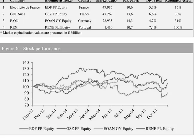
Regarding the single stocks chosen, a study on the existing European utility companies

was performed and 4 companies were chosen based on demonstrated stability, solid

operations and undervalued stock prices. Additionally, these companies had some

priced negative news-flow that was believed to be exaggerated, such as the impact of

the French Government desire to reduce nuclear power dependency to 50%, without

having any viable economic alternative and the Belgium nuclear tax that might be

considered illegal by the European Court of Justice. A summary of the 4 stocks and

their 52 weeks performance are presented in table 2 and figure 6, respectively.

i Company Bloomberg Ticker Country Market Cap.* P/E 2014E Div. Yield Regulated Assets

1 Electricite de France EDF FP Equity France 47.915 10,6 5,7% 15%

2 GDF Suez GSZ FP Equity France 47.262 13,6 6,6% 30%

3 E.ON EOAN GY Equity Germany 28.935 14,3 4,7% 31%

4 REN RENE PL Equity Portugal 1.410 10,7 7,4% 100%

* Market capitalization values are presented in € Million Table 2 – Stocks Chosen

~

(11)

11

Auto-Callable Worst of Digital

The product chosen is defined as a capital guaranteed Auto-callable (even though

normally these have capital risk) on a basket composed by 4 stocks. It has a maximum

maturity of 2 years with a possible conditional early maturity every six months. The

auto-callable barrier coincides with the coupon barrier, thus this product will terminate

earlier in the event a coupon is paid. The product is an Auto-callable with memory,

which means the coupon offered increases linearly with the number of semesters in

which there was no payment, thus maintaining a constant annualized rate independent

of the payment period. Appendix 1 illustrates this payoff through a timeline.

The pricing of such product is not straightforward given the discontinuous payoff and

unknown maturity. Deng, Mallett and McCann (2011) suggest a pricing formula based

on the Partial Differential Equation approach but it is only applied when the underlying

is a single asset. Since this product is a worstof on a basket of stocks, this option cannot

be applied.

The approach used in this study was suggested by Boyle (1977) and requires the

simulation of n sample price paths several times in the risk-neutral world (Monte Carlo

simulations) and the computation of the discounted payoff of the option for each path.

By relying on the law of large numbers, the average of these simulations will tend to the

true value of option. This method will be described in depth in the methodology.

The issuance of such product has some risks associated, which are listed in Fower and

Outgenza (2004) and will be further addressed in the section of other risks to the issuer.

1. Methodology

Given the unknown maturity and the path dependency of this product there is no

closed-form solution to price it and, therefore, the only way to do it is through the already

(12)

12

( 1 )

( 2 ) to execute this approach. This method required the simulation of 100.000 possible paths

or each asset price of the underlying basket in a risk neutral framework. The equation 11

is used to simulate the price for a Δt length of time,

𝑆𝑖(𝑡 + ∆𝑡) = 𝑆𝑖(𝑡) exp [(𝑟𝑓 − 𝑑𝑦𝑖 −𝜎𝑖

2

2 ) ∆𝑡 + 𝜀𝑖]

To generate 𝜀_𝑖, independent samples (𝑥_𝑖, 𝑥_𝑖+1 , ⋯ , 𝑥_𝑘, ⋯ , 𝑥_𝑛) are generated from n

independent standard normal distributions (where n is the number of assets in the

basket) and are then subject to a procedure known as the Cholesky decomposition,

which makes the n series of 𝜀correlated with each other according to their implied

correlations. This procedure is done by multiplying the vector 𝑥 (𝑥_𝑖, 𝑥_𝑖+1, ⋯ , 𝑥_𝑘, ⋯ ,

𝑥𝑛) by matrix 𝐴𝑇, which is computed from the implied covariance matrix (Ω) through

the equation,

Ω = 𝐴 ∙ 𝐴𝑇

After simulating the 100.000 different scenarios, the payoff and maturity of the product

in each one of these must be computed. The discounted average of the resulting payoffs

is the value of the product.The quote of the product, in this case the coupon, is defined

so that the value of the product matches the amount paid by the client less the issuer’s

commercial margin.

The reasoning behind this commercial margin is that the financial institution must

charge something for the service it is providing and for the risks and costs it is

incurring. This service includes, not only the advice regarding market expectations or

concerning the appropriate product for each risk profile, but also the commercial

1

where Si(t) is the price of asset i at time t, rf is the Euribor, dyi is the implied dividend yield of asset i, σi

(13)

13

relations with the product’s issuers. It also must charge the operational costs, the risks

that the issuer incurs in the issuance of such products and the costs with the

management of the dynamic hedging process necessary afterwards.

1.1.Inputs

Estimating the inputs required might be straightforward or not, depending on the

derivatives available in the market for the chosen stocks. Normally, the inputs that

might be implied in market prices are volatilities and dividends, which can be

extrapolated from options or dividend futures. When not available, volatilities can be

estimated through the existing models and the dividends through the company’s

dividend policy, history, operation results and the analysis of comparables. Appendix 2

and 3 summarize the inputs used in the simulations for the different tenors and stocks.

The challenge surfaces with the estimation of the future covariance matrix to use in the

pricing, which is not observable in market prices. Therefore, an issuer could choose to

ask for a quote on a correlation swap with a counterparty but, besides sometimes being

impossible, these might include a considerable premium due to the lack of liquidity of

these contracts.

So, a practical way to do this is by estimating the future correlation through the

historical correlation. However, as it will be addressed in the risk section, these inputs

are very volatile and have a significant weight in the product’s quote. Therefore, given

the normal difference between implied volatility and realized volatility, implied

correlations will also have a premium relative to the historical correlation, which in this

product will be set at 0.2, in order to make a conservative quoting and allow for a

(14)

14

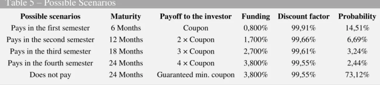
( 3 ) 2. The Quote

In order to price this product and provide a corresponding quote, it is necessary to

understand the possible scenarios and their corresponding probability.

There are 5 possible scenarios to the outcome of this product. The Monte Carlo

simulation enables the estimation of the probability of each one. These estimated

probabilities are the key output of the Monte Carlo simulation because with them the

issuer can easily price all simple variation of the simulated product.

Table 5 describes the five different possible scenarios and the corresponding

probabilities computed through the 100.000 simulations. The funding used here is the

deposit rates offered by Banco de Investimento Global (Banco BiG) for the different

tenors plus a small spread due to the fact that structured products usually have large

notionals, therefore attaining better rates.

With this information, through equation 3, the different possible quotes can be

computed for the issuer’s desired commercial margin. In this equation, i designates each

of the 5 possible scenarios described above with each corresponding probability

(𝑃𝑟𝑜𝑏_𝑖), funding (𝐹_𝑖) and discount factor (𝑑𝑓_𝑖).

∑[𝑃𝑟𝑜𝑏𝑖(𝐹𝑖 − 𝑃𝑎𝑦𝑜𝑓𝑓𝑖) × 𝑑𝑓𝑖]

5

𝑖=1

= 𝐶𝑜𝑚𝑚𝑒𝑟𝑐𝑖𝑎𝑙 𝑀𝑎𝑟𝑔𝑖𝑛

Regarding the desired commercial margin, this mostly depends on each bank’s position

in the trade-off between the product’s competitiveness and the contract’s profit margin. Possible scenarios Maturity Payoff to the investor Funding Discount factor Probability

Pays in the first semester 6 Months Coupon 0,800% 99,91% 14,51%

Pays in the second semester 12 Months 2 × Coupon 1,700% 99,66% 6,69%

Pays in the third semester 18 Months 3 × Coupon 2,700% 99,61% 3,24%

(15)

15

Even though each issuer has a reference margin, the latest structured products offered

by the competitors were priced, in order to understand which margin leads to a

competitive product in the Portuguese market. A total of 22 products were priced from 9

different banks, however, it is important to underline that the margins reached are not

each bank’s commercial margins but the margins that Banco BiG would get if it issued

each exact product. The difference comes from the fact that each bank has its inputs,

especially regarding their funding term structure that, for the purpose of comparing the

competitiveness between products, must be assumed the same for the different banks.

Appendix 4 presents the results from this product analysis and shows that, lately, the

average total commercial margin of the products offered in Portugal is 2.42% or 1.02%

per year. Hence, the proposed product will have a target commercial margin per year of

1%. This margin would make this product more competitive than the products of 5 of

the 9 banks analyzed.

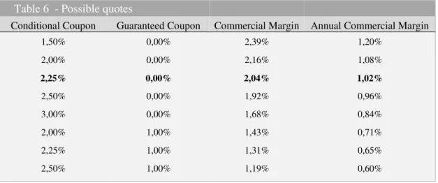
Finally, to quote this structured product, an analysis of the possible combinations

between the conditional coupon and the guaranteed minimum coupon must be

performed in order to know which combination could reach the desired commercial

margin. Table 6 summarizes these combinations, which were computed according with

equation 3.

Table 6 - Possible quotes

Conditional Coupon Guaranteed Coupon Commercial Margin Annual Commercial Margin

1,50% 0,00% 2,39% 1,20%

2,00% 0,00% 2,16% 1,08%

2,25% 0,00% 2,04% 1,02%

2,50% 0,00% 1,92% 0,96%

3,00% 0,00% 1,68% 0,84%

2,00% 1,00% 1,43% 0,71%

2,25% 1,00% 1,31% 0,65%

2,50% 1,00% 1,19% 0,60%

(16)

16

( 4 ) Thus, the final proposed product will pay a conditional coupon of 2.25% with no

minimum guaranteed coupon, which translates into a maximum annualized rate of

4.50% and a minimum of 0%. It will provide the issuer with an upfront commercial

margin of 2.04% at the time of the issuance.

3. Hedging Process

After selling this product, unless a back-to-back transaction takes place, the issuer will

need to manage his consequent position periodically. Such management will be

performed according to the sensitivity of the product to the various sources of

uncertainty, depending on its importance. These are represented through the different

sensitivity calculations, known as the Greeks.

Given the discontinuous payoff, a critical analysis to some of these Greek is required

because these might result in absurd or frequently changing values that would be

inefficient to hedge.

The Greeks were computed by the finite differencing method with the same 100.000

Monte-Carlo simulations. Equation 4 exemplifies this calculation for the delta of the

product according to the suggestion of Taleb (1996), which states that in discrete

changes, the impact of an increase in the spot price might not be the same as a decrease

of the same magnitude. In this case, the ∆𝑆_𝑖 used was 0.01 × 𝑆_𝑖. The resulting delta

represents the number of stocks required to replicate the issuer’s position.

𝐷𝑒𝑙𝑡𝑎𝑖 =𝑃𝑎𝑦𝑜𝑓𝑓(𝑆𝑖 + ∆𝑆𝑖) − 𝑃𝑎𝑦𝑜𝑓𝑓(𝑆_2∆𝑆 𝑖− ∆𝑆𝑖)

𝑖

The Deltas are the main measures computed and require an immediate offset. Besides

representing the main driver for the value of the product, their correct hedging aligns the

(17)

17

( 5 )

( 6 )

( 8 ) Gamma, which quantifies the sensitivity of Delta in EUR to a 1% change in the

underlying price, was computed according to the equation2,

𝐺𝑎𝑚𝑚𝑎𝑖 = 𝐷𝑒𝑙𝑡𝑎𝑖

∗_(𝑆

𝑖+ ∆𝑆𝑖) − 𝐷𝑒𝑙𝑡𝑎𝑖∗(𝑆𝑖− ∆𝑆𝑖)

2

Which is, approximately,

𝐺𝑎𝑚𝑚𝑎𝑖 = 𝑃𝑎𝑦𝑜𝑓𝑓(𝑆𝑖 + 2∆𝑆𝑖) + 𝑃𝑎𝑦𝑜𝑓𝑓(𝑆_{4 × 0.01}𝑖− 2∆𝑆𝑖) − 2 × 𝑃𝑎𝑦𝑜𝑓𝑓(𝑆𝑖)

Since the issuer undertakes the mandatory dynamic hedging, supposedly, the Gammas

of the product could be left hedged. However, in practice, because it is impossible to

perform continuous trading, there is a gap risk that will be addressed in the other risks

section.

Furthermore, a Greek which is not often computed but that in this kind of products is

very important is the Correlation Vega. This sensitivity calculation translates the impact

of a change in the correlation between the different pairs of assets in the basket, which

given the worst of feature, changes significantly the probability of paying the coupon,

and is calculated according with the equation,

𝐶𝑜𝑟𝑟𝑒𝑙𝑎𝑡𝑖𝑜𝑛 𝑉𝑒𝑔𝑎𝑖,𝑗 = 𝑃𝑎𝑦𝑜𝑓𝑓(𝜌𝑖𝑗+ ∆𝜌𝑖𝑗_{2 × 10}) − 𝑃𝑎𝑦𝑜𝑓𝑓(𝜌𝑖𝑗 − ∆𝜌𝑖𝑗)

By defining ∆𝜌_𝑖𝑗 = 0.1, the Correlation Vega measures the impact of a correlation

increase of one percentage point, between asset i and asset j, in the value of the product.

Regarding Theta, since this Greek accounts for the impact of the passage of time, there

is no use in measuring the impact of more time-to-maturity, only less. However, this

variation does not represent any uncertainty given the fact that the passage of time is

2

(18)

18

certain. Therefore, even though its value can change considerably, the computation of

this Greek is merely informative, given that the lack of uncertainty makes hedging the

impact of the passage of time an unnecessary labor.

The Greeks of this product at the time of the issuance are described in table 7. All

calculations were computed for a 1.000.000 € of notional.

Table 7 - Greeks

Stocks Delta Gamma Vega Overall Product Greeks

EDF -36.899 1.430 93 Theta -67

GSZ -17.414 2.167 42 Rho -180

EOAN -15.200 1.836 40 Vega 277

RENE -44.666 2.204 103 Correlation Vega -281

Pairs: EDF / GSZ EDF / EOAN EDF / RENE GSZ / EOAN GSZ / RENE EOAN / RENE

Correlation Vega -43 -28 -63 -70 -44 -36

* All values are in EUR

Thus, if no other hedge carried out besides a dynamic delta hedge, such position for the

issuer will mean a value decrease of 67€ per day, a decrease of 281€ for each

percentage point increase in the correlation between all assets and an estimated loss of

180€ for every 10 basis points increase of the interest rates. Alternatively, this product

contributes for the issuer being long on volatility (he gains 277€ if all assets’ volatility

increases by one percentage point), which is an uncommon position for issuers.

4. Other Risks to the Issuer

The possibility of having the price of the worst of stock (the stock with the worst

performance since the initial date) near its strike price close to an auto-callable date is

the main risk of issuing this kind of product.

When this situation happens, due to the discontinuous payoff, the delta of this stock

explodes to values which might not be feasible or efficient to hedge. Additionally, this

(19)

19

the Gap risk, and sometimes varies with magnitudes where the trading volumes of that

stock do not allow for the necessary hedging (liquidity constraints).

Besides these problems, this product has a correlation risk exposure that might

sometimes be underestimated by traders and lead to unpleasant surprises.

4.1.Unhedgeable Deltas due to liquidity constraints

Table 8 presents each stock’s Delta and Gamma for a scenario where all stock prices are

15% higher their initial price except for REN, which would be at-the-money. This

measures are computed for this scenario, two days before the second auto-callable date

(therefore in one year from now).

Table 8 - At-The-Money Greeks near an Auto-Callable Date

Stock in EUR Number of Shares Average Daily volume

Delta* Gamma* Delta Gamma

EDF -17.164 2.501 -658 103 1.368.345

GSZ -7.929 1.184 -378 60 5.798.758

EOAN -5.964 813 -403 59 8.894.507

RENE -1.096.621 38.862 -449.435 20.424 345.239

According to these values, the issuer will require a position of 1.096.621€ in REN for

every 1.000.000 € of notional placed, representing a position close to 110% of the

notional in one stock. Depending on the stock’s liquidity, it might be impossible to buy

such quantities in the necessary period since, for example, REN’s last month’s daily

average volume is 345.239 shares. This means that for a product with 3 million euros of

notional, a 2% price decrease in REN’s shares in this scenario would oblige the issuer to

buy almost 35% of the daily volume, according to the gamma computed. This could

have an impact in the stock price, which could lead to the actual hedging process to

sustain the price level at-the money until the product’s auto-callable date. Afterwards,

the issuer would need to sell this considerable position, which might be difficult to

(20)

20

Even if REN’s stock price ends up slightly lower than the strike price in this second

auto-callable date, its next day delta would drop to -144.347 ( 14,4% of the notional),

which would mean that the issuer would need to sell quickly 390.159 shares for every

million euros of notional of a stock that has an average daily volume of 345.239 shares.

Another situation that could happen when the hedging process has an impact on the

market prices due to low liquidity is unexpectedly higher deltas. A scenario where this

would happen is under similar circumstances to the ones described before but this time

with REN’s price 2% lower than its strike price. In such a scenario, REN’s delta and

gamma, resulting from this position, would be -456.425 € and -326.645€, respectively.

Therefore, a 1% increase in the stock price would compel the issuer to buy 133.195

shares of REN, representing again almost 40% of the daily volume. A situation such as

this would put a significant pressure in the stock price, driving its value even further up,

therefore increasing considerably the delta of this stock.

Normally, both these situations could be mitigated by buying Calls on the at-the-money

stock in order to leverage the position and, in the case of the second scenario, decrease

the gamma risk. However, this might be impossible to accomplish for some stocks like

REN, which do not have listed options.

4.2.Gap Risk

The gap risk exists due to the possible jumps in the underlying asset price at the opening

of the market or between rebalancing of deltas. This gap risk is especially important in

this product given the huge dynamics of delta when an auto-callable date is near. In

such a situation, a jump in the price of the underlying will change considerably the

product’s deltas and lead to profits / losses from the hedging process very different from

(21)

21

To exemplify the magnitude that this gap risk can reach, it is necessary to retrieve the

first situation where only REN was at-the-money two days before the auto-callable date.

Again, the issuer is holding a 1.096.621€ position in REN (for a €1 million of notional)

when REN’s price either opens 5% lower or it suddenly decreases 5% without the issuer

having the opportunity to rebalancing his position in between. In this situation, the

product value for the issuer will increase 24.444 € but it will lose 54.831 € in REN’s

position, therefore losing 30.387 € in the hedging process.

Thus, the Gamma might sometimes be left unhedged but issuers must understand when

its magnitude makes its offset mandatory.

4.3.Vega vs. Correlation Vega

Normally, when issuing options, one of the most important inputs is the implied

volatility and so this variable is closely followed by derivatives traders. However, in this

product, it is arguable which is more important: volatility or correlation. In case of a

Capital Guaranteed Auto-callableeach stock’s volatility loses gradually its importance

to the implied correlations with each asset added to the basket.

The Vega and Correlation Vega values computed show that accurate correlations’

estimates are at least as important as implied volatilities. Moreover, the similar

magnitude between these values also proves that, in order to improve the quote of the

project, choosing low correlated assets for the basket will be as significant as choosing

high volatility stocks.

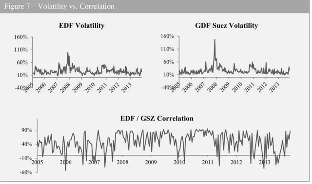
Furthermore, even though they present similar magnitudes, the volatility of the

volatilities is lower than the volatility of the correlations. Figure 7 presents this with the

computation of the series of correlation and volatilities for non-overlapping windows of

10 days for the stock price of EDF and GDF Suez. The difference between the standard

(22)

22

volatility series; therefore, the higher uncertainty in correlation makes the Correlation

Vega especially important.

Conclusion

The present study suggests capital guaranteed Auto-Callables as the products that

maximize commercial attractiveness in the current low interest rate environment. This

kind of product may be used to effectively enhance yield according to the market

expectations of the issuers and clients by using a cheap structure.

To issue such a product, the issuer at the initial date would unavoidably be required to

buy the computed deltas of each stock according with the notional placed, while

rebalancing this value periodically with a dynamic hedging process. The remaining

parameters may be left unhedged except for gamma when the product is at-the-money

near an auto-callable date, which leaves the issuer very exposed to market prices

variations, even if delta is hedged.

The main risks for the investors who buy this product are: market risk that is limited to

(23)

23

the market; credit risk that in this case is subject to Banco BiG’s creditworthiness; and

tax risk because the tax framework may change prior to maturity. It is also subject to

interest rate risk since its increase would lead to a lower present value of the coupons

and their decrease would make an early maturity less attractive since reinvestments at

the same rates would be difficult to accomplish.

When issuing this product, issuers must also understand the risks associated. These are,

mainly: the gap risk that exists because it is impossible to perform continuous trading,

and there are some situations where discrete trading might lead to considerable losses

for the issuer; and the possibility of having delta positions which are impossible or

inefficient to hedge due to liquidity constraints, in which case the hedging process can

even drive market prices against the issuer.

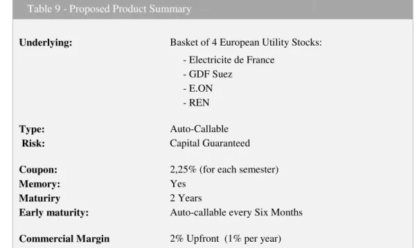
Thus, after acknowledging the risks associated, this report suggests the product

summarized in table 9 as a product that efficiently overcomes the problem of low

interest rates.

Table 9 - Proposed Product Summary

Underlying: Basket of 4 European Utility Stocks:

- Electricite de France

- GDF Suez

- E.ON

- REN

Type: Auto-Callable

Risk: Capital Guaranteed

Coupon: 2,25% (for each semester)

Memory: Yes

Maturiry 2 Years

Early maturity: Auto-callable every Six Months

Commercial Margin 2% Upfront (1% per year)

(24)

24

References

Banco de Portugal - Prospetos informativos de depósitos indexados e duais. 2014. Banco de Portugal.

http://clientebancario.bportugal.pt/pt-PT/ProdutosBancarios/ContasdeDeposito/Prospectosinformativos/Paginas/Prosp ectosinformativos.aspx

Boyle, Phelim. 1977. "Options: a Monte Carlo approach". Journal of Financial Economics, 4: 323-338.

Broadie, Mark, and Paul Glasserman. 1996. "Estimating Security Price Derivatives Using Simulation". Management Science, 42 (2): 269-285.

CMVM. 2009. "O Perfil do Investidor Particular Português".

http://www.cmvm.pt/cmvm/estudos/em%20arquivo/Pages/default.aspx

CMVM - Informação sobre Produtos Financeiros Complexos. 2014. CMVM -

Comissão do Mercado de Valores Mobiliários. http://web3.cmvm.pt/sdi2004/pfc/index_pfc.cfm

Deng, G., J. Mallett, and C. McCann. 2011. "Modeling Autocallable Structured Products". Journal of Derivatives & Hedge Funds, 17: 326-340

Fower, G., and L. Outgenza. 2004. "Auto-Callables: Understanding the products, the issuer hedging and the risks." Citigroup.

Glasserman, Paul. 2004. Monte Carlo Methods in Financial Engineering. New York: Springer Science + Business Media.

Hull, J. C. 2011. Options, Futures, and Other Derivatives.8th ed. New Jersey: Person Education.

SuperDerivatives. 2014. SuperDerivatives Inc. https://superderivatives.com/

(25)

25

Appendix

Appendix 2 – Current Euribor and Implied Volatility Appendix 3 – Dividend Yield

Tenor Euribor Implied Volatility Semester Estimated Annualized Dividend Yield

EDF GSZ EOAN RENE EDF GSZ EOAN RENE

15-05-2015 0,18% 22,3% 22,9% 23,6% 19,0% I 5,1% 5,5% 0,0% 10,7%

17-11-2015 0,34% 21,5% 22,5% 23,5% 19,2% II 5,0% 5,4% 6,8% 0,0%

16-05-2016 0,26% 21,3% 22,7% 22,9% 19,4% III 5,1% 5,5% 0,0% 10,6%

16-11-2016 0,22% 21,1% 23,1% 22,3% 19,7% IV 5,2% 5,5% 6,9% 0,0%

Appendix 1 – Auto-callable Payoff

Products Bank Margin Annual Margin Type

Product 1 Bank 1 2,34% 1,17% Worst of Digital

Product 3 Bank 1 2,96% 0,99% Worst of Auto-callable

Product 9 Bank 2 5,91% 1,18% Call Spread

Product 10 Bank 2 1,15% 1,15% Digital

Product 13 Bank 4 0,78% 0,78% Digital

Product 16 Bank 5 3,48% 1,12% Several Asian Worst of Digital

Product 21 Bank 8 3,73% 1,24% Asian Call

Average 2,42% 1,02%

Appendix 4 – Competitors products commercial margins

Price of the Worst of stock Initial Capital + Coupon

100%

t = 1 t = 2 t = 3 Maturity

Initial Capital Initial Capital +

3×Coupon Initial Capital +

2×Coupon