online | memorias.ioc.fiocruz.br Biological diversity may be quantified in terms of
both the species richness (SR) and variety of forms, e.g., the morphological diversity (MDiv) (Roy & Foote 1997). Different morphologies may be associated with different functional aspects of ecological significance, including niche differentiation (Gatz 1979), foraging niche and ac-tivity (Gilber 1985) and diet diversity (Collar et al. 2005). SR and phenotypic variation might depend on species interactions, environmental variability and random pro-cesses [for reviews, see Chesson (2000), Hubbell (2001) and Venner et al. (2011)]. A strong relationship between MDiv and SR associated with ecological factors may suggest a major role for niche partitioning (Patterson et al. 2003, Safi et al. 2011). However, the association be-tween MDiv and SR remains controversial.
There is evidence to suggest that a variety of mor-phologies may be a positive function of the number of species [e.g., in fish (Gatz 1979), mammals (Shepherd & Kelt 1999) and birds (Cumming & Child 2009)] or
taxonomic diversity [e.g., in plants such as Desmidiales (Neustupa et al. 2009)]. However, the spatial congruence between richness and morphological patterns may not be perfect, as in the case of certain mammals (Stevens et al. 2006, Arita & Figueroa 1999). A weak positive cor-relation between richness and MDiv has been reported in marine gastropods (Roy et al. 2001) and a negative re-lationship has been observed in North American mam-mals (Shepherd 1998). Discrepancies in the association between morphological and taxonomic diversity have been documented for evolutionary time scales in blasto-zoan echinoderms and trilobites (Foote 1993). This evi-dence has led to the concept that although morphological and taxonomic diversity are non-independent estimators of biological diversity, they cannot be considered direct surrogates for one another.
Few of the aforementioned examples include inver-tebrates. For example, Diniz-Filho et al. (2010) did not find any reports that focused on morphological traits or MDiv related to SR in insects; analyses have been re-stricted to wing size/geographic range size (Rundle et al. 2007), body size/abundance (Siqueira et al. 2008) and body size/altitudinal and latitudinal patterns (Brehm & Fiddler 2004, Kubota et al. 2007). Here, we evaluate the congruence between spatial patterns of variation in Tri-atominae SR and MDiv at the continental scale in North and South America.
Members of the Triatominae (Heteroptera: Reduvii-dae) are insect vectors of Chagas disease and consist of 140 species, of which 128 are found in the Neotropics (6 of the 7 species of the Triatoma rubrofasciata com-doi: 10.1590/0074-0276130369
Financial support: ANPCyT (PICT 2008-0035), ANR (ANR-08-MIE-007), CNRS/UMR (5558), Université Claude Bernard Lyon 1, CONICET (PIP 2010-2012 IU 0089), UNCOMA
+ Corresponding author: paulafergnani@gmail.com Received 19 July 2013
Accepted 7 October 2013
Large-scale patterns in morphological diversity and species
assemblages in Neotropical Triatominae (Heteroptera: Reduviidae)
Paula Nilda Fergnani1/+, Adriana Ruggiero1, Soledad Ceccarelli2, Frédéric Menu3, Jorge Rabinovich2
1Laboratorio Ecotono, Centro Regional Universitario Bariloche, Instituto de Investigaciones en Biodiversidad y Medioambiente,
Consejo Nacional de Investigaciones Científicas y Técnicas, Universidad Nacional del Comahue, San Carlos de Bariloche, Río Negro, Argentina 2Centro de Estudios Parasitológicos y de Vectores, Universidad Nacional de La Plata, La Plata,
Buenos Aires, Argentina 3Laboratory of Biometry and Evolutionary Biology, Centre National de la Recherche Scientifique,
Unité Mixte de Recherche 5558, Claude Bernard Lyon 1 University, Villeurbanne, France
We analysed the spatial variation in morphological diversity (MDiv) and species richness (SR) for 91 species of Neotropical Triatominae to determine the ecological relationships between SR and MDiv and to explore the roles that climate, productivity, environmental heterogeneity and the presence of biomes and rivers may play in the struc-turing of species assemblages. For each 110 km x 110 km-cell on a grid map of America, we determined the number of species (SR) and estimated the mean Gower index (MDiv) based on 12 morphological attributes. We performed bootstrapping analyses of species assemblages to identify whether those assemblages were more similar or dis-similar in their morphology than expected by chance. We applied a multi-model selection procedure and spatial explicit analyses to account for the association of diversity-environment relationships. MDiv and SR both showed a latitudinal gradient, although each peaked at different locations and were thus not strictly spatially congruent. SR decreased with temperature variability and MDiv increased with mean temperature, suggesting a predominant role for ambient energy in determining Triatominae diversity. Species that were more similar than expected by chance co-occurred near the limits of the Triatominae distribution in association with changes in environmental variables. Environmental filtering may underlie the structuring of species assemblages near their distributional limits.
plex are found only in Asia and six species of the ge-nus Linchosteus are found in India) (Schofield & Galvão 2009). The Neotropical triatomines show relatively high variability in body size, morphology and geographical range and inhabit diverse habitats (Galíndez-Girón et al. 1998, Bargues et al. 2010, Patterson & Guhl 2010). Populations of T. infestans show large changes in their wing morphometrics associated with habitat type (e.g., structures associated with chickens vs. goat or pig cor-rals) (Schachter-Broide et al. 2004). Triatomines have, with a few exceptions, an haematophagous feeding regime mainly based on the blood of birds and mam-mals (Carcavallo et al. 1998b, Rabinovich et al. 2011). Our objective was to explain the large scale spatial pat-terns of MDiv and SR of Neotropical triatomine species in terms of environmental gradients to complement the analysis performed by Diniz-Filho et al. (2013) and ac-count for the distribution and SR patterns of Triatomi-nae. First, we addressed the issue of whether there is spatial congruence between MDiv and SR patterns. We then considered multiple environmental variables that could plausibly explain MDiv and SR patterns on a large geographical scale by exploring the role of the climate-productivity hypothesis and two (local and regional) versions of the heterogeneity hypotheses to account for MDiv and SR patterns, as follows.
(i) The climatic/productivity hypotheses [sensu Field et al. (2009)] explain how climate, acting either directly through physiological effects or indirectly through re-source productivity or biomass, is the primary determi-nant of large-scale richness patterns. The water-energy hypothesis proposes the interaction between water and energy as fundamental to determining the capacity of en-vironments to support a certain number of species and the productivity hypothesis assumes that an increase in primary productivity promotes an increase in the abun-dance of species at the consumer trophic level that may favour species coexistence [examples for insects include Hawkins et al. (2003) and Field et al. (2009)]. Given that these mechanisms could also favour the coexistence of high morphological variety, we predict that SR and MDiv will increase with the total amount of water-energy avail-able and/or in regions of high primary productivity.
(ii) The environmental heterogeneity hypothesis as-sumes that high spatial heterogeneity in any topograph-ic, climatic or habitat component of the environment promotes high SR because resources are more readily subdivided in heterogeneous habitats, thereby leading to greater specialisation and the coexistence of a larger number of species (Field et al. 2009). Phenotypic dif-ferentiation between populations and species may be directly caused by differences in the environments they inhabit and resources they consume, as differentiation is mediated through a mechanism of natural selection that pulls the phenotypic means of two or more popu-lations toward different adaptive peaks (Schluter 2000). This mechanism would result in greater functional di-versity with increasing spatial and/or temporal environ-mental heterogeneity (Safi et al. 2011). We predict that SR and MDiv will increase with climatic, habitat and topographic heterogeneity. We also explored the role of
the presence of biomes and major rivers as regional fea-tures that could potentially contribute to SR and MDiv patterns. Specifically, major biomes may be associated with convergence in community structure (e.g., Holarc-tic mammals) (Rodríguez et al. 2006) and major rivers may act as barriers that shape distributional patterns in vertebrate and invertebrate taxa (Turchetto-Zolet et al. 2013); thus, the increased habitat heterogeneity near a major river may have an indirect influence on the diver-sity of triatomines.
Factors invoked in the statement of each aforemen-tioned hypothesis are not necessarily independent and could theoretically interact as selective pressures to ac-count for concurrent spatial patterns in terms of SR and MDiv. Nonetheless, the association between morphology and environment should not necessarily parallel SR-en-vironment relationships due to the occurrence of random processes (e.g., genetic drift) and phyletic and develop-mental constraints upon evolutionary change that may also influence the phenotypes of species [see Gould and Lewontin (1979) for discussion and examples].
On the other hand, environmental filtering and spe-cies sorting may promote the persistence of only a nar-row spectrum of traits under specific environmental conditions, leading to the coexistence of more similar species than expected by chance (Keddy 1992, Leibold 1998). Chase (2007) suggested that if only a small num-ber of species could persist under harsh environmental conditions, this could eliminate (filter) a large propor-tion of the regional source species pool, leading to a higher similarity among communities. In contrast, as many species can tolerate benign environments, such conditions will result in considerable unpredictability in their species composition (Chase 2007). In addition, the environment can enhance divergence for certain traits, thereby allowing for the coexistence of species that are more dissimilar than expected by chance (Podani 2009). Here, we examined for the first time whether there are assemblages of Triatominae species that are more simi-lar (or dissimisimi-lar) in their morphology than expected by chance and, if so, we determined whether they are asso-ciated with variations in environmental conditions.
MATERIALS AND METHODS
analy-sis of MDiv by counting the number of species present in each 110 km x 110 km grid cell. Although it is well known that diversity-environment relationships are not scale-invariant, the 10,000 km2 resolution represents the
minimum spatial scale at which the predominance of environmental predictors may account for diversity gra-dients (Belmaker & Jetz 2011). Diniz-Filho et al. (2013) used this same grid size for a biogeographical analysis of triatomines and thus our scale selection allows for a direct comparison with that study.
Morphology data - We used a total of 12 morpho-logical descriptors, which are commonly used for the classification of triatomine species based on external morphology: (i) total length, (ii) pronotum width, (iii) abdomen width, (iv) anteocular-postocular ratio, (v) eye dorsal width/synthlipsis ratio, (vi) 2nd-1st antennal seg-ment ratio, (vii) 3rd-1st antennal segseg-ment ratio, (viii) 4th-1st antennal segment ratio, (ix) 2nd-4th-1st rostrum segment ratio, (x) 3rd-1st rostrum segment ratio, (xi) length head/ pronotum ratio and (12) length/width of head ratio. Data were compiled from Lent et al. (1998) and the definition of variables and the measurement methodology were used according to Lent and Wygodzinsky (1979). Measure-ments on five males and five females were averaged for each species, although fewer specimens were available in certain cases. The geographic distribution and mor-phological measurements for each of the 91 species are available from dx.doi.org/10.6084/m9.figshare.653959.
Environmental variables - Climatic/productivity hy-pothesis - Actual evapotranspiration (AET) is a surro-gate of primary productivity that has been used to study richness patterns in Triatominae (Diniz-Filho et al. 2013). Data on AET were obtained from the Atlas of the Biosphere (atlas.sage.wisc.edu/) at a resolution of 0.5º x 0.5º as described in Willmott and Matsuura (2001). We projected the AET data onto the Mollweide projection to extract mean values for each 110 km x 100 km cell using ArcGIS 9.2 (ESRI 2007).
As surrogates for the total amount of energy avail-able, we used the following: (i) potential evapotranspi-ration (PET) extracted for each 110 km x 100 km cell from the agroclimatic database of the United Nations’ Food and Agriculture Organization via the software New_LocClim v. 1.10 (Gommes et al. 2004) (available from: ftp://ext-ftp.fao.org/SD/Reserved/Agromet/New_ LocClim/) and (ii) the mean annual temperature (Tmean) obtained from the WorldClim v. 1.4 database at a resolu-tion of 30 s (Hijmans et al. 2005). Water availability was represented by the annual precipitation (PRECannual) as obtained from the WorldClim v. 1.4 database at a resolu-tion of 30 s (Hijmans et al. 2005). We projected the Tmean and PRECannual data onto the Mollweide projection to ex-tract a mean value for each 110 km x 100 km cell using ArcGIS 9.2 (ESRI 2007).
The environmental heterogeneity hypothesis - We used the mean (Altitudemean) and standard deviation (Al-titudestd) in elevation as indicators of meso-climatic and topographic heterogeneity, respectively. Elevation data were obtained from the WorldClim v. 1.4 database at a resolution of 30 s (Hijmans et al. 2005). Habitat
het-erogeneity was derived from ecoregions maps (Olson et al. 2001) projected onto the Molleweide projection. We counted the number of ecoregions (ECOnumb) in each 110 km x 110 km grid cell to estimate the habitat heterogene-ity. Energy variation was represented by the inter-annual coefficient of variation in temperature (TEMPcv) as pro-vided by Hay et al. (2006). Variation in the water avail-ability was represented by the inter-annual coefficient of variation in precipitation (PRECcv) and Colwell’s precipitation predictability index (CPI) (Colwell 1974) calculated based on the average monthly precipitation. PRECcv was estimated from the 0.5º x 0.5º time series from 1901-2000 of the global gridded climatology data produced by the Climate Research Unit at the Univer-sity of East Anglia, United Kingdon (New et al. 1999) derived from interpolated meteorological station data. We projected the TEMPcv, CPI and PRECcv data onto the Mollweide projection to extract a mean value for each 110 km x 100 km cell using ArcGIS 9.2 (ESRI 2007).
The geographic distribution of biomes was obtained from Olson et al. (2001) (Supplementary data 1, Fig. S1) and the minimum distance of each cell in the grid map to major rivers (Riverdist) was estimated from the ESRI Data & Maps Media Kit (Global Imagery Shaded Relief of North and South America included in ArcGis 9.2) pro-jected onto the Molleweide system.
Estimation of MDiv - We estimated the mean MDiv in each grid cell using the mean Gower Index (GI) (Gow-er 1971), which indicates the mean dissimilarity between pairs of coexisting species based on attributes measured on interval and ratio scales (Podani & Schemera 2006). The GIjk, which ranges from 0 (complete similarity be-tween species pairs) to 1 (complete dissimilarity bebe-tween species pairs), was calculated as:
GIj k=
ΣWi jkSijk ΣWi
jk
where Sijk is the partial similarity of a continuous vari-able (trait) i for the j-k pair of species and is defined as Sijk =|Xij – Xik|/ [max{Xi} – min{Xi}] and Wijk is the weight for variable i for the j-k pair. Wijk = 0 if, for variable i, Xij or Xik have missing values. Otherwise, Wijk = 1. In our calculations, we always used Wijk = 1. The traits (i) were the 12 triatomine morphological descriptors.
For each cell, we computed GIjk for each combination of species pairs and then summed the values of all pairs of species combinations and divided this number by the total number of species pairs in each cell to produce the GI and standard deviation (GIstd) of the GI. GI was our estimation of MDiv per cell and is independent of the number of species being compared; thus, the GI can be used to compare across grid cells with different SR val-ues. We mapped the MDiv and the coefficient of varia-tion in MDiv (MDivcv), estimated as:
MDivcv =GIstd* 100 GI
few phylogenetic trees of Triatominae are available and these do not cover all of the 91 species studied herein. Even the partial lists of species analysed in the existing phylogenies are usually disjointed sets (Carcavallo et al. 1999) and thus, we did not apply a phylogenetic com-parative method.
Data analyses - Assessment of non-random species associations - To assess the existence of non-random species co-occurrence patterns at the local scale (i.e., for each of the 110 km x 110 km grid cells) for each level of observed SR, we simulated 10,000 random species assem-blages by resampling species with replacements (boot-strap randomisation) from the total pool of 91 species. The probability (Pr) of each species to be resampled each time was proportional to its geographic range (Pr = number of grid cells occupied by each species/number of total cells in the grid map) and the GI was calculated for each of the 10,000 random species assemblages. From the bootstrap randomisation we estimated a mean GI and the 0.025 and 0.975 quantiles for each grid cell with its corresponding richness value. GI values less than the 0.025 quantile in-dicated that the dissimilarity between pairs of coexisting species was lower than expected by chance, whereas GI values greater than the 0.975 quantile indicated that dis-similarity between pairs of coexisting species was larger than expected by chance and we interpreted these as evi-dence of a non-random association of species.
Assessment of environmental associations - The as-sociation between MDiv and environmental variables was assessed using a generalised linear model (GLM) without interactions and normality of error. A binomial distribution of errors was used to model the association between environmental variables and the presence/ab-sence of significant structures in the organisation of spe-cies assemblages.
We used glmulti, an R package by Calcagno and Ma-zancourt (2010), for automated multi-model selection to find the best subset of candidate environmental models supported by the data; this package is based on Akaike’s information criterion (AIC) (Diniz-Filho et al. 2008). We applied the package’s default method (exhaustive screen-ing of all candidate models) to find the best explanatory models from all possible unique models involving our list of environmental variables. Out of the total possible mod-els obtained, we chose a subset of modmod-els where each pre-dictor (or term) had a correlation of less than 0.8 from each other to reduce multicollinearity. From this subset, those models that differed by less than two AIC units from the model with the minimum AIC value were selected as the best subset of candidate models. The most parsimonious model (the one with the minimum number of predictors) was selected from that subset of best candidate models as the “final” model for biological interpretation.
The autocorrelation of variables across the geograph-ic space is an inherent property of most ecologgeograph-ical data and often complicates the statistical testing of hypoth-eses by standard methods; i.e., autocorrelation usually inflates type I errors and may result in model instability (Diniz-Filho et al. 2003). We assessed the effects of the spatial structure of variables on the performance of our environmental models (Supplementary data 2).
Data analysis is complicated due to the difficulty in establishing a direct causal relationship between vari-ables. It is difficult to disentangle whether any environ-mental variable associated with MDiv or SR is a direct driver of the spatial variation or if such an association is driven by a third variable that is also spatially structured (Diniz-Filho et al. 2003). To partially overcome this prob-lem, we conducted a partial regression analysis (Borcard et al. 1992) of SR and MDiv (Supplementary data 3).
RESULTS
Spatial variation in the MDiv and SR at the conti-nental scale - Both SR and MDiv followed a latitudinal gradient, which suggests overall spatial congruence be-tween these two facets of triatomine species diversity. However, SR increased in tropical savannahs and shru-blands in South America (Fig. 1B, Supplementary data 1, Fig. S1), showing peaks in central and northeastern Brazil, central and northwestern Argentina and northern latitudes of Venezuela. MDiv increased in the tropics and decreased in extra-tropical latitudes towards the north-ern and southnorth-ern distributional limits of the Neotropi-cal triatomines (Fig. 1A), showing loNeotropi-calised peaks in restricted regions of Brazil, Colombia and eastern Peru and Uruguay. The high SR in subtropical latitudes in Ar-gentina is associated with low MDiv and the same trend was observed at the limit between the southern USA and Mexico (Fig. 1A, B, Supplementary data 4, Figs S5, S6). The highest local variability in MDivcv (Fig. 1C) was
ob-served within the Amazon Basin, coinciding with low SR and high MDiv (compare Fig. 1A-C).
Associations between MDiv, SR and environmental variables - The environmental models (Table I) account-ed for a greater proportion of the variation in MDiv (R2
= 0.73) than in SR (R2 = 0.46). The MDiv data supported
two environmental models as being equally likely and both models had Tmean as the most significant predictor (Table I). Although neither AET nor PRECannual remained in either model, there was a tendency for MDiv to in-crease with an inin-crease in the PRECcv in Model 1 and precipitation predictability (CPI in both models, Table I). MDiv increased with Altitudemean and high topo-graphic heterogeneity (Altitudestd), but decreased with high local habitat heterogeneity (ECOnumb) and Riverdist (Table I). SR tended to increase in hot and dry regions of the continent [characterised by high energy (PET) and low water availability (PRECannual)], but decreased in sites with high variability in TEMPcv, which is the strongest
TABLE I
Environmental models selected after the application of multi-model selection criteria to account for the geographic variation in morphological diversity (MDiv) and species richness (SR)
Environmental variables
MDiv
SR Model 1 Model 2
b p b p b p
Potential evapotranspiration - - 0.024 0.105 0.154 0.000 Mean annual temperature 0.477 0.000 0.467 0.000 -
-Mean altitude 0.141 0.000 0.139 0.000 -
-Mean precipitation - - - - -0.295 0.000
Actual evapotranspiration - - -
-Colwell’s precipitation predictability index 0.163 0.000 0.173 0.000 - -Mean standard deviation altitude 0.098 0.000 0.109 0.000 0.103 0.000 Coefficient of variation in temperature - - - - -0.392 0.000 Coefficient of variation in precipitation 0.025 0.008 - - -0.197 0.000 Number of ecoregions -0.065 0.000 -0.068 0.000 - -Distance of each cell in the grid map to major rivers -0.126 0.000 -0.124 0.000 -0.108 0.000 Deserts and xeric shrublands -0.242 0.000 -0.240 0.000 -0.226 0.000 Flooded grasslands and savannas 0.370 0.002 0.364 0.003 -0.264 0.132 Mediterranean forests, woodlands and scrub 0.105 0.423 0.140 0.287 -0.840 0.000 Montane grasslands and shrublands -0.093 0.355 -0.079 0.427 -0.436 0.000 Temperate broadleaf and mixed forests -0.962 0.000 -0.968 0.000 -0.623 0.000 Temperate conifer forests -0.855 0.000 -0.877 0.000 -0.663 0.000 Temperate grasslands, savannas and shrublands -0.503 0.000 -0.498 0.000 -0.268 0.000 Tropical and subtropical grasslands savannas and shrublands 0.200 0.000 0.199 0.000 0.741 0.000 Tropical and subtropical coniferous forests -0.319 0.000 -0.322 0.000 -0.505 0.000 Tropical and subtropical dry broadleaf forests 0.019 0.756 0.025 0.685 -0.127 0.136 Tropical and subtropical moist broadleaf forests 0.317 0.000 0.316 0.000 0.092 0.018
R2 0.73 0.73 0.46
b: estimated beta regression coefficients; p: probability level; R2: coefficient of determination of the whole model adjusted by
predictor of triatomine richness (Table I). The tendency for SR to increase in sites with low PRECcv was weak (Table I). SR also increased in sites with high topograph-ic heterogeneity (Altitudestd) and decreased with Riverdist (Table I), although the local habitat heterogeneity (ECO
n-umb) did not remain in the final models.
The biomes were also significant predictors of the variation in MDiv and SR. Extra-tropical temperate biomes, desert habitats and coniferous forests were asso-ciated with low MDiv and SR. Tropical and subtropical grasslands, savannahs and shrublands as well as moist broadleaf forests were associated with high MDiv and/or SR. In the flooded savannahs and grasslands, low SR but high MDiv values were observed (Fig. 2, Table I).
The low-to-moderate values for spatial autocorrela-tion that remained in the residuals of MDiv and SR in-dicated that the estimation of the regression coefficients was not seriously affected by the existence of spatial autocorrelation in our original data (Supplementary data 2, Fig. S2). The partial regression analysis revealed that a greater proportion of MDiv (66%) than SR (ap-proximately 33%) was explained by spatially structured variation in the environmental variables. A lower pro-portion of the variation in MDiv (7%) and SR (13%) was explained by local environmental variation independent of space. Approximately 20% of the variation in SR was explained by spatially structured environmental vari-ables that were not included in our models (Fig. 3).
The structuring of MDiv in local (110 km x 110 km) species assemblages with different SR - The relationship between SR and MDiv examined in the absence of geo-graphical context followed a funnel-like shape, suggest-ing greater variation in MDiv in low SR assemblages
rather than high SR ones (Fig. 4). MDiv values above the upper 0.975 or below the lower 0.025 quantiles (i.e., out-side the limits of the lines shown in Fig. 4) suggested a non-random structuring, which appeared only in certain restricted regions across the continent (Fig. 5).
The structure of MDiv in local species assemblages relative to environmental variables - Local assemblages composed of species more similar in MDiv than ex-pected by chance were clustered in open habitats (grass-lands, savannahs, deserts and shrublands). In South America, this area covered much of the biogeographi-cal units known as the Monte Desert and the southern parts of the Chaco and Espinal in Argentina; in North America, the region overlapped with the majority of the Xerophytic province in México [see Cabrera and Will-ink (1980) for definitions of biogeographical units]. In general, these were regions of low MDiv and located towards the northern and southern limits of the distribu-tion of triatomine species (Figs 1, 5). The species assem-blages composed of those more dissimilar in MDiv than expected by chance occurred in closed habitats (moist broadleaf forest in the Amazonia), which harboured high MDiv and mainly corresponded to the central areas of the overall distribution of the Triatominae (Figs 1, 5).
Environmental variables were best associated with the occurrence of species that are morphologically more similar than expected by chance (McFadden’s pseudo r-squared for binomial regression models = 0.43) (Table II) than with the occurrence of species morphologically more dissimilar than expected by chance (McFadden’s pseudo r-squared = 0.15) (Table II).
In the GLM analysis, the assemblages with species that are more similar than expected by chance were as-sociated with high Tmean, low PET and PRECmean, low PRECcv, low precipitation predictability (CPI) and high topographic heterogeneity (Altitudestd) (Table II). How-ever, after accounting for the effect of spatial
autocor-Fig. 2: association between biomes and morphological diversity (MDiv) (A) and species richness (SR) (B), resulting from the final best model selected (see Materials and Methods and Table I). Biomes associated with an increase in MDiv or SR, after controlling for other climatic variables (Table I), are shown in black. Biomes associated with a decrease in MDiv and SR are shown in gray. Biomes that do not show a significant association with MDiv and SR are shown in diagonal lines. Maps are in Mollweide equal-area projection.
relation in the data (Supplementary data 3, Fig. S3), the effect of Tmean was not statistically significant (Supple-mentary data 3, Table SII).
DISCUSSION
Geographical patterns in MDiv and SR: are they spatially congruent? - The SR of Neotropical triatom-ines showed a latitudinal pattern of variation, in agree-ment with previous findings (Rodriguero & Gorla 2004, Diniz-Filho et al. 2013); MDiv also followed a latitudi-nal gradient, suggesting an overall spatial congruence between these two facets of species diversity. However, their spatial congruence is far from perfect; for example, there were regions in tropical and subtropical latitudes in Argentina and Brazil where peaks in SR were not paral-leled by peaks in MDiv and the increase in SR observed at the limit between the southern USA and Mexico was not paralleled by an increase in MDiv.
Spatial incongruence between components of biodi-versity has been previously reported for the taxonomic, functional and phylogenetic diversity of birds (Devictor et al. 2010), SR and MDiv in gastropods (Roy et al. 2001) and between richness and functional diversity in mam-mals (Safi et al. 2011). To the best of our knowledge, this is the first study to elucidate this type of relationship in insects at the continental scale and we demonstrated that for the triatomines, SR and MDiv cannot be considered surrogates for one another.
The relationship between environmental factors and triatomine diversity - Our results offer only partial sup-port for the idea that hypotheses of environmental factors previously invoked to account for the spatial variation in SR may also be extended to explain the variation in MDiv (Meynard et al. 2011). The proportion of the spatial varia-tion explained by environmental factors in triatomines was higher for MDiv than for SR patterns. After
control-ling for covariation with other environmental variables and regional effects (e.g., the presence of biomes and riv-ers), triatomine SR increased with a decrease in tempo-ral variability in temperature (TEMPcv), whereas MDiv increased with an increase in Tmean. The predominance of these energy-related variables accounting for triatomine SR patterns is in agreement with the results of Diniz-Filho et al. (2013) regarding triatomine richness. Rodri-guero and Gorla (2004) also analysed the species-energy hypothesis using 118 triatomine species and found that there was a positive monotonic relationship between SR and mean annual land surface temperature (which they used as a surrogate of available energy).
These data on Neotropical Triatominae are an excep-tion to previous evidence suggesting that water or water-energy variables are strongly and positively associated with richness in warm climates (Hawkins et al. 2003). SR was negatively associated with the total amount of
PRECannual and the temporal variability in PRECcv and
was not associated with AET, which contradicts the predictions of the productivity hypothesis. The stronger effect of ambient energy on triatomine SR is presum-ably mediated through physiological constraints that influence the geographic distribution of insects (Addo-Bediakko et al. 2000, Diniz-Filho et al. 2013).
In contrast to SR, we found that an increases in the temporal PRECcv and predictability (CPI) promoted an increase in MDiv, indirectly supporting the notion that temporal environmental variation may induce pheno-typic differentiation (Schluter 2000) and an increase in functional diversity as observed in mammals (Safi et al. 2011). Such environmental variability could result in temporal niche partitioning, thereby increasing the variation of biological traits across species (Chesson & Huntly 1997, Venner et al. 2011). However, the harshness of a variable environment may select against the coexis-tence of a high number of species [see Cohen (2004) for further discussion].
Fig. 4: association between morphological diversity (MDiv) with spe-cies richness (SR). The broken line indicates the mean value in eco-logical diversity obtained after randomisation (see text). Upper and lower lines correspond to 0.025 and 0.0975 quantiles. Points enclosed within the upper and bottom lines correspond to observed values of mean Gower index (GI) as expected by chance. Points above the 0.025 and below the 0.0975 quantiles correspond to the observed mean GI
values that identify statistically significant deviations from chance of the morphological similarities and dissimilarities, respectively.
Our study confirms that topographic and habitat heterogeneity play secondary roles in accounting for species diversity gradients on a large geographic scale (Field et al. 2009). On the other hand, large-scale dif-ferences in climatic, vegetation, physiognomy and soil conditions that influence the structuring of species as-semblages across biomes (Rodríguez et al. 2006) may underlie the regional associations of triatomine SR and MDiv with the presence of biomes.
The variety of “rules” in the structuring of triatom-ine species assemblages - The funnel-like relationship between triatomine SR and MDiv outside of a geo-graphic context conforms well with similar results for other species, for which functional diversity was found to be independent of SR (Laliberté & Legendre 2010). At the resolution used here, random species assemblages predominated (i.e., most of the MDiv values fell inside the 95% confidence interval under the null hypothesis of a random pattern). Nonetheless, the co-occurrence of species more similar (or dissimilar) in their morphology than expected by chance was observed in certain regions, also suggesting that the structuring of triatomine species assemblages at the continental scale might be governed by different underlying processes. Caution is needed when interpreting our results because the detection of structuring patterns may depend on the spatial scale of analysis (Gomez et al. 2010) and size of the species pool used for randomisation (de Bello 2012). One limitation in our study may be that we restricted our analyses to one spatial scale of resolution (110 km x 110 km) and
used a single species pool involving the entire set of studied species. With these two potential limitations in mind, we consider the following alternative mechanisms that could provide an explanation for our results.
The co-occurrence of species that are more similar in their functional diversity than expected by chance has often been interpreted as evidence of environmental filtering acting at a regional scale within temperate lati-tudes (Petchey et al. 2007). It is suggestive that the two triatomine assemblages with species more similar than expected by chance occur at two separate xeric regions in North and South America that share similar environ-mental conditions (high temperature and low precipita-tion) and biogeographic history (Roig et al. 2009). These xeric environmental conditions may have filtered out from the regional source pool those triatomine species that have the morphological attributes to tolerate such xeric conditions (Keddy 1992, Chase 2007). This pos-sibility is reinforced by Triatominae phylogenies (Hypsa et al. 2002, Silva de Paula et al. 2005) showing that, at least for the Triatomine tribe, there is a strong phylo-genetic distinction between the northern and southern species of this genus.
Nonetheless, species that are more similar in their morphology than expected by chance and co-occur at a 110 x 110 km-scale might be segregated at the local scale. For example, 12 of the 16 Triatoma species of the North American assemblages are found in different habitats, including bat caves and shelters, cricetid nests, Edentata shelters, didelphid shelters, sciurid shelters and Galli-formes nests (Carcavallo et al. 1998c). Similarly, 15 of
TABLE II
Environmental models resulting from multi-model selection criteria to account for the presence of structure in the organisation of local species assemblages with respect to morphological diversity (MDiv)
Environmental variables
MDiv lower than expected by chance
MDiv greater than expected by chance
b p b p
Constant -4.012 0.000 -5.389 0.000
Potential evapotranspiration -0.556 0.001 - -Mean annual temperature 0.693 0.002 5.420 0.000
Mean altitude - - -
-Mean precipitation -6.26 0.000 -
-Actual evapotranspiration - - -
-Colwell’s precipitation predictability index -2.712 0.000 - -Mean standard deviation altitude 0.552 0.006 - -Coefficient of variation in temperature - - - -Coefficient of variation in precipitation -5.628 0.000 -
-Number of ecoregions - - -
-Distance of each cell in the grid map to major rivers - - -2.033 0.011
Rho 0.43 0.15
the 17 triatomine species of the South American assem-blages show an extremely large variety of relationships with habitats and associated fauna: bat caves and bat tree holes [e.g., Caviidae caves, Dasypodidae and Myrme-cophagidae burrows, Didelphidae, Procyonidae, Echim-idae, PhyllostomEchim-idae, CaviEchim-idae, Microcavia, CricetEchim-idae, Muridae and Dasypodidae shelters, Passeriformes and Psittaciformes nests and Caviidae and Cricetidae nests (Carcavallo et al. 1998c)], providing the potential for strong habitat segregation. Thus, although climate may promote the occurrence of assemblages composed of morphologically similar species at the regional scale, habitat and ecological interactions with other species may vary and these differences could be coupled with other demographic (Medone et al. 2012), dietary (Rabi-novich et al. 2011) and physiological (Pereira et al. 2006) differences among triatomine species to facilitate coex-istence at a local scale.
The environmental variables used in our analyses could not account for the presence of species assem-blages composed of taxa that are more dissimilar than expected by chance alone, which were mainly located in tropical and subtropical moist broadleaf forests. The small number of species assemblages with this type of structure and their scattered distribution within tropical areas further complicates interpretation of this pattern. However, coexisting species may be more different than expected by chance if a competition-based limiting sim-ilarity underlies the organisation of local species assem-blages (MacArthur & Levin 1964). It has been suggested that this limiting similarity could scale up to affect spe-cies co-occurrence patterns at a large geographic scale (Davies et al. 2007); however, the role of competition was impossible to test given the scale of our analysis as well as the inherent comparative-descriptive nature of this type of study.
We conclude that Triatominae provide useful insight regarding patterns and processes associated with the structuring of MDiv of species on a large geographic scale. Our geographical analysis of MDiv has opened a new perspective for the study of triatomines and we pro-pose that specialists in ecology, behaviour and physiolo-gy should look deeper into possible differences between triatomine species that may explain their co-occurrence at the geographical level.
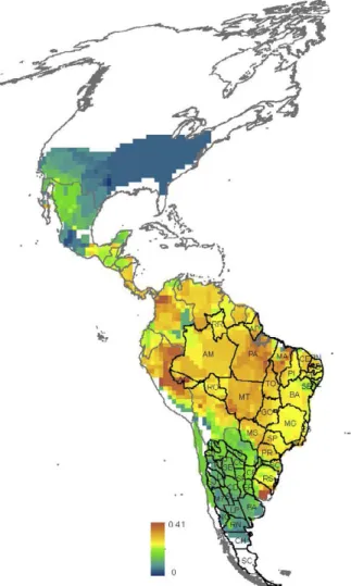
Geographic patterns in Triatominae diversity and Chagas disease - In most Latin American countries, multiple initiatives have been implemented to control Chagas disease vectors based on entomological and epi-demiological criteria (Guhl 2009). In Brazil, the spatial distribution of mean mortality rates caused by Chagas disease per 100,000 inhabitants/year between 1999-2007 shows a clear concentration of municipalities with high mortality in the Central-West Region, including the Fed-eral District, major parts of the state of Goiás and the so-called Triângulo Mineiro region of northwestern of the state of Minas Gerais and north of the state of São Paulo (SP); some areas of the states of Mato Grosso do Sul, Bahia (BA) and Tocantins are also affected and addi-tional small high-mortality areas are found in the border between the state of Paraná and SP, in southern state of
Piauí and in north-central regions of BA (Martins-Melo et al. 2012a). Our study showed that the heterogeneous and focal distribution of those areas of high mortality risk greatly overlapped areas of high SR in Brazil [compare Fig. 2 in Martins-Melo et al. (2012a) with Supplementary data 4, Fig. S5]. This may have important consequences for planning control actions. It has been observed that despite the recent elimination of the most important vector species in Brazil (Triatoma infestans), the spatial clusters of high mortality areas have remained relatively stable over time (Martins-Melo et al. 2012a). In addition, although certain Regions of Brazil (Central-West and Southeast) have seen a steady decline in mortality due to Chagas disease after efforts were concentrated to elimi-nate the primary vector T. infestans, in other regions (North and Northeast), a reduction in mortality rates re-quired interventions to control other prevailing vectors (Martins-Melo et al. 2012b). Vector species of subtropi-cal affinity (i.e., those whose geographisubtropi-cal distributions largely encompass subtropical latitudes of South Ameri-ca: T. infestans, Triatoma brasiliensis, Triatoma sordida and Panstrongylus megistus) tend to show extensive overlap with sites having high triatomine SR (Supple-mentary data 4, Fig. S7A-D). Hence, in the absence of reliable information or underreporting of mortality data, areas of high triatomine SR could be considered pre-liminary indicator areas of high potential mortality risk within the subtropics of South America. In parallel with this reasoning, we suggest that in Argentina, the high-richness area encompassing the eastern portion of the provinces of Jujuy, Salta, Tucuman, Catamarca and La Rioja, the northeastern areas of San Luis province, the northwest part of Cordoba province, the eastern region of Santiago del Estero province and the borders between the provinces of Salta, Chaco and Formosa (Supplemen-tary data 4, Fig. S5) deserve priority in the development of policies involving vector control.
Within the tropics, there are regions of high triatom-ine SR in Venezuela, in Andean regions in Ecuador, Co-lombia and northern Peru and Brazil in the state of Pará close to the Amazon River mouth (Supplementary data 4, Fig. S5). However, there are only two vector species (Triatoma maculate and Panstrongylus geniculatus) of tropical affinity (i.e., those constrained to live within tropical latitudes of South and Central America) associ-ated with high-richness regions (Supplementary data 4, Fig. S7E, L); the remaining vectors of tropical affinity (Rhodnius prolixus, Triatoma dimidiata, Rhodnius pall-escens, Rhodnius ecuatoriensis, Rhodnius robustus and Rhodnius brethesi) tend to overlap sites with low, inter-mediate and high SR in similar proportions (Supplemen-tary data 4, Fig. S7F-K). Thus, we predict that centres of high triatomine SR could be more closely associated with centres of high mortality risk in the subtropics rath-er than in the tropics of South Amrath-erica.
propor-tion of sites of intermediate MDiv (Supplementary data 4, Fig. S8A-D). In contrast, the geographical distribution of vector species of tropical affinity is associated with sites of high MDiv (Supplementary data 4, Fig. S8F-K). In addition, vector species of subtropical affinity are rep-resented in assemblages of species that are more similar or dissimilar than expected by chance (Supplementary data 4, Fig. S9A-D), whereas those of tropical affinity are represented in assemblages that are more dissimi-lar than expected by chance (Supplementary data 4, Fig. S9E-L). Although the possible implications of these patterns remain to be elucidated in terms of the epide-miology of Chagas disease, the present study suggests that analyses of biogeographical patterns in Triatominae diversity may complement analyses of the spatial varia-tion in epidemiological parameters (Martins-Melo et al. 2012a, b) in attempts to define strategies for vector con-trol at a large spatial scale in the Neotropics.
ACKNOWLEDGEMENTS
To JA Diniz-Filho and Juan Morales, for contribution with helpful comments to improve an early version of the paper.
REFERENCES
Addo-Bediakko A, Chown SL, Gaston KJ 2000. Thermal tolerance, climatic variability and latitude. Proc Biol Sci 267: 739-745.
Arita HT, Figueroa F 1999. Geographic patterns of body-mass diver-sity in Mexican mammals. Oikos 85: 310-319.
Bargues MD, Schofield CJ, Dujardin JP 2010. Classification and phy-logeny of the Triatominae. In J Telleria, M Tibayrenc, American trypanosomiasis: Chagas disease one hundred years of research, Elsevier, London, p. 117-148.
Belmaker J, Jetz W 2011. Cross-scale variation in species richness-environment associations. Glob Ecol Biogeogr 20: 464-474.
Borcard D, Legendre P 2002. All-scale spatial analysis of ecological data by means of principal coordinates of neighbour matrices.
Ecol Model 153: 51-68.
Borcard D, Legendre P, Avois-Jacquet C, Tuomisto H 2004. Dissect-ing the spatial structure of ecological data at multiple scales.
Ecology 85: 1826-1832.
Borcard D, Legendre P, Drapeau P 1992. Partialling out the spatial component of ecological variation. Ecology 73: 1045-1055.
Brehm G, Fiedler K 2004. Bergmann’s rule does not apply to geome-trid moths along an elevational gradient in an Andean montane rain forest. Glob Ecol Biogeogr 13: 7-14.
Cabrera A, Willink A 1980. Biogeografía de América Latina. Monografía 13, Secretaría General de la Organización de los Es-tados Americanos/Programa Regional de Desarrollo Científico y Tecnológico, Washington DC, 122 pp.
Calcagno V, Mazancourt C 2010. Glmulti: an R package for easy au-tomated model selection with (generalized) linear models. J Stat Softw 34: 1-29.
Carcavallo RU, Curto de Casa SI, Sherlock IA, Galíndez-Girón I, Jur- berg J, Galvão C, Mena Segura CA, Noireau F 1998a. Geographical distribution and Alti - Latitudinal dispersión. In RU Carcavallo, I Galíndez-Girón, J Jurberg, H Lent, Atlas of Chagas disease vec-tors in the Americas,Fiocruz, Rio de Janeiro, p. 747-792.
Carcavallo RU, da Silva Rocha D, Galíndez Girón I, Sherlock I, Galvão C, Martínez A, Tonn RJ, Cortón E 1998b. Feeding sourc-es and patterns. In RU Carcavallo, I Galíndez-Girón, J Jurberg, H
Lent, Atlas of Chagas disease vectors in the Americas,Fiocruz, Rio de Janeiro, p. 537-560.
Carcavallo RU, Franca Rodríguez ME, Salvatella R, Curto de Casas SI, Sherlock IS, Galvão C, Rocha DS, Galíndez-Girón MA, Ot-ero Arocha MA, Martínez A 1998c. Habitats and related fauna. In RU Carcavallo, I Galíndez-Girón, J Jurberg, H Lent, Atlas of Chagas disease vectors in the Americas,Fiocruz, Rio de Janeiro, p. 561-600.
Carcavallo RU, Jurberg J, Lent H 1999. Phylogeny of the Triatomi-nae. A General approach. In RU Carcavallo, I Galíndez-Girón, J Jurberg, H Lent, Atlas of Chagas disease vectors in the Americas, Fiocruz, Rio de Janeiro, p. 925-969.
Chase JM 2007. Drought mediates the importance of stochastic com-munity assembly. Proc Natl Acad Sci USA 4: 17430-17434.
Chesson P 2000. Mechanisms of maintenance of species diversity.
Annu Rev Ecol Syst 31: 343-366.
Chesson P, Huntly N 1997. The roles of harsh and fluctuating con-ditions in the dynamics of ecological communities. Am Nat 50: 519-553.
Cohen D 2004. The evolutionary ecology of species diversity in stressed and extreme environments. In J Seckbach, Origins. Gen-esis, evolution and diversity of life,Kluwer Academic Publishers, Dordrecht, p. 503-514.
Collar DC, Near TJ, Wainwright PC 2005. Comparative analysis of morphological diversity: does disparity accumulate at the same rate in two lineages of centrarchid fishes? Evolution 59: 1783-1794.
Colwell RK 1974. Predictability, constancy and contingency of peri-odic phenomena. Ecology 55: 1148-1153.
Cumming GS, Child MF 2009. Contrasting spatial patterns of taxo-nomic and functional richness offer insights into potential loss of ecosystem services. Philos Trans R Soc Lond B Biol Sci 364: 1683-1692.
Davies JT, Meiri S, Barraclough TG, Gittleman JL 2007. Species co-existence and character divergence across carnivores. Ecol Lett 10: 146-152.
de Bello F 2012. The quest for trait convergence and divergence in community assembly: are null-models the magic wand? Glob Ecol Biogeogr 21: 312-317.
Devictor V, Mouillot D, Meynard C, Jiguet F, Thuiller W, Mouquet N 2010. Spatial mismatch and congruence between taxonomic, phy-logenetic and functional diversity: the need for integrative conser-vation strategies in a changing world. Ecol Lett 13: 1030-1040.
Diniz-Filho JAF, Bini LM 2005. Modelling geographical patterns in species richness using eigenvector-based spatial filters. Global Ecol Biogeog 14: 177-185.
Diniz-Filho JAF, Bini LM, Hawkins BA 2003. Spatial autocorrelation and red herrings in geographical ecology. Glob Ecol Biogeogr 12: 53-64.
Diniz-Filho JAF, Ceccarelli S, Hasperué W, Rabinovich J 2013. Geo-graphical patterns of Triatominae (Heteroptera: Reduviidae) richness and distribution in the Western Hemisphere. Insect Con-serv Divers doi: 10.1111/icad.12025.
Diniz-Filho JAF, de Marco Jr P, Hawkins BA 2010. Defying the curse of ignorance: perspectives in insect macroecology and conserva-tion biogeography. Insect Conserv Divers 3: 172-179.
Diniz-Filho JAF, Rangel TFLVB, Bini LM 2008. Model selection and information theory in geographical ecology. Glob Ecol Biogeogr 17: 479-488.
Meth-ods to account for spatial autocorrelation in the analysis of spe-cies distributional data: a review. Ecography 30: 609-628.
ESRI 2007. ArcGIS™ [GIS Software], v. 9.2, Environmental Systems Research Institute, Inc, Redlands, CA, USA.
Field R, Hawkins BA, Cornell HV, Currie DJ, Diniz-Filho JAF, Guégan JF, Kaufman DM, Kerr JT, Mittelbach GG, Oberdorff T 2009. Spatial species richness gradients across scales: a meta analysis. J Biogeogr 36: 132-147.
Foote M 1993. Discordance and concordance between morphological and taxonomic diversity. Paleobiology 19: 185-204.
Galíndez-Girón I, Carcavallo RU, Jurberg J, Galvão C, Lent H, Barata JMS, Pinto Serra O, Valderrama A 1998. Morfology and external anatomy. In RU Carcavallo, I Galíndez-Girón, J Jurberg, H Lent,
Atlas of Chagas disease vectors in the Americas,Fiocruz, Rio de Janeiro, p. 53-73.
Gatz Jr AJ 1979. Community organization in fishes as indicated by morphological features. Ecology 60: 711-718.
Gilbert FS 1985. Ecomorphological relationships in hoverflies (Dip-tera, Syrphidae). Proc Biol Sci 224: 91-105.
Gomez JP, Bravo GA, Brumfield RT, Tello JG, Cadena CD 2010. A phylogenetic approach to disentangling the role of competition and habitat filtering in community assembly of Neotropical forest birds. J Anim Ecol 79: 1181-1192.
Gommes R, Grieser J, Bernardi M 2004. FAO agroclimatic databases and mapping tools. Eur Soc AgronNewsl 22: 32-36.
Gould SJ, Lewontin RC 1979. The spandrels of San Marco and the Panglossian paradigm: a critique of the adaptationist programme.
Proc Biol Sci 205: 581-598.
Gower JC 1971. A general coefficient of similarity and some of its properties. Biometrics27: 857-871.
Guhl F 2009. Enfermedad de Chagas: realidad y perspectivas. Rev Biomed 20: 228-234.
Harvey PH, Pagel MD 1991. The comparative method in evolutionary biology, Oxford University Press, Oxford, 248 pp.
Hawkins BA, Field R, Cornell HV, Currie DJ, Guégan JF, Kaufman DM, Kerr JT, Mittelbach GG, Berdorff TC, O’Brien EM, Porter EE, Turner JRG 2003. Energy, water and broad-scale geographic patterns of species richness. Ecology84: 3105-3117.
Hawkins BA 2012. Eight (and a half) deadly sins of spatial analysis.
J Biogeogr 39: 1-9.
Hay SI, Tatem AJ, Graham AJ, Goetz SJ, Rogers DJ 2006. Global environmental data for mapping infectious disease distribution.
Adv Parasitol 62: 37-77.
Hijmans RJ, Cameron SE, Parra JL, Jones PG, Jarvis A 2005. Very high resolution interpolated climate surfaces for global land ar-eas. Int J Climatol25: 1965-1978.
Hubbell SP 2001. The unified neutral theory of biodiversity and bio-geography. Monographs in Population Biology 32, Princeton University Press, Princenton and Oxford, 375 pp.
Hypsa V, Tietz DF, Zrzavy J, Rego ROM, Galvão C, Jurberg J 2002. Phylogeny and biogeography of Triatominae (Hemiptera: Redu-viidae): molecular evidence of a New World origin of the Asiatic clade. Mol Phylogenet Evol 23: 447-457.
Keddy PA 1992. Assembly and response rules: two goals for predic-tive community ecology. J Veg Sci 3: 157-164.
Kubota U, Loyola RD, Almeida AM, Carvalho DA, Lewinsohn TM 2007. Body size and host range co-determine the altitudinal dis-tribution of Neotropical tephritid flies. Glob Ecol Biogeogr16: 632-639.
Laliberté E, Legendre P 2010. A distance-based framework for measur-ing functional diversity from multiple traits. Ecology91: 299-305.
Leibold MA 1998. Similarity and local co-existence of species in re-gional biotas. Evol Ecol12: 95-110.
Lent H, Carcavallo RU, Martínez A, Galíndez-Girón I, Jurberg J, Galvão C, Canale DM 1998. Anatomic relationships and charac-terization of the species. In RU Carcavallo, I Galíndez-Girón, J Jurberg, H Lent, Atlas of Chagas disease vectors in the Americas, Fiocruz, Rio de Janeiro, p. 53-73.
Lent H, Wygodzinsky P 1979. Revision of the Triatominae (Hemiptera, Reduviidae) and their significance as vectors of Chagas disease.
Bull Amer Mus Nat Hist 163: 123-520.
MacArthur R, Levin R 1964. Competition, habitat selection and char-acter displacement in a patchy environment. Proc Natl Acad Sci USA 51: 1207-1210.
Martins-Melo FR, Ramos AN, Alencar CH, Lange W, Heukelbach J 2012a. Mortality of Chagas disease in Brazil: spatial patterns and definition of high-risk areas. Trop Med Int Health 17: 1066-1075.
Martins-Melo FR, Ramos Jr AN, Alencar CH, Lange W, Heukelbach J 2012b. Mortality due to Chagas disease in Brazil from 1979 to 2009: trends and regional differences. J Infect Dev Ctries 6: 817-824.
Medone P, Rabinovich JE, Nieves E, Ceccarelli S, Canale D, Stariolo RL, Menu F 2012. The Quest for immortality in Triatomines: a meta-analysis of the senescence process in hemimetabolous he-matophagous insects. In T Nagata (eds.), Senescence, INTECH, Rijeka, p. 225-250.
Meynard CN, Devictor V, Mouillot D, Thuiller W, Jiguet F, Mouquet
N 2011. Beyond taxonomic diversity patterns: how do α, β and γ components of bird functional and phylogenetic diversity re -spond to environmental gradients across France? Glob Ecol Bio-geogr20: 893-903.
Neustupa J, Černá K, Št’astný J 2009. Diversity and morphological
disparity of desmid assemblages in Central European peatlands.
Hydrobiologia630: 243-256.
New M, Hulme M, Jones P 1999. Representing twentieth-century space-time climate variability. Part I. Development of a 1961-90 mean monthly terrestrial climatology. J Clim12: 829-857.
Olson DM, Dinerstein E, Wikramanayake ED, Burgess ND, Powell GVN, Underwood EC, D’Amico JA, Itoua I, Strand HE, Mor-rison JC 2001. Terrestrial ecoregions of the world: a new map of life on earth. BioScience51: 933-938.
Patterson BD, Willig MR, Stevens RD 2003. Trophic strategies, niche partitioning and patterns of ecological organization. In TH Kunz, MB Fenton, Bat ecology,University of Chicago Press, Chicago, p. 536-579.
Patterson JS, Guhl F 2010. Geographical distribution of Chagas disease. In J Telleria, M Tibayrent, American trypanosomiasis: Chagas dis-ease one hundred years of research, Elsevier, London, p. 83-114.
Pereira MH, Gontijo NF, Guarneri AA, Sant’Anna MR, Diotaiuti L 2006. Competitive displacement in Triatominae: the Triatoma in-festans success. Trends Parasitol 22: 516-520.
Petchey OL, Evans KL, Fishburn IS, Gaston KJ 2007. Low functional diversity and no redundancy in British avian assemblages. J Anim Ecol76: 977-985.
Podani J 2009. Convex hulls, habitat filtering and functional diver-sity: mathematical elegance versus ecological interpretability.
Community Ecol10: 244-250.
Rabinovich JE, Kitron UD, Obed Y, Yoshioka M, Gottdenker N, Chaves LF 2011. Ecological patterns of blood-feeding by kissing-bugs (Hemiptera: Reduviidae: Triatominae). Mem Inst Oswaldo Cruz 106: 479-494.
Rangel TF, Diniz-Filho JAF, Bini LM 2010. SAM: a comprehensive application for spatial analysis in macroecology. Ecography33: 46-50.
Rodriguero MS, Gorla DE 2004. Latitudinal gradient in species rich-ness of the New World Triatominae (Reduviidae). Glob Ecol Bio-geogr13: 75-84.
Rodríguez J, Hortal J, Nieto M 2006. An evaluation of the influence of environment and biogeography on community structure: the case of Holarctic mammals. J Biogeogr33: 291-303.
Roig FA, Roig-Juñent S, Corbalán V 2009. Biogeography of the Mon-te desert. J Arid Environ73: 164-172.
Roy K, Balch DP, Hellberg ME 2001. Spatial patterns of morpho-logical diversity across the Indo-Pacific: analyses using strombid gastropods. Proc Biol Sci 268: 2503-2508.
Roy K, Foote M 1997. Morphological approaches to measuring biodi-versity. Trends Ecol Evol12: 277-281.
Rundle SD, Bilton DT, Abbott JC, Foggo A 2007. Range size in North American Enallagma damselflies correlates with wing size.
Freshw Biol52: 471-477.
Safi K, Cianciaruso MV, Loyola RD, Brito D, Armour-Marshall K, Diniz-Filho JAF 2011. Understanding global patterns of mam-malian functional and phylogenetic diversity. Philos Trans R Soc Lond B Biol Sci 366: 2536-2544.
Schachter-Broide J, Dujardin J-P, Kitron U, Gürtler RE 2004. Spa-tial structuring of Triatoma infestans (Hemiptera, Reduviidae) populations from northwestern Argentina using wing geometric morphometry. J Med Entomol41: 643.
Schluter D 2000. The ecology of adaptive radiation, Oxford Univer-sity Press, New York, 296 pp.
Schofield CJ, Galvão C 2009. Classification, evolution and species groups within the Triatominae. Acta Trop110: 88-100.
Shepherd UL 1998. A comparison of species diversity and morpho-logical diversity across the North American latitudinal gradient.
J Biogeogr25: 19-29.
Shepherd UL, Kelt DA 1999. Mammalian species richness and mor-phological complexity along an elevational gradient in the arid south west. J Biogeogr26: 843-855.
Silva de Paula A, Diotaiuti L, Schofield CJ 2005. Testing the sister-group relationship of the Rhodniini and Triatomini (Insecta: Hemiptera: Reduviidae: Triatominae). Mol Phylogenet Evol 35: 712-718.
Siqueira T, de Oliveira Roque F, Trivinho-Strixino S 2008. Species richness, abundance and body size relationships from a Neotropi-cal chironomid assemblage: looking for patterns. Basic Appl Ecol 9: 606-612.
Stevens RD, Willig MR, Strauss RE 2006. Latitudinal gradients in the phenetic diversity of New World bat communities. Oikos112: 41-50.
Turchetto-Zolet AC, Pinheiro F, Salgueiro F, Palma-Silva C 2013. Phylogeographical patterns shed light on evolutionary process in South America. Mol Ecol22: 1193-1213.
Venner S, Pélisson P-F, Bel-Venner M-C, Débias F, Rajon E, Menu F 2011. Coexistence of insect species competing for a pulsed resource: toward a unified theory of biodiversity in fluctuating environments. PloS ONE6: e18039.
TABLE SI List of the 91 species studied
Alberprosenia goyovargasi Triatoma circummaculata
Belminus costaricensis Triatoma costalimai
Belminus herreri Triatoma delpontei
Belminus laportei Triatoma dimidiata
Belminus peruvianus Triatoma dispar
Bolbodera scabrosa Triatoma eratyrusiforme
Cavernicola pilosa Triatoma flavida
Dipetalogaster maximus Triatoma garciabesi
Eratyrus cuspidatus Triatoma gerstaeckeri
Eratyrus mucronatus Triatoma guasayana
Mepraia spinolai Triatoma guazu
Microtriatoma borbai Triatoma incrassata
Microtriatoma trinidadensis Triatoma indictiva
Panstrongylus geniculatus Triatoma infestans
Panstrongylus guentheri Triatoma lecticularia
Panstrongylus howardi Triatoma lenti
Panstrongylus lignarus Triatoma limai
Panstrongylus lutzi Triatoma longipennis
Panstrongylus megistus Triatoma maculata
Panstrongylus rufotuberculatus Triatoma matogrossensis
Panstrongylus tupynambai Triatoma mazzotti
Parabelminus carioca Triatoma melanocephala
Parabelminus yurupucu Triatoma melanosoma
Paratriatoma hirsuta Triatoma neotomae
Psammolestes arthuri Triatoma nigromaculata
Psammolestes coreodes Triatoma nitida
Psammolestes tertius Triatoma oliveirai
Rhodnius brethesi Triatoma pallidipennis
Rhodnius dalessandroi Triatoma patagonica
Rhodnius domesticus Triatoma peninsularis
Rhodnius ecuadoriensis Triatoma petrochii
Rhodnius nasutus Triatoma phyllosoma
Rhodnius neglectus Triatoma picturata
Rhodnius neivai Triatoma platensis
Rhodnius pallescens Triatoma protracta
Rhodnius paraensis Triatoma pseudomaculata
Rhodnius pictipes Triatoma recurva
Rhodnius prolixus Triatoma rubida
Rhodnius robustus Triatoma rubrovaria
Rhodnius stali Triatoma ryckmani
Triatoma arthurneivai Triatoma sanguisuga
Triatoma brasiliensis Triatoma sinaloensis
Triatoma breyeri Triatoma sordida
Triatoma bruneri Triatoma tibiamaculata
Triatoma carcavalloi Triatoma vitticeps
a: evaluation of the effect of spatial autocorrelation on the performance of environmental models fitted to morphological
diversity (MDiv) and species richness (SR) - We checked the adequacy of the environmental models shown on Tables I (main text)
to account for the geographic variation in MDiv and SR in the presence of spatial autocorrelation.
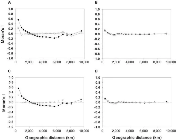
We elaborated spatial correlograms using Moran’s I coefficient to describe the magnitude of autocorrelation of MDiv and SR for different distance classes. Then, we examined the spatial patterns of autocorrelation in their residuals after the fit of the models shown on Table I. Independently of the pattern of autocorrelation in the original (predictors and response) variables, if no spatial autocorrelation is found in the residuals it can be concluded that the model had taken into account all spatial structure in the original data and that there was no statistical bias in the overall statistical analysis (Diniz-Filho et al. 2003).
The spatial correlogram for MDiv (Fig. S2A) showed a quadratic pattern that indicated the presence of positive autocorrela-tion up to c.3100 km, then the negative autocorrelaautocorrela-tion increased strongly to reach -0.8 at c.6200 km and then it progressively decreased to approach low values (i.e. between 0-0.2) at the largest distance classes. SR showed high positively autocorrelation (0.61) at the shortest distance class (c.400km), then the autocorrelation decreased up to c.4,000 km and then it increased again to reach -0.49 at c.7,500 km (Fig. S2B).
After model fit, the autocorrelation in the residuals of MDiv at the shortest distance classes (c.400 km) (Fig. S2A) decreases from 0.80-0.30 and decreases to < 0.1 for all subsequent distance classes up to c.7,400 km; the spatial autocorrelation increases again at distance classes > 8,000 km, although coefficients are never larger than 0.2 (Fig. S2A). Similarly, the autocorrelation in the residuals of SR decreases from 0.61-0.38 at the shortest distance classes and then remained between 0-0.15 for all subsequent distance classes (Fig. S2B).
b: the modeling of the spatial patterns of autocorrelation of MDiv and SR - We modeled the spatial structure of MDiv and SR
by the spatial eigenvector mapping (SEVM) routine in SAM v4 (Rangel et al. 2010). We conducted separate SVEM analyses for MDiv and SR. The SEVM uses the spatial coordinates of the grid cells to construct a spatial matrix from which to extract eigen-vectors that allow the decomposition of the whole spatial structure in the data into spatial patterns at different spatial scales [see Borcard and Legendre (2002) for a formal description of method] (Diniz-Filho & Bini 2005, Rangel et al. 2010). In this way, the neighborhood relationships among the grid cells were used to reveal the spatial autocorrelation of our data set over the whole range of scales encompassed by the sampling design (Borcard & Legendre 2002, Borcard et al. 2004, Diniz-Filho & Bini 2005).
We detrended the data on SR from a significant linear longitudinal trend fitted by least squares and data on MDiv from two significant (linear and quadratic) latitudinal trends so that the method would be able to recover finer spatial structures (Borcard & Legendre 2002, Borcard et al. 2004). We adopted the criterion of minimisation of Moran’s I in model residuals available in SAM v.4 to select those eigenvectors that were the best spatial descriptors of the spatial patterns of autocorrelation for MDiv and SR (Rangel et al. 2010).
SAM v.4 selected 61 positive eigenvectors as spatial descriptors of the latitudinally detrended MDiv and 63 were selected to model the spatial variation in longitudinally detrended SR (eigenvectors not shown) that reduced the spatial structure in MDiv and SR at all spatial scales to almost zero (Fig. S3A, B). The spatial descriptors of SR and MDiv were poorly correlated with the environmental variables retained in models shown on Table I; for SR, the correlation coefficients (r) ranged from r = -0.32-0.31 and for MDiv, from -0.38-0.28. Hence, the spatial descriptors provided complementary information about the spatial structure of MDiv and SR not fully accounted by the environmental variables.
c: partial regression analysis to partition the variation in MDiv and SR - We combined the spatial descriptors obtained from
SEVM with the environmental predictors shown in Table I (main text) in a partial regression analysis. Given that the environ-mental predictors and spatial descriptors were poorly correlated (see above), the combination of them in statistical models did not introduce a serious problem of multicollinearity (Hawkins 2012).
As explained in Borcard et al. (1992), we partitioned the variation in MDiv and SR into: (a) the fraction of MDiv and SR explained by environmental descriptors independently of any spatial structure; (b) the fraction of the variation in MDiv and SR explained by the shared variation between spatial descriptors and environmental variables; (c) the spatial variation in MDiv or SR not shared by the environmental variables analysed, which suggests the operation of some underlying biological process that has no apparent relation to the environmental variables that were included in our analysis and (d) the fraction of the MDiv and SR variation explained neither by the spatial coordinates nor by environmental data. All calculations were done for MDiv and SR separately and based on:
The R2 of the regression model that combined the environmental descriptors in Table I (main text) that provided information
of fractions (a) and (b) above (R2 = a + b).
The R2 of the regression model that combined the spatial descriptors obtained from SVEM and that provided information about
fractions (c) and (b) above (R² = c + b). The spatial descriptors of MDiv were the linear and quadratic terms of latitude and 61 posi-tive eigenvectors selected by the SVEM routine; for SR, the spatial descriptors were longitude and 63 posiposi-tive eigenvectors.
The R2 of the regression model that combined the whole set of environmental and spatial descriptors (full regression model)
that provided information about fractions (a), (b) and (c) above (R² = a + b + c).
According to Borcard et al. (1992), each component of variation was computed from simple calculations: b = (a + b) + (b + c) - (a + b + c),
Fig. S2: spatial correlograms for (A) morphological diversity and (B) species richness (SR) (solid circles) and residuals (open circles) of morpho-logical diversity (A) and SR (B) after fitting the environmental models shown on Table I (main text). AIC: Akaike’s information criterion.