CLIMATE CHANGES AND THEIR EFFECTS IN THE PUBLIC HEALTH: USE OF POISSON REGRESSION MODELS
Jonas Bodini Alonso
Departamento de Estatística / IMECC
Universidade Estadual de Campinas (UNICAMP) Campinas – SP, Brasil
Jorge Alberto Achcar
Departamento de Medicina Social / FMRP Universidade de São Paulo (USP) Ribeirão Preto – SP, Brasil
Luiz Koodi Hotta*
Departamento de Estatística / IMECC
Universidade Estadual de Campinas (UNICAMP) Campinas – SP, Brasil
* Corresponding author / autor para quem as correspondências devem ser encaminhadas
Recebido em 12/2008; aceito em 09/2009
Received December 2008; accepted September 2009
Abstract
In this paper, we analyze the daily number of hospitalizations in São Paulo City, Brazil, in the period of January 01, 2002 to December 31, 2005. This data set relates to pneumonia, coronary ischemic diseases, diabetes and chronic diseases in different age categories. In order to verify the effect of climate changes the following covariates are considered: atmosphere pressure, air humidity, temperature, year season and also a covariate related to the week day when the hospitalization occurred. The possible effects of the assumed covariates in the number of hospitalization are studied using a Poisson regression model in the presence or not of a random effect which captures the possible correlation among the hospitalization accounting for the different age categories in the same day and the extra-Poisson variability for the longitudinal data. The inferences of interest are obtained using the Bayesian paradigm and MCMC (Markov chain Monte Carlo) methods.
Keywords: daily hospitalizations; climate changes; Bayesian analysis; MCMC methods.
Resumo
Neste artigo, analisamos os dados relativos aos números diários de hospitalizações na cidade de São Paulo, Brasil no período de 01/01/2002 a 31/12/2005 devido a pneumonia, doenças isquêmicas, diabetes e doenças crônicas e de acordo com a faixa etária. Com o objetivo de estudar o efeito de mudanças climáticas são consideradas algumas covariáveis climáticas os índices diários de pressão atmosférica, umidade do ar, temperatura e estação do ano, e uma covariável relacionada ao dia da semana da ocorrência de hospitalização. Para verificar os efeitos das covariáveis nas respostas dadas pelo numero de hospitalizações, consideramos um modelo de regressão de Poisson na presença ou não de um efeito aleatório que captura a possível correlação entre as contagens para as faixas etárias de um mesmo dia e a variabilidade extra-poisson para os dados longitudinais. As inferências de interesse são obtidas usando o paradigma bayesiano e métodos de simulação MCMC (Monte Carlo em Cadeias de Markov).
1. Introduction
An important problem related to public health is the possible relationship between climate factor levels and the incidence of some specific diseases. Great climate variations have been observed in the last years due to many different factors, in special, the degradation of the environmental conditions linked to the fast population increasing. In this way, there is a great interest by doctors of the public health to study the existing relations between the daily hospitalization countings due to some specific diseases with some daily climate levels as atmospheric pressure, air humidity and temperature. The effects of climate variations can be larger in high-risk age groups as newborns or old age persons. One way of considering this situation is the use of counting regression model for each age group. A special model for counting data is given by a Poisson regression model capturing the possible existing correlation among the hospitalization daily counting in each age class. Longitudinal Poisson data is common in many applications considering medical studies (see for example, Henderson & Shikamura, 2003; or Dunson & Herring, 2005), where the counting are measures for each sampling unit in different times or repeated measures.
In this study, we consider a data set related to the daily hospitalization counting due to pneumonia, coronary ischemic diseases, diabetes and chronic diseases in different age categories in the São Paulo city in the period ranging from 01/01/2002 to 12/31/2005 and classified in different patient age groups and in the presence of some climate covariates.
The hospitalization group denoted as Pneumonia is related to the codes J10 to J18 of the CID 10; the hospitalization group denoted as Chronic Diseases (of upper airways) is related to the codes J40 to J47 of the CID 10; the hospitalization group denoted as Coronary Ischemic Diseases is related to the codes I20 to I25 of the CID 10 and the hospitalization group denoted as Diabetes (Mellitus) is related to the codes E10 to E14 of the CID 10. This codification is used by the health system SUS of the São Paulo city and were available by the health office of the São Paulo city.
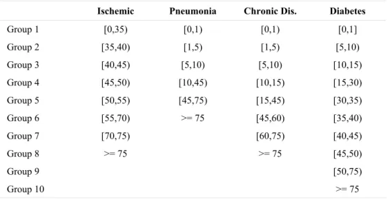
The age categories are defined taking as basis the group classification used by the Department of informatics of the Brazilian health system (DATASUS). In this system a person is classified as group 0 for ages up to 1 year old; group 1 for ages from 1 year old to 5 years old; group 2 for ages from 5 years old to 10 years old; and so on up to group 16 that includes persons aging more than 75 years old. In our study, we consider some special aggregation of these groups depending on the type of hospitalization. Two age neighboring groups for one type of hospitalization are aggregated in the same age group if they have similar behavior in term of number of hospitalization. The group classifications for each type of hospitalization are presented in table 1.
The climate data were available from the Institute of Astronomy and Geophysics of the University of São Paulo (IAG-USP). The climate covariates considered in this study are the daily average of atmospheric pressure, the daily average of air humidity and the daily average of temperature. These average levels are found considering the average of the daily observed maximum and minimum in each day. We also considered other covariates, as year seasons and weekly days.
Table 1 – Age groups based on an exploratory data analysis. Age in complete years. Ischemic Pneumonia Chronic Dis. Diabetes
Group 1 [0,35) [0,1) [0,1) [0,1]
Group 2 [35,40) [1,5) [1,5) [5,10)
Group 3 [40,45) [5,10) [5,10) [10,15)
Group 4 [45,50) [10,45) [10,15) [15,30)
Group 5 [50,55) [45,75) [15,45) [30,35)
Group 6 [55,70) >= 75 [45,60) [35,40)
Group 7 [70,75) [60,75) [40,45)
Group 8 >= 75 >= 75 [45,50)
Group 9 [50,75)
Group 10 >= 75
To analyze this data set, we introduce two Poisson regression models in the presence or absence of a random factor which captures the correlation between the repeated measures for the same day and the presence of extra-Poisson variability for the data (see, for example, Albert, 1992; Achcar et al., 2008).
Poisson regression models in the presence of frailties or random effects have been considered by many authors (see, for example, Crouchley & Davies, 1999; Korsgaard & Andersen, 1998; Legler & Ryan, 1997; Li, 2002; Moustaki & Knott, 2000; Petersen, 1998; or Sammel et al., 1997).
The inferences of interest are obtained using Bayesian methods. The posterior summaries of interest are obtained via MCMC simulation methods as the popular Gibbs sampling algorithm (see, for example, Gelfand & Smith, 1990) or the Metropolis-Hastings algorithm (see, for example, Chib & Greenberg, 1995).
The paper is organized as follows. In section 2, we introduce the statistical model. Section 3 introduces a Bayesian analysis for the models. Section 4 introduces the analysis of the São Paulo City data set. Finally, Section 5 presents a discussion about the obtained results.
2. The Statistical Model
Let Nij a random variable with Poisson distribution, i.e.
(
ij ij)
exp( )
ij ij( )
nij / ijP N = n = −λ λ n !, (1)
we consider the presence of covariates x1i (average atmospheric pressure between the minimum and maximum on the i-th day), x2i (average humidity between the minimum and maximum on the i-th day), x3i (average temperature between minimum and maximum on the i-th day) and dummy variables or indicator x4i (equals 1 if the fall in the i-th day, 0 otherwise), x5i (equal to 1 if the winter i-th day, 0 otherwise), x6i (equal to 1 if spring in the i-th day, 0 otherwise), and x7i (equal to 1 if the i-th day is Saturday or Sunday, 0 otherwise).
As we have longitudinal data representing the number of hospitalization on the same day for different age groups, we introduce a random effect or frailty wi that captures the correlation between repeated measurements for the i-th day and extra-Poisson variability.
Assuming a Poisson distribution (1) for Nij with parameter λij , consider the regression model,
( )
exp ij ij i
λ = w , (2)
where
(
)
( )
3 7
1 4
exp
ij j lj li l lj li
l= l=
= ⎛⎜α + β x −x ⎞⎟+ β x
⎝
∑
⎠∑
(3)1 n l li
i=
nx =
∑
x , l = 1,...,3; j=(
αj,β1j,β2j,β3j,β4j,β5j,β6j,β7j)
T , j = 1,...,K is the vector ofunknown parameters and wi is a random effect with normal distribution,
( )
20, i.i.d
~ i
w N σ , (4)
where i = 1, ..., N.
Note that, according to equation (1), since Nij has a Poisson distribution, then,
( )
ij( )
ij ijE N = Var N =λ , where λij is given in (3). Also note that non-conditional means and variances are given by
(
ij/ j i)
(
ij/ j i i)
E N , x = E E N⎡⎣ , x ,w ⎤⎦
and (5)
(
ij/ j j)
(
(
ij/ j i i)
)
(
(
ij/ j i i)
)
Var N , x = Var E N , x ,w + E Var N , x ,w ,
where j is defined in (2) and
(
1i 7i)
T ix = x ,", x is the covariate vector associated with the i-th day.
As the random effects wi have a normal distribution (4), then exp
( )
wi have a log-normaldistribution with mean equals to exp
(
σ2/ 2)
and variance equals to(
2)
(
(
2)
)
(
)
(
2)
/ exp / 2
ij j i ij
E N , x = σ (6)
and
(
)
2(
2)
(
(
2)
)
(
2)
/ exp / 2 exp / 2 1 exp / 2
ij j i i ij ij
Var N , x ,w = σ σ − + σ . (7)
From (6) and (7), we observe that the mean and variance of Nij are different, that is, we
have the presence of an extra-Poisson variability given by ij2exp
(
σ2/ 2 exp)
(
(
σ2/ 2)
−1)
, where ij is given by (3).For the analysis of data from hospitalizations, let us consider two possible models: a model denoted as “Model 1” without the presence of random effect wi and a “Model 2” with the presence of random effects, wi, i = 1,..., N.
Note that the presence of a random effect in the Poisson regression model can hinder the achievement of classical inferences for the parameters of the model. A possible simplification to obtain the inferences of interest is to consider Bayesian methods. In addition, the Bayesian methods allow the incorporation of information from experts in the prior distribution for the model parameters. This methodology has been considered by many authors in the analysis of longitudinal count data (see e.g., Albert & Chib, 1993; Chib et al., 1998; Clayton, 1991; Dunson, 2000, 2003).
3. Bayesian Analysis
Assuming the model given by (2) and (3), the likelihood function for
(
1...)
T k= , , , given the observed data Nij , the unobserved variables wi and the vector of covariates xij , is given by
( )
( )
( )
1 1
exp /
N K
nij ij ij ij i= j=
L =
∏∏
−λ λ n !. (8)For the first stage of the hierarchical Bayesian analysis, assuming “Model 2” in the presence of random effects wi, we consider the following prior distributions for model parameters
(
2)
j j j
α ~ N a ,b , βlj ~ N
( )
0,c2j , (9)where l = 1, ..., 7 ; j = 1,...,K ; aj, bj and cj are known hyperparameters.
For the second stage of the hierarchical Bayesian analysis, where wi has a normal
distribution N
(
0,σ2)
, we assume that( )
2where d and e are known parameters, and Gamma (d, e) denotes a gamma distribution with mean d e/ and variance d e/ 2. We assume that the prior distributions of the parameters are independent.
For “Model 1” without the presence of random effect wi, we assume the same prior distributions for αj and βlj given in (9).
The joint posterior distribution for and σ2 is obtained by combining the likelihood function (8) with the prior joint distribution for the parameters and wi, i.e.
(
)
( )
(
)
(
(
)
)
(
)( )
( )(
)
2
2 2 2 2
1
7 1
2 2 2 2
1 1
/ exp / 2 exp / 2b
exp / 2c exp
k
i j j j
j=
k d
lj j j= l=
π ,σ N, L w σ α a
β σ − eσ ,
⎡ ⎤
∝ ⎣ − ⎦ − −
− −
∏
∏∏
x(11)
where N is the vector of data Nij , and x is the vector of covariates xli ; the likelihood
function L
( )
is given in (8).Summaries of the a posteriori distributions of interest are obtained using MCMC methods. In this way, we simulate samples from the conditional distributions for each parameter given the other parameters and the vectors of data and covariates.
A great simplification is obtained using the software WinBUGS (Spiegelhalter et al., 2003) that only requires the specification of the distribution to the data and prior distributions for the parameters.
The selection of the best model can be done using several Bayesian discrimination methods available in the literature. In our case we consider the Deviance Information Criterion (DIC) (see Spiegelhalter et al., 2002) which is a useful criterion for selecting models when samples of posterior distribution for the model parameters are obtained using MCMC methods.
The deviance is defined by
( )
2logL( )
D =− + c, (12)
where is a vector of unknown parameters of the model L
( )
is the likelihood function and c is a constant that need not be known in the comparison of models.The DIC criterion is defined by
( )
2nDDIC = D + , (13)
where D
( )
is the deviation of the average evaluated in the posteriori mean and nD is4. Data Analysis of Daily Hospital Admissions in São Paulo City
Initially, let us consider the count data for daily hospital admissions in São Paulo for chronic conditions in the period 01/01/2002 to 31/12/2005. Assuming k = 8 age groups and the “Model 1” without the presence of a random effect with prior distributions given in (9) for αj and βlj ; l = 1, ..., 7; j = 1, ..., 8 and, l = 1, ..., 7, j = 1, ..., 8 and values of the hyperparameters equal to a =j 0,
2
000.1 j
b = and c =2j 1, we have used the WinBUGS software to simulate 1000 samples of the joint posterior distribution for the parameters. After a burn-in-sample of size of 5000, we took samples spaced by 10 in the Gibbs sampling algorithm in order to eliminate the effect of the initial values of parameters used in the iterative procedure and to have approximately uncorrelated samples.
Similarly, with the same steps used to generate samples assuming “Model 1”, we generate 1,000 samples from the joint posterior distribution (10) considering “Model 2” in the presence of random effect wi with normal distribution (4), with d = e = 1 in the prior for σ2 (10) and assuming an informative priori for αj with a =j 1 and b =2j 100. This choice of values of the hyperparameters for the prior was based on the results of “Model 1” to ensure the convergence of the algorithm simulation. For the parameter βlj we used the same values considered for the hyperparameters of “Model 1”.
The convergence of the algorithm was verified from the graphs of the simulated samples.
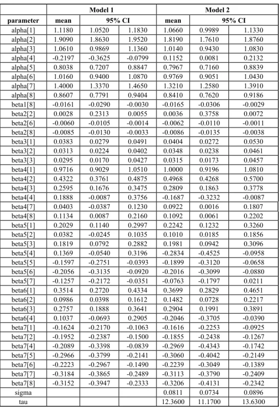
Table 2 presents the summaries of the posterior distributions of interest in case of hospitalization due to chronic diseases for models 1 and 2. The 95% credibility interval is given by 2.5% and 97.5% percentiles of the posteriori distributions. For brevity we present only the results of parameters whose credibility interval of at least one of the models does not include the value zero. The same criteria is used for other type of admissions.
For the choice between the two proposed models, we obtain from the 1000 simulated Gibbs samples, DIC equal to 46,664.9 for “Model 1” and DIC equal to 45,624.5 DIC for “Model 2”. Thus, “Model 2” presents the best adjustment for the data according to DIC criterion because the value of DIC is lower for “Model 2” than for “Model 1”.
We also compare the two models, evaluating the sum of squares of differences, s2
( )
v , v = 1, 2 (models 1 and 2), between the observed counts and means of the Monte Carlo posteriori distribution of λij. For “Model 1” we find( )
2
1 5,3281.3
s = and for “Model 2”, we find
( )
2
1 3,9277.8
s = , which gives strong indication in favor of “Model 2”.
Table 2 – Results for Chronic Diseases.
Model 1 Model 2
parameter mean 95% CI mean 95% CI
alpha[1] 1.1180 1.0520 1.1830 1.0660 0.9989 1.1330
alpha[2] 1.9090 1.8630 1.9520 1.8190 1.7610 1.8760
alpha[3] 1.0610 0.9869 1.1360 1.0140 0.9430 1.0830
alpha[4] -0.2197 -0.3625 -0.0799 0.1152 0.0081 0.2132
alpha[5] 0.8038 0.7207 0.8847 0.7967 0.7160 0.8839
alpha[6] 1.0160 0.9400 1.0870 0.9769 0.9051 1.0430
alpha[7] 1.4000 1.3370 1.4650 1.3210 1.2580 1.3910
alpha[8] 0.8607 0.7791 0.9404 0.8410 0.7620 0.9186
beta1[8] -0.0161 -0.0290 -0.0030 -0.0165 -0.0306 -0.0029
beta2[2] 0.0028 0.2313 0.0055 0.0036 0.3758 0.0072
beta2[6] -0.0060 -0.0105 -0.0014 -0.0062 -0.0110 -0.0011 beta2[8] -0.0085 -0.0130 -0.0033 -0.0086 -0.0135 -0.0038
beta3[1] 0.0383 0.0279 0.0491 0.0404 0.0272 0.0530
beta3[2] 0.0313 0.0224 0.0402 0.0348 0.0238 0.0461
beta3[3] 0.0295 0.0170 0.0427 0.0315 0.0173 0.0457
beta4[1] 0.9716 0.9029 1.0510 1.0000 0.9196 1.0810
beta4[2] 0.4322 0.3761 0.4875 0.4968 0.4268 0.5700
beta4[3] 0.2595 0.1676 0.3475 0.2809 0.1863 0.3778
beta4[4] 0.1888 -0.0087 0.3756 -0.1687 -0.3232 -0.0087 beta4[7] 0.0403 -0.0387 0.1230 0.0922 0.0016 0.1807
beta4[8] 0.1134 0.0087 0.2160 0.1092 0.0061 0.2202
beta5[1] 0.2029 0.1140 0.2997 0.2242 0.1232 0.3260
beta5[2] 0.0382 -0.0245 0.1035 0.1010 0.0185 0.1856
beta5[3] 0.1819 0.0792 0.2882 0.1981 0.0942 0.3096
beta5[4] 0.1369 -0.0540 0.3196 -0.2834 -0.4525 -0.0958 beta5[5] -0.1597 -0.2751 -0.0393 -0.1899 -0.3120 -0.0658 beta5[6] -0.2056 -0.3135 -0.0920 -0.2016 -0.3099 -0.0880 beta5[7] -0.1257 -0.2172 -0.0351 -0.0763 -0.1797 0.0211
beta6[1] 0.3514 0.2720 0.4334 0.3699 0.2829 0.4651
beta6[2] 0.0986 0.0398 0.1612 0.1482 0.0728 0.2217
beta6[3] 0.2757 0.1888 0.3641 0.2904 0.1991 0.3891
beta6[4] 0.1037 -0.0693 0.2905 -0.2046 -0.3705 -0.0390 beta7[1] -0.1624 -0.2170 -0.1063 -0.1616 -0.2253 -0.0925 beta7[2] -0.1952 -0.2387 -0.1500 -0.1855 -0.2438 -0.1267 beta7[4] -0.2089 -0.3398 -0.0839 -0.2969 -0.4343 -0.1742 beta7[5] -0.2966 -0.3799 -0.2141 -0.3060 -0.4042 -0.2149 beta7[6] -0.2223 -0.2967 -0.1490 -0.2239 -0.3049 -0.1389 beta7[7] -0.3184 -0.3865 -0.2489 -0.3113 -0.3790 -0.2409 beta7[8] -0.3152 -0.3947 -0.2333 -0.3206 -0.4131 -0.2342
sigma 0.0811 0.0734 0.0896
Table 3 – Results for Ischemic Diseases.
Model 1 Model 2
parameter mean 95% CI mean 95% CI
alpha[1] -0.5559 -0.7057 -0.4114 -0.0313 -0.1502 0.0878
alpha[2] -0.0889 -0.2254 0.0424 0.1905 0.0833 0.3005
alpha[3] 0.7289 0.6430 0.8260 0.7105 0.6305 0.8014
alpha[4] 1.2820 1.2170 1.3500 1.1860 1.1170 1.2540
alpha[5] 1.5950 1.5360 1.6510 1.4770 1.4120 1.5360
alpha[6] 2.8490 2.8180 2.8820 2.7270 2.6820 2.7720
alpha[7] 1.5940 1.3370 1.6540 1.4770 1.4180 1.5480
alpha[8] 1.8620 1.8100 1.9100 1.7370 1.6820 1.7920
beta1[2] 0.0152 -0.0067 0.0401 0.0245 0.5289 0.0487
beta1[7] 0.0193 0.0088 0.0295 0.0159 0.0036 0.0274
beta2[2] -0.0056 -0.0142 0.0026 -0.0114 -0.0195 -0.0032
beta2[7] 0.0034 -0.3049 0.0070 0.0047 0.5459 0.0088
beta3[1] 0.0349 0.0020 0.0671 -0.0077 -0.0387 0.0239
beta3[7] 0.0276 0.0151 0.0394 0.0333 0.0198 0.0471
beta4[3] -0.1395 -0.2663 -0.0136 -0.1487 -0.2731 -0.0199 beta4[6] -0.0779 -0.1207 -0.0370 0.0175 -0.0457 0.0784 beta4[7] -0.1058 -0.1892 -0.0288 -0.0166 -0.1080 0.0708 beta5[1] -0.1140 -0.3394 0.1176 -0.7831 -1.0010 -0.5676 beta5[2] -0.2678 -0.4760 -0.0605 -0.6485 -0.8376 -0.4518 beta5[3] -0.1928 -0.3272 -0.0621 -0.2097 -0.3519 -0.0789 beta5[4] -0.1697 -0.2686 -0.0694 -0.0964 -0.2004 0.0125 beta5[5] -0.1199 -0.2092 -0.0308 -0.0203 -0.1172 0.0819 beta5[6] -0.1859 -0.2353 -0.1378 -0.0811 -0.1497 -0.0114 beta5[7] -0.1731 -0.2611 -0.0833 -0.0715 -0.1689 0.0269 beta5[8] -0.1414 -0.2157 -0.0614 -0.0337 -0.1233 0.0505 beta6[1] 0.1618 -0.0281 0.3679 -0.2781 -0.4671 -0.1018 beta6[2] -0.0315 -0.2131 0.1496 -0.2781 -0.4411 -0.1166
beta6[5] 0.0637 -0.0109 0.1430 0.1400 0.0538 0.2298
beta6[6] 0.0174 -0.0231 0.0549 0.0972 0.0378 0.1583
beta6[7] 0.0200 -0.0568 0.0938 0.0952 0.0027 0.1779
beta6[8] 0.0015 -0.0638 0.0681 0.0832 0.0047 0.1587
beta7[1] -0.2375 -0.3965 -0.0722 -0.3860 -0.5485 -0.2254 beta7[2] -0.4366 -0.5830 -0.2854 -0.5133 -0.6572 -0.3656 beta7[3] -0.5615 -0.6629 -0.4665 -0.5601 -0.6602 -0.4569 beta7[4] -0.4633 -0.5333 -0.3896 -0.4465 -0.5230 -0.3666 beta7[5] -0.5463 -0.6120 -0.4838 -0.5245 -0.6023 -0.4475 beta7[6] -0.6130 -0.6482 -0.5774 -0.5893 -0.6399 -0.5408 beta7[7] -0.6012 -0.6680 -0.5338 -0.5796 -0.6536 -0.5077 beta7[8] -0.4255 -0.4782 -0.3698 -0.4009 -0.4640 -0.3399
sigma 0.0738 0.0667 0.0812
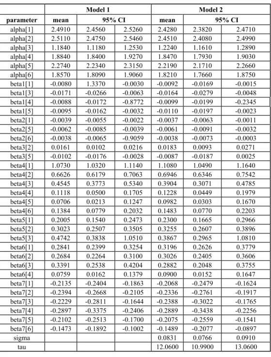
Table 4 – Results for Pneumonia.
Model 1 Model 2
parameter mean 95% CI mean 95% CI
alpha[1] 2.4910 2.4560 2.5260 2.4280 2.3820 2.4710
alpha[2] 2.5110 2.4750 2.5460 2.4510 2.4080 2.4990
alpha[3] 1.1840 1.1180 1.2530 1.2240 1.1610 1.2890
alpha[4] 1.8840 1.8400 1.9270 1.8470 1.7930 1.9030
alpha[5] 2.2740 2.2340 2.3150 2.2190 2.1710 2.2660
alpha[6] 1.8570 1.8090 1.9060 1.8210 1.7660 1.8750
beta1[1] -0.0080 1.3370 -0.0030 -0.0092 -0.0169 -0.0015 beta1[3] -0.0171 -0.0266 -0.0063 -0.0164 -0.0279 -0.0048 beta1[4] -0.0088 -0.0172 -0.8772 -0.0099 -0.0199 -0.2345 beta1[5] -0.0095 -0.0162 -0.0032 -0.0110 -0.0197 -0.0023 beta2[1] -0.0039 -0.0055 -0.0022 -0.0037 -0.0063 -0.0011 beta2[5] -0.0062 -0.0085 -0.0039 -0.0061 -0.0091 -0.0032 beta2[6] -0.0038 -0.0065 -0.9059 -0.0038 -0.0073 -0.0003
beta3[2] 0.0161 0.0102 0.0216 0.0183 0.0093 0.0271
beta3[5] -0.0102 -0.0176 -0.0028 -0.0087 -0.0187 0.0025
beta4[1] 1.0730 1.0320 1.1140 1.1080 1.0490 1.1640
beta4[2] 0.6626 0.6179 0.7063 0.6946 0.6346 0.7542
beta4[3] 0.4545 0.3773 0.5340 0.3904 0.3071 0.4785
beta4[4] 0.1118 0.0500 0.1705 0.1228 0.0449 0.1979
beta4[5] 0.0706 0.0213 0.1247 0.0982 0.0303 0.1670
beta4[6] 0.1384 0.0779 0.2032 0.1483 0.0770 0.2203
beta5[1] 0.2005 0.1540 0.2473 0.2300 0.1665 0.2966
beta5[2] 0.3023 0.2507 0.3505 0.3255 0.2607 0.3896
beta5[3] 0.4742 0.3838 1.0510 0.3867 0.2965 1.0810
beta6[1] 0.2841 0.2399 0.3254 0.3196 0.2626 0.3779
beta6[2] 0.2684 0.2264 0.3100 0.3026 0.2405 0.3606
beta6[3] 0.3391 0.2538 0.4204 0.2882 0.2048 0.3755
beta6[4] 0.0759 0.0162 0.1379 0.0900 0.0152 0.1647
beta7[1] -0.2135 -0.2404 -0.1863 -0.2068 -0.2479 -0.1624 beta7[2] -0.2394 -0.2668 -0.2105 -0.2336 -0.2761 -0.1917 beta7[3] -0.2229 -0.2811 -0.1644 -0.2388 -0.3022 -0.1765 beta7[4] -0.2897 -0.3375 -0.2406 -0.2889 -0.3438 -0.2256 beta7[5] -0.2102 -0.2513 -0.1700 -0.2075 -0.2559 -0.1541 beta7[6] -0.1473 -0.1892 -0.1002 -0.1489 -0.2077 -0.0897
sigma 0.0831 0.0766 0.0910
Table 5 – Results for Diabetes.
Model 1 Model 2
parameter mean 95% CI mean 95% CI
alpha[1] -1.6470 -1.9240 -1.3800 -0.0699 -0.2068 0.0664 alpha[2] -1.0400 -1.2690 -0.8150 0.0429 -0.0853 0.1808
alpha[3] -0.5496 -0.7192 -0.3901 0.1689 0.0493 0.2930
alpha[4] 0.1163 -0.0019 0.2310 0.4855 0.3779 0.5847
alpha[5] -0.7597 -0.9449 -0.5720 0.1123 -0.0118 0.2286
alpha[6] -0.5228 -0.6923 -0.3498 0.1843 0.0682 0.2932
alpha[7] -0.3456 1.3370 -0.1911 0.2451 0.1282 0.3676
alpha[8] -0.0898 -0.2278 0.0418 0.3674 0.2646 0.4815
alpha[9] 1.7830 1.7280 1.8320 1.9030 1.8430 1.9610
alpha[10] 0.7429 0.6579 0.8280 0.9402 0.8555 1.0270
beta1[1] 0.0218 -0.0261 0.0730 0.0733 0.0311 0.1175
beta1[2] 0.0155 -0.0223 0.0534 0.0524 0.0172 0.0876
beta1[5] 0.0110 -0.0206 0.0450 0.0415 0.0102 0.0757
beta1[7] 0.0203 -0.0034 0.0456 0.0383 0.0130 0.0629
beta2[1] 0.0135 -0.0042 0.0303 -0.0219 -0.0369 -0.0067 beta2[2] -0.0011 -0.0148 0.0138 -0.0201 -0.0325 -0.0072 beta2[3] 0.0712 -0.0100 0.0105 -0.0123 -0.0217 -0.0029 beta2[4] -0.0018 -0.0086 0.0052 -0.0079 -0.0152 -0.8768 beta2[5] -0.6925 -0.0127 0.0103 -0.0164 -0.0277 -0.0050 beta2[6] -0.9598 -0.0113 0.0091 -0.0131 -0.0230 -0.0034 beta2[9] -0.0037 -0.0070 -0.5364 -0.0061 -0.0099 -0.0021 beta3[1] 0.0877 0.0318 0.1443 -0.0584 -0.1040 -0.0091 beta3[2] -0.0110 -0.0562 0.0349 -0.0827 -0.1178 -0.0438 beta3[5] 0.0216 -0.0170 0.0623 -0.0421 -0.0784 -0.0071 beta3[6] 0.0054 -0.0288 0.0386 -0.0412 -0.0747 -0.0084 beta3[9] 0.0105 0.0002 0.0210 0.0022 -0.0104 0.0151 beta4[1] -0.2067 -0.5690 0.1768 -1.8020 -2.1130 -1.5110 beta4[2] -0.3215 -0.6279 -0.0149 -1.4580 -1.7240 -1.2070 beta4[3] -0.1366 -0.3641 0.1161 -0.8981 -1.1040 -0.6902 beta4[4] 0.0120 -0.1519 0.1718 -0.3875 -0.5326 -0.2338 beta4[5] -0.0587 -0.3339 0.1923 -0.9796 -1.1880 -0.7587 beta4[6] -0.0108 -0.2304 0.2210 -0.7614 -0.9691 -0.5608 beta4[7] 0.0069 -0.1926 0.2016 -0.6202 -0.8078 -0.4329 beta4[8] -0.0195 -0.1980 0.1605 -0.5092 -0.6716 -0.3417 beta4[9] 0.0040 -0.0670 0.0779 -0.1452 -0.2297 -0.0654 beta4[10] -0.0154 -0.1261 0.0957 -0.2455 -0.3656 -0.1251
beta5[6] -0.0627 -0.3265 0.1999 -0.9511 -1.1610 -0.7377 beta5[7] -0.1053 -0.3339 0.1105 -0.8536 -1.0650 -0.6572 beta5[8] -0.0370 -0.2351 0.1558 -0.6165 -0.7916 -0.4338 beta5[9] -0.0963 -0.1694 -0.0191 -0.2770 -0.3659 -0.1892 beta5[10] -0.1039 -0.2278 0.0143 -0.3731 -0.5101 -0.2426
beta6[1] -0.0698 -0.4282 0.2977 -1.3180 -1.6000 -1.0460 beta6[2] 0.0609 -0.2264 0.3378 -0.8737 -1.1210 -0.6319 beta6[3] -0.1546 -0.3825 0.0896 -0.7803 -0.9878 -0.5850 beta6[4] 0.1327 -0.0208 0.2948 -0.2023 -0.3565 -0.0454 beta6[5] -0.0165 -0.2502 0.2377 -0.7749 -0.9980 -0.5539 beta6[6] -0.0971 -0.3453 0.1444 -0.7143 -0.9327 -0.5093 beta6[7] 0.0859 -0.1055 0.2763 -0.4392 -0.6152 -0.2600 beta6[8] -0.0790 -0.2636 0.1042 -0.4871 -0.6702 -0.3245 beta6[9] 0.0044 -0.0619 0.0721 -0.1277 -0.2101 -0.0453 beta6[10] 0.0313 -0.0857 0.1493 -0.1619 -0.2826 -0.0477
beta7[1] -0.1401 -0.4351 0.1371 -0.6458 -0.9146 -0.3786 beta7[2] -0.3052 -0.5354 -0.0715 -0.6206 -0.8253 -0.4089 beta7[3] -0.3733 -0.5600 -0.1805 -0.5779 -0.7584 -0.4031 beta7[4] -0.3502 -0.4679 -0.2328 -0.4557 -0.5785 -0.3348 beta7[5] -0.7234 -0.9428 -0.5008 -0.9643 -1.1950 -0.7426 beta7[6] -0.6831 -0.8721 -0.4831 -0.8745 -1.0640 -0.6787 beta7[7] -0.5003 -0.6489 -0.3470 -0.6595 -0.8329 -0.5119 beta7[8] -0.5074 -0.6505 -0.3544 -0.6335 -0.7828 -0.4855 beta7[9] -0.3474 -0.3993 -0.2925 -0.3871 -0.4487 -0.3193 beta7[10] -0.2638 -0.3536 -0.1674 -0.3206 -0.4225 -0.2245
sigma 0.1045 0.0921 0.1182
tau 9.6080 8.4630 10.8600
In all cases we observe that “Model 2” (presence of random effect) presents the best adjustment to the data using as the criterion the lowest value of the sum of squares of the differences s2
( )
v (observed – fitted).The DIC criterion also selects “Model 2”, except for the case of hospitalization due to diabetes. However, we decided for “Model 2” even for this case because the criterion of sum of squares of the differences provides a strong indication in favor of “Model 2” and in the case of hospitalization due to diabetes there is a large number days with zero hospitalization, which can invalidate the use of DIC criterion for model discrimination.
5. Discussion of Results
Considering the case of daily hospitalizations for chronic conditions and assuming that “Model 2” best fits the data, we have from table 2:
18
ˆ 0.165
β = − , that is, we observe that there is a decrease in the number of daily hospital admissions due to an increase in the average level of air pressure for this group. That is, low atmospheric pressure leads to an increase in hospital admissions due to chronic diseases.
(2) The average humidity in the i-th day is significant for groups 2, 6 and 8 (βˆ22=0.0036, i.e., higher humidity leads to an increase in daily admissions for chronic conditions for patients in group 2; for groups 6 and 8 we have βˆ26= −0.0062 and βˆ28= −0.00866, that is, higher daily average humidity leads to a decrease in the number of hospitalization due to chronic diseases).
(3) The average temperature in the i-th day is significantly positive (i.e., the increase in average daily temperature leads to an increase in the number of hospitalizations due to chronic diseases for under 10 years old persons (βˆ31=0.0404; βˆ32=0.0348 and
35
ˆ 0.0315
β = ).
(4) The fall is significant for all groups except 5 and 6 ([15,60) years old person). All effects are positive, except for group 4. (βˆ41=1,000; βˆ42=0.4968; βˆ43=0.2809;
44
ˆ 0.1687
β = − ; βˆ47=0.0922 and βˆ48=0.1092).
(5) The winter is significant for all groups except ages 60 and higher. The effect is positive for groups corresponding to persons less than 10 years old (βˆ51=0.2242;
52
ˆ 0.1010
β = ; βˆ53=0,1981) and negative for groups 5 and 6 (βˆ55= −0.1899 and
56
ˆ 0.2016
β = − ).
(6) The spring is significant for groups 1,2,3 and 4 (βˆ61=0.3699; βˆ62=0.1482;
63
ˆ 0.2904
β = , βˆ64= −0.2046). The effect is positive for groups 1, 2 and 3 (increase of admissions) and negative for group 4 (decrease of admissions).
(7) The Weekend (Saturday-Sunday) is significant for all groups except group 3, all with negative effect (βˆ71= −0.1616; βˆ72= −0.1855; βˆ74= −0.2969; βˆ75= −0.3060;
76
ˆ 0.2239
β = − ; βˆ77= −0.3113 and βˆ78= −0.3206).
Similarly, considering the case of hospitalization due to ischemic and assuming “Model 2”, we have the following results (see table 3) in a simplified form:
(1) The average pressure in the i-th day is significant only for groups 2 and 7.
12
ˆ 0.0245
β = and βˆ17 = −0.0159.
(2) The average humidity in the i-th day is significant only for group 2 (negative) and 7 (negative).
(3) The average temperature in the i-th day is significant only for group 7 (positive,
37
ˆ 0.0333
(4) The fall is significant negative for group 3. (βˆ43= −0.1487).
(5) The winter is significantly negative for groups 1, 2, 3 and 6.
(6) The spring is significant for all groups except for groups 3 and 4. The effect is negative for less than 40 years old persons and positive for 50 years old and older persons.
(7) The weekend (Saturday-Sunday) is significantly negative for all groups.
In the case of pneumonia considering “Model 2”, we have (see table 4):
(1) The average pressure in the i-th day is significantly negative for groups 1, 3, 4 and 5.
(2) The average humidity in the i-th day is significantly negative for groups 1, 5 and 6 (less than one year old and 45 years old or older persons).
(3) The average temperature in the i-th day is significant for group 2. βˆ32=0.0183.
(4) The autumn is significantly positive for all groups.
(5) The winter is significantly positive for groups 1, 2 and 3 (less than 10 years old groups).
(6) The spring is significantly positive for groups 1, 2, 3 and 4 (less than 45 years old groups).
(7) The weekend (Saturday-Sunday) is significantly negative for all groups.
In the case of diabetes also assuming “Model 2”, we have (see table 5):
(1) The average pressure in the i-th day is significantly positive for groups 1, 2, 5 and 7.
(2) The average humidity in the i-th day is significantly negative, except for groups 7, 8 and 10.
(3) The average temperature in the i-th day is significantly negative for groups 1, 2, 5 and 6.
(4) The autumn is significantly negative for all groups.
(5) The winter is significantly negative for all groups.
(6) The spring is significantly negative for all groups.
(7) The weekend (Saturday-Sunday) is significantly negative for all groups.
In view of these results, we can reach the following overall conclusions:
1. In general, all the variables are influencing the average number of admissions.
3. The significance of dummy variables corresponding to the seasons and the weekend indicates that seasonal patterns also have influence on the behavior of the number of hospitalizations.
4. The meteorological conditions have more influence in groups corresponding to children and elderly.
Acknowledgments
This work was partially supported by CNPq, CAPES and FAPESP. The authors thank the laboratory EPIFISMA (IMECC-UNICAMP).
References
(1) Albert, J.H. (1992). Bayesian analysis of a Poisson random effect model for home run hitters. The American Statistician, 16, 246-253.
(2) Albert, J.H. & Chib, S. (1993). Bayesian analysis of binary and polychotonious response data. Journal of American Statistical Association, 88, 669-679.
(3) Achcar, J.A.; Coelho-Barros, E. & Martinez, E.Z. (2008). Statistical analysis for longitudinal counting data in the presence of a covariate considering different “frailty” models. Brazilian Journal of Probability and Statistics, 22, 183-205.
(4) Chib, S. & Greenberg, E. (1995). Understanding the Metropolis-Hastings algorithm. The American Statistician, 49, 327-335.
(5) Chib, S.; Greenberg, E. & Winkelmann, R. (1998). Posterior simulation and Bayes factors in panel count data models. Journal of Econometrics, 86, 33-54.
(6) Clayton, David G. (1991). A Monte Carlo method for Bayesian inference in frailty models. Biometrics, 47, 467-485.
(7) Crouchley, R. & Davies, R.B. (1999). A comparison of population average and random effects models for the analysis of longitudinal count data with baseline information. Journal of the Royal Statistical Society, A, 162, 331-347.
(8) DATASUS – Department de Informatics do SUS, Secretaria Executiva, Ministério da SaúdeVersão 1.6c – ©1993 by CBCD and DATASUS. In: <www.datasus.gov.br/> Acessed on October 13, 2008.
(9) Dunson, D.B. (2000) Bayesian latent variable models for clustered mixed outcomes. Journal of the Royal Statistical Society, B, 62, 335-366.
(10) Dunson, D.B. (2003) Dynamic latent trail models for multidimensional longitudinal data. Journal of the American Statistical Association, 85, 385-409.
(11) Dunson, D.B. & Herrinng, A.H. (2005). Bayesian latent variable models for mixed discrete outcomes. Biostatistics, 6, 11-25.
(12) Gelfand, A.E. & Smith, A.F.M. (1990). Sampling-based approaches to calculating marginal densities. Journal of the American Statistical Association, 85, 385-409.
(14) Korsgaard, I.R. & Andersen, A.H. (1998). The additive genetic gamma frailty model. Scandinavian Journal of Statistics, 25, 255-269.
(15) Legler, J.M. & Ryan, L.M. (1997). Latent variable models for teratogenesis using multiply binary outcomes. Journal of American Statistical Association, 92, 13-20.
(16) Li, H.Z. (2002). An additive genetic gamma frailty model for linkage analysis of diseases with variable age of owsed using nuclear families. Lifetime Data Analysis, 8, 315-334.
(17) Moustaki, I. & Knott, M. (2000). Generalized latent trail models. Psychometrika, 65, 391-411.
(18) Petersen, J.H. (1998). An Additive frailty model for correlated life times. Biometrics,
54, 646-661.
(19) Sammel, M.D.; Ryan, L.M. & Legler, J.M. (1997). Latent variable models and mixed discrete and continuous outcomes. Journal of the Royal Statistical Society, B, 59,
667-678.
(20) Spiegelhalter, D.J.; Best, N.G.; Carlin, B.P. & Vander Linde, A. (2002). Bayesian measures of model complexity and fit (with discussion). Journal of the Royal Statistical Society, B, 64, 583-639.