Comput. Appl. Math. vol.28 número1

ISSN 0101-8205 www.scielo.br/cam

Central schemes for porous media flows

E. ABREU1, F. PEREIRA2 and S. RIBEIRO3

1_{Instituto Nacional de Matemática Pura e Aplicada,}

22460-320 Rio de Janeiro, RJ, Brazil

2_{Department of Mathematics and School of Energy Resources,}

University of Wyoming, Laramie, WY 82071-3036, USA

3_{Departamento de Ciências Exatas, Universidade Federal Fluminense,}

27255-250 Volta Redonda, RJ, Brazil

E-mails: [email protected] / [email protected] / [email protected]

Abstract. We are concerned with central differencing schemes for solving scalar hyperbolic conservation laws arising in the simulation of multiphase flows in heterogeneous porous media. We compare the Kurganov-Tadmor (KT) [3] semi-discrete central scheme with the Nessyahu-Tadmor (NT) [27] central scheme. The KT scheme uses more precise information about the local speeds of propagation together with integration over nonuniform control volumes, which contain the Riemann fans. These methods can accurately resolve sharp fronts in the fluid saturations without introducing spurious oscillations or excessive numerical diffusion. We first discuss the coupling of these methods with velocity fields approximated by mixed finite elements. Then, numerical simulations are presented for two-phase, two-dimensional flow problems in multi-scale heterogeneous petroleum reservoirs. We find the KT scheme to be considerably less diffusive, particularly in the presence of high permeability flow channels, which lead to strong restrictions on the time step selection; however, the KT scheme may produce incorrect boundary behavior.

Mathematical subject classification: Primary: 35L65; Secondary: 65M06.

Key words:hyperbolic conservation laws, central differencing, two-phase flows.

1 Introduction

We are concerned with high resolution central schemes for solving scalar hyper-bolic conservation laws arising in the simulation of multiphase flows in multi-dimensional heterogeneous petroleum reservoirs.

Many of the modern high resolution approximations for nonlinear conserva-tion laws employ Godunov’s appoach [35] orREA(reconstruct, evolve, average) algorithm, i.e., the approximate solution is represented by a piecewise polyno-mial which isReconstructed from the Evolving cellAverages. The two main classes of Godunov methods are upwind and central schemes.

The Lax-Friedrichs (LxF) scheme [33] is the canonical first order central scheme, which is the forerunner of all central differencing schemes. It is based on piecewise constant approximate solutions. It also enjoys simplicity, i.e., it does not employ Riemann solvers and characteristic decomposition. Unfortunately the excessive numerical dissipation in the LxF recipe (of orderO((1X)2/1t))

yields poor resolution, which seems to have delayed the development of high resolution central schemes when compared with the earlier developments of the high resolution upwind methods. Only in 1990 a second order generaliza-tion to the LxF scheme was introduced by Nessyahu and Tadmor (NT) [27]. They used a staggered form of the LxF scheme and replaced the first order piecewise constant solution with a van Leer’s MUSCL-type piecewise linear second order approximation [8]. The numerical dissipation in this new central scheme has an amplitude of orderO((1X)4/1t). When applying these methods

two-phase flows with a much lower numerical diffusion, even in the presence of a highly heterogeneous porous media.

The goals of this paper are (i) to discuss the coupling of NT and KT schemes to velocity fields approximated by Raviart-Thomas mixed finite element method (See [30]), and (ii) to compare the KT semi-discrete central scheme with the NT central scheme for numerical simulations of phase, incompressible, two-dimensional flows in heterogeneous formations. Both methods can accurately resolve sharp fronts in the fluid saturations without introducing spurious oscil-lations or excessive numerical diffusion.

Our numerical experiments indicate that the KT scheme is considerably less diffusive, particularly in the presence of viscous fingers, which lead to strong restrictions on the time step selection. On the other hand the KT scheme may produce incorrect boundary behavior in a typical two-dimensional geometry used in the study of porous media flows: the quarter of a five spot.

Numerous methods have been introduced to solve two-phase flow problems in porous media. Among eulerian-lagrangian procedures we mention the Modi-fied Method of Characteristics [25, 29], the ModiModi-fied Method of Characteristics with Adjusted Advection [22], the Locally Conservative Eulerian Lagrangian Method [23] and Eulerian Lagragian Localized Adjoint Methods [26]. Addi-tional techniques, to name just a few, include higher–order Godunov schemes [10], the front-tracking method [7], the streamline method [32, 34] the streamline upwind Petrov-Galerkin method (SUPG) [1, 4] and a second-order TVD-type finite volume scheme [31] (this procedure aims at the modeling of flow through geometrically complex geological reservoirs). Each of these procedures has ad-vantages and disadad-vantages. We refer the reader to [28, 23] and references cited there for a discussion of these methods.

We remark that central schemes are particularly interesting for the numeri-cal simulation of multiphase flow problems in porous media because they have been formulated to solve hyperbolic systems; this is not the case for several of the procedures mentioned above, which have been developed only for scalar equations.

the two-dimensional magnetohydrodynamics (MHD) equations and to study the Orszag-Tang vortex system, which describes the transition to supersonic turbu-lence for the equations of MHD in two space dimensions (see [9] and [20]), to mention just a couple of them.

This paper is organized as follows. In Section 2, we discuss our strategy for solving numerically the model for two-phase, immiscible and incompressible displacement in heterogeneous porous media considered here. In Section 3, we discuss the application of central differencing schemes to porous media flows. In Section 4, we present the computational solutions for the model problem considered here and our conclusions.

2 Numerical approximation of two-phase flows

We consider a model for two-phase immiscible and incompressible displace-ment in heterogeneous porous media. The governing equations are strongly nonlinear and lead to shock formation, and with or without diffusive terms they are of practical importance in petroleum engineering [15, 24]. See also [21] and the references therein for recent studies for the scale-up problem for such equa-tions. The conventional theoretical description of two-phase flow in a porous medium, in the limit of vanishing capillary pressure, is via Darcy’s law coupled to the Buckley-Leverett equation. The two phases will be referred to as water and oil, and indicated by the subscriptswando, respectively. Without sources

or sinks and neglecting the effects of capillarity and gravity, these equations read (See [15] for more details)

∇ ∙v=0, v= −λ(s)K(x)∇p, (1)

∂s

∂t + ∇ ∙(f(s)v)=0, (2)

Here,vis the total seepage velocity,sis the water saturation,K(x)is the absolute

permeability, and pis the pressure. The constant porosity has been scaled out

by a change of the time variable. The total mobility,λ(s), and water fractional

flow function, f(s), are defined in terms of the relative permeabilitieskr i(s)and phase viscositiesμi by

λ(s)= krw(s)

μw

+ kr o(s)

μo

, f(s)= krw(s)/μw

2.1 Operator splitting for two-phase flow

An operator splitting technique is employed for the computational solution of the saturation equation (2) and the pressure equation (1) in which they are solved sequentially with possibly distinct time steps. This splitting scheme has proved to be computationally efficient in producing accurate numerical solutions for two-phase flows. We refer the reader to [22] and references therein for more details on the operator splitting technique; see also [16, 14, 17, 18] and [5] for applications of this strategy to three phase flows taking into account capillary pressure (diffusive effects).

Typically, for computational efficiency larger time steps are used for the pressure-velocity calculation (Equation 1) than for the convection calculation (Equation 2). Thus, we introduce two time steps: 1tc for the solution of the hyperbolic problem for convection, and1tp for the pressure-velocity calcula-tion so that1tp≥1tc. We remark that in practice variable time steps are always useful, especially for the convection micro-steps subject dynamically to aC F L

condition.

For the pressure solution we use a (locally conservative) hybridized mixed finite element discretization equivalent to cell-centered finite differences [21, 22], which effectively treats the rapidly changing permeabilities that arise from stochastic geology and produces accurate velocity fields. The pressure and Darcy velocity are approximated at times tm = m1tp, m = 0,1,2, . . ..

The linear system resulting from the discretized equations is solved by a pre-conditioned conjugate gradient procedure (PCG) (See [22] and the references therein). The saturation equation is approximated at timestm

κ =tm+κ1tcfor

tm <t_κm ≤tm+1. We remark that we must specify the water saturation att =0.

3 Central differencing schemes for porous media flows

problem (Eq. (1)), we use the lowest order Raviart-Thomas [30] locally conser-vative mixed finite elements. These central schemes enjoy the main advantage of Godunov-type central schemes: simplicity, i.e., they employ neither characteris-tic decomposition nor approximate Riemann solvers. This makes them universal methods that can be applied to a wide variety of physical problems, including hyperbolic systems. In the following sections we will discuss the main ideas of the NT and KT central schemes coupled to the mixed finite element discretiza-tion mendiscretiza-tioned above. We will not repeat here all the details involved in the development of the NT and KT schemes; instead, we refer the reader to [27] and [3] for this material.

3.1 The Nessyahu-Tadmor scheme for two-phase flows

Consider the following scalar hyperbolic conservation law,

∂s ∂t +

∂

∂x

x

vf(s)+ ∂

∂y

y

vf(s)=0, (3)

subject to prescribed initial data,s(x,y,0) = S0(x,y). Herexv = xv(x,y,t) andy_{v =} y_{v(x,y,t)denote thex−and y−components of the velocity fieldv} (see Eq. 1). To approximate (3) by the NT scheme, we begin with a piecewise constant solution of the form

X

j,k

Sκ_j,kχj,k(x,y), where S

κ

j,k := S xj,yk,tκm

is the approximate cell average att = tm

κ associated with the cellCj,k = Ij×

Ik = [xj−1/2,xj+1/2] × [yk−1/2,yk+1/2]andχj,k(x,y)is a characteristic function of the cellCj,k.

We first reconstruct a piecewise linear approximation of the form

s x,y,t_κm =X j,k

eSκ_j,k(x,y)χj,k(x,y)

= X j,k



Sκ_j,k+ S

κ

j,k ´

1X (x−xj)+ Sκ

j,k `

1Y (y−yk)



χj,k(x,y)

xj−1/2≤ x ≤xj+1/2, yk−1/2≤ y≤ yk+1/2.

In Eq. (4), the discrete slopes along thex andy directions satisfy

Sκ

j,k´

1X =

∂

∂xs(x =xj,y =yk,t

κ_{)+O(1X) (5a)}

Sκ_j,k`

1Y =

∂

∂ys(x =xj,y =yk,t κ

)+O(1Y), (5b)

to guarantee second-order accuracy.

The reconstruction (4) retains conservation, i.e.:

1

1X1Y

Z xj+1/2

xj−1/2

Z yk+1/2

yk−1/2

eSκ(x,y)d xd y=Sκ_j,k. (6)

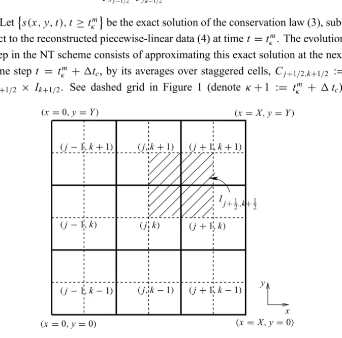
Lets(x,y,t),t≥tm

κ be the exact solution of the conservation law (3),

sub-ject to the reconstructed piecewise-linear data (4) at timet =t_κm. The evolution

step in the NT scheme consists of approximating this exact solution at the next time stept = t_κm +1tc, by its averages over staggered cells, Cj+1/2,k+1/2 :=

Ij+1/2 × Ik+1/2. See dashed grid in Figure 1 (denote κ+1 := tκm + 1tc).

( , + )

( − , + ) ( + , + )

( = , = ) ( = , = )

( = , = ) ( = , = )

( − , ) ( , ) ( + , )

( − , − ) ( , − ) ( + , − )

+ , +

Let

Sκ_j++11₂,k+1₂ =

1

1X1Y

Z

Cj+1/2,k+1/2

s x,y,t_κm+1tc

d xd y

= 1

1X1Y

Z xj+1

xj

Z yk+1

yk

s x,y,t_κm+1tc

d xd y. (7)

xj ≤x ≤xj+1, yk ≤ y ≤ yk+1

These new staggered cell averages are obtained by integrating the conservation law (3) over the control volumesCj+1/2,k+1/2× [tκm,tκm +1tc] following the

same manipulations as described in [19] (denoteαx ≡ ₁1t_Xc andαy ≡ 1₁t_Yc):

Sκ_j+₊₁1_/2,k+1/2 = 1

1X1Y

Z

Cj+1/2,k+1/2

s x,y,t_κm+1tc

d xd y

− αx

1X1Y

Z t_κm+1tc

tm

κ

Z yk+1

yk

h

x_v(x

j+1,y, τ ) f(s(xj+1,y, τ )

−x_v(x

j,y, τ ) f(xj,y, τ )

i

d y dτ

− αy

1X1Y

Z tκm+1tc

tm

κ

Z xj+1

xj

h

y_v(x,y

k+1, τ ) f(s(x,yk+1, τ )

−y_v(x

,yk, τ ) f(x,yk, τ )

i

d x dτ

.

(8)

The cell average

Z

C j+1/2,k+1/2

s x,y,t_κm +1tc

d xd y

has contributions from the four cells Cj,k, Cj+1,k, Cj+1,k+1, and Cj,k+1: Z

Cj+1/2,k+1/2

s x,y,t_κmd xd y =

Z

Cj+1/2,k+1/2∩Cj,k

eSκ_j,k(x,y) +

Z

Cj+1/2,k+1/2∩Cj,k+1 eSκ_j,k+1(x,y)

+

Z

Cj+1/2,k+1/2∩Cj+1,k

eSκ_j+1,k(x,y) +

Z

Cj+1/2,k+1/2∩Cj+1,k+1 eSκ_j+1,k+1(x,y)

Computing these integrals exactly yields

Sκ_j+1₂,k+1₂ =

1 4 S

κ

j,k+S

κ

j,k+1+S

κ

j+1,k+S

κ

j+1,k+1

+ 1 16

h

Sκ_j,k´ + Sκ_j,k+1´

− Sκ_j+1,k´

− Sκ_j+1,k+1´

+ Sκ_j,k` − Sκ<sub>j,k</sub>+1`

+ Sκ_j+1,k`

− Sκ_j+1,k+1`

i

.

(10)

To approximate the four flux integrals on the right hand side of (8), we use the second-order rectangular quadrature rule for the spatial integration and the mid-point quadrature rule for second-order approximation of the temporal integrals. For instance, lettingκ+1/2 betm

κ +1tc/2,

αx

1X1Y

Z tκm+1tc

tm

κ

Z yk+1

yk x_v(x

j+1,y, τ ) f(s(xj+1,y, τ ))d y dτ ≈ αx

2

h

x_vκ+1/2 j+1,k f s

κ+1/2 j+1,k

+x_vκ+1/2 j+1,k+1 f s

κ+1/2 j+1,k+1

i

, (11a)

αy

1X1Y

Z t_κm+1tc

tm

κ

Z xj+1

xj

y_v(x,y

k+1, τ ) f(s(x,yk+1, τ ))d y dτ

≈ αy 2

h

y

vκ_j,+_k1₊/₁2 f sκ_j,+_k+1/12

+yvκ_j+₊1_1,/_k2₊₁ f sκ_j++11,/k2+1

i

. (11b)

Since these midvalues are computed at the center of the cells, Cj,k, where the solution is smooth, provided an appropriate CFL condition is observed, we can use Taylor expansion together with the conservation law (3) to get

sκ_j,+_k1/2 = Sκ_j,k− αx 2

x_vκ

j,k f

κ

j,k´

−αy 2

y_vκ

j,k f

κ

j,k`

. (12)

Here, fκ

j,k´

and fκ

j,k`

are one-dimensional discrete slopes in the x and y

directions, respectively. They satisfy the conditions

fκ_j,k´

1X =

∂

∂x f s(x =xj,y= yk,t κ

)+O(1X) (13a)

fκ

j,k `

1Y =

∂

∂y f s(x =xj,y= yk,t

in order to produce a second order scheme for the approximation of (3). To avoid spurious oscillations, it is essential to reconstruct the discrete derivatives given by Equations (5) and (13) with built-in nonlinear limiters. In this work we use the following MinMod limiter

(Sx)κj,k ≈ MMθ

1 1x

n

Sκj−1,k,S

κ

j,k,S

κ

j+1,k

o

:= MM θ1S

κ

j+1/2,k

1x ,

1Sκ_j−1/2,k−1Sκ_j+1/2,k

21x , θ

1Sκ_j−1/2,k

1x

!

; (14a)

(fx)κj,k ≈ MMθ

1 1x

n

f_jκ−1,k, f

κ

j,k, fjκ+1,k

o

:= MM θ1f

κ

j+1/2,k

1x ,

1fκ

j−1/2,k−1fjκ+1/2,k

21x , θ

1fκ

j−1/2,k 1y

!

, (14b)

where1 is the centered difference,1Sκ

j+1/2,k = S

κ

j+1,k −S

κ

j,k. We refer the reader to [27] and [3] and the references therein for the various options for the form of such discrete derivatives.

In our sequential scheme, when solving for the saturation in time, the total velocityvis given by the solution of the velocity-pressure equation. Recall that the solution of Eq. (1) is approximated the lowest order Raviart-Thomas mixed finite element method. Thus, the computed total velocityvis discontinuous at the vertices of the original non-staggered grid cells. This constitutes a difficulty for the staggered scheme (8), which requires the values of the total velocityv at these vertices at every other time step. To avoid this difficulty we use the non-staggered version of the NT scheme.

To turn the staggered scheme (8) into a non-staggered scheme, we re-average the reconstructed values of the underlying staggered scheme, thus recovering the cell averages of the central scheme over the original non-staggered grid cells. First we reconstruct a piecewise bilinear interpolant at the time stepκ +1 :=

tm

κ +1tc

eSκ_j++₁1_/2,k+1/2(x,y) = Sκ_j++11/2,k+1/2+

(Sκ_j++₁1_/2,k+1/2´)

1X (x −xj+1/2)

+ S

κ+1

j+1/2,k+1/2`

1Y (y−yk+1/2) xj ≤x ≤xj+1, yk ≤ y≤ yk+1,

as in Equation (4), through the staggered cell averages given by (8), and re-average it over the original grid cells, giving the following non-staggered scheme:

Sκj,+k1 = 1 4 S

κ+1

j−1/2,k−1/2+S κ+1

j−1/2,k+1/2+S κ+1

j+1/2,k−1/2+S κ+1

j+1/2,k+1/2

+ 1 16

h

Sκ_j−+₁1_/2,k−1/2´ + Sκ_j−+₁1_/2,k+1/2´

− Sκ_j++₁1_/2,k−1/2´ − Sκ_j++₁1_/2,k+1/2 i´

+ 1 16

h

Sκ_j−+11/2,k−1/2`

− Sκ_j−+11/2,k+1/2`

+ Sκ_j++11/2,k−1/2`

− Sκ_j++11/2,k+1/2`

i

.

3.2 The Kurganov-Tadmor scheme for two-phase flows

The first multidimensional extension of the KT scheme was presented in [3]. This extension used the dimension by dimension approach, that is, the numeri-cal fluxes computed along thexandydirections are viewed as a generalization of

the one-spatial-dimension numerical fluxes. This approach consists of the fol-lowing steps: at each time steptm

κ and at each cell Ij,k,

(i) Compute the difference of the one-dimensional numerical flux in one spa-tial dimension in thexdirection keepingyconstant and equal toyk. Denote this difference by

Fx_j+1/2,k(t):= H x

j+1/2,k(t)−H x

j−1/2,k(t)

1X .

The numerical flux Hx_j+1/2,k(t) is

Hx

j+1/2,k(t) := 1 2

h

x_v

j+1/2,k(t) f S+_j+1/2,k(t)

+x_v

j+1/2,k(t) f S−j+1/2,k(t)

i

− a x

j+1/2,k(t) 2

h

S+_j+1/2,k(t)−S−_j+1/2,k(t)i,

where

S+_j+1/2,k(t) = eSj+1,k(xj+1/2,yk,t) = Sj+1,k(t)−

1X

2 (Sx)j+1,k(t) and

S−_j+1/2,k(t) = eSj,k(xj+1/2,yk,t) = Sj,k(t)+

1X

2 (Sx)j,k(t)

(17)

are the corresponding right and left intermediate values of eS(x,tκ_{) at} (xj+1/2,yk).

The local speed of wave propagationax_j+1/2,k(t)is estimated at the cell boundaries(xj+1/2,yk)as the upper bound

ax_j+1/2,k(t)=max_ω

|xvj+1/2,k(t) f′(ω)| , (18) whereωis a value betweenS+_j+1/2,k(t)andS−_j+1/2,k(t). The velocity field used in the KT scheme is obtained directly from the Raviart-Thomas space on the cell edges:

x_v

j+1/2,k(t):=(vr)j k(t), xvj−1/2,k(t):=(vl)j k(t),

wherevr andvlstand for the velocity on the one-dimensional “right” and “left” faces of the cells.

(ii) Analogously, compute the difference of the one-dimensional numerical flux in theydirection keepingxconstant and equal toxj. This difference is denoted by

F_jy_,k+1/2(t):= H y

j,k+1/2(t)−H y

j,k+1/2(t)

1Y .

The one dimensional numerical flux in theydirection is

H_jy_,k+1/2(t) := 1 2

h

y_v

j,k+1/2(t) f S+j,k+1/2(t)

+y_v

j,k+1/2(t) f S−j,k+1/2(t)

i

− a y

j,k+1/2(t)

2

h

S+_j,k+1/2(t)−S−_j,k+1/2(t)i.

In a similar way, the correspondent “up” and “down” intermediate values ofeS(x,tκ_)at(x

j,yk+1/2)are

S+_j,k+1/2(t) = Sj,k+1(t)− 1Y

2 (Sy)j,k+1(t) and

S−_j,k+1/2(t) = Sj,k(t)+

1Y

2 (Sy)j,k(t).

The local speed of wave propagationay_j,k+1/2(t)in they direction is

esti-mated at the cell boundaries(xj,yk+1/2)as the upper bound ay_j+1/2,k(t)=max

ω

|yvj+1/2,k(t) f′(ω)| , (20) whereωis a value between S+_j,k+1/2(t)andS−j,k+1/2(t). Analogously the velocity field in the y direction is obtained directly from the

Raviart-Thomas space on the cell edges:

x

vj,k+1/2(t):=(vu)j k(t), xvj,k−1/2(t):=(vd)j k(t),

wherevu andvd stand for the velocity on the “upper” and “lower” faces of the cells.

(iii) The cell averageSκj,+k1in the next time steptκm +1tc is then the solution of the following differential equation

d

dtSj,k(t) = − F

x

j+1/2,k(t)+F y

j,k+1/2(t)

= − H x

j+1/2,k(t)−Hjx−1/2,k(t)

1X (21)

− H y

j,k+1/2(t)−H

y

j,k+1/2(t)

1Y ,

The numerical derivatives are computed using the MinMod limiter given by Equation (14). In our numerical experiments, the parameterθ assumes values

1< θ <1.8.

forward Euler scheme can be used, it may be advantageous to use higher order discretizations in numerical simulations. The numerical examples presented below use third-order Runge-Kutta ODE solvers based on convex combinations of forward Euler steps. See [12] and [13] for more details on a whole family of such schemes.

4 Two-dimensional numerical experiments

We present and compare the results of numerical simulations of two-dimensional, two-phase flows associated with two distinct flooding problems using the KT and NT schemes.

In all simulations, the reservoir contains initially 79% of oil and 21% of water. Water is injected at a constant rate of 0.2 pore volumes every year. The viscosity

of oil and water used are μo = 10.0c P and μw = 0.05c P. The relative permeabilities are assumed to be:

kr o(s)= 1−(1−sr o)−1s

2

, krw(s)= 1−srw

−2

s−srw

2

,

where sr o = 0.15 and srw = 0.2 are the residual oil and water saturations,

respectively.

For the heterogeneous reservoir studies we consider a scalar absolute perme-ability field K(x) taken to be log-normal (a fractal field, see [6] and [21] for

more details) with moderately large heterogeneity strength. The spatially vari-able permeability field is defined on a 256×64 grid with three different values of the coefficient of variationC V (C V =0.5, 1.2, 2.2) given by the ratio between

the standard deviation and the mean value of the permeability field.

We now discuss the simulations in the slab geometry. We consider two-dimensional flows in a rectangular, heterogeneous reservoir (slab geometry)

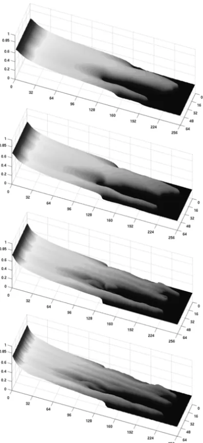
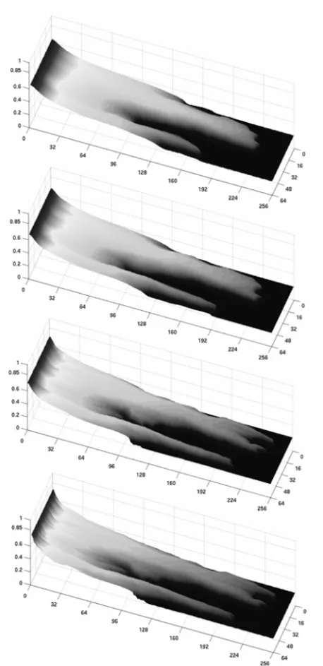
Figures 3, 4, and 5 refer to a comparative study of the NT and KT schemes, showing the water saturation surface plots after 275, 250 and 225 days of sim-ulation for the three different CV values (C V =0.5,1.2,and 2.2). The results

obtained with the NT scheme were computed using three computational grid: the coarsest grid with 256×64 cells, and two levels of refinement denoted by NTr and NTrr with 512×128 and 1024×256 cells, respectively (See the first three pictures from top to bottom of Figures 3, 4, and 5). At the same time, the bottom pictures in those figures are the results presented by the KT dimension by dimension scheme on the coarsest computational grid of 256×64 cells.

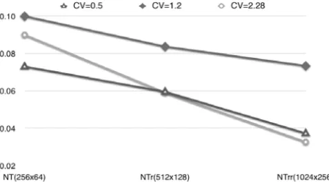
Figure 2 – The numerical differences in L2_{norm between the solution of the KT scheme}

and the solutions of the NT scheme using three computional grids. As we refine the grid of NT scheme, the differences become smaller.

For each heterogeneity, we computed the difference between the results pro-duced by the NT scheme in the three computational grids with the corresponding result produced by the KT scheme in the coarsest grid. We consider the solution of the NT scheme in the finer grid as the reference solution. The differences are then computed using the L2_{norm relative to this reference solution as follows}

numerical differences= kF−Gk2 kNTrrk2

. (22)

HereFstands for the KT solution andGfor a NT solution. The graph in Figure 2

Figure 3 – Water saturation surface plots after 275 days of simulation in a heterogeneous reservoir having 256 m×64 m, withC V =0.5 and viscosity ratio 20. The first three pictures from top

NT scheme in the finest grid. These differences indicate that one has to refine twice the grid used in the NT scheme to produce an equivalent solution to the one produced by the KT scheme using the coarsest grid.

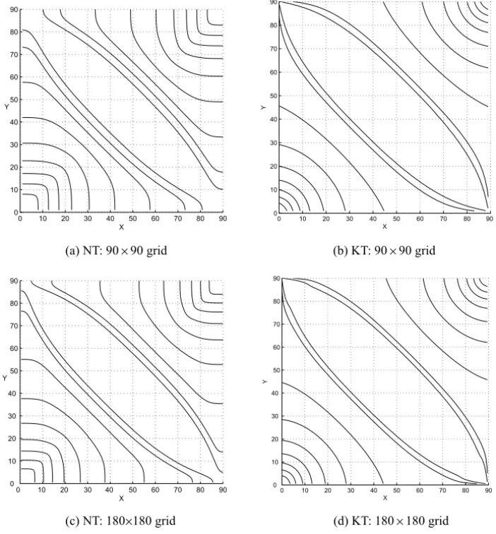
We now turn to the discussion of the set of simulations performed in a five-spot pattern. In case of a five-spot flood discretized by a diagonal grid (Figure 6), injection takes place at one corner and production at the diametrically opposite corner; no flow is allowed across the entirety of the boundary. In case of a five-spot flood discretized by a parallel grid (Figure 7), injection takes place at two opposite corners (say, bottom left and top right), and production is through the remaining two corners (say, bottom right and top left). Figures 6 (diago-nal grid) and 7 (parallel grid) show the saturation level curves after 260 days of simulation obtained with the NT and KT schemes for two levels of spatial discretization.

In both Figures 6 and 7, the pictures on the left column are the results obtained with the NT scheme and the ones on the right were computed with the KT scheme. In these Figures, the grids are refined from top to bottom and have 64 × 64 and 128 × 128 cells in the diagonal pattern and 90 × 90 and 180 × 180 cells in the parallel grid.

It is clear that the KT scheme (right column pictures in Figure 6 and in Figure 7) is producing incorrect boundary behavior. Moreover, as the com-putational grid is refined (right column and bottom picture in Figures 6 and 7) this problem seems to be emphasized.

5 Conclusions

In one spatial dimension the KT scheme is a small modification of the NT scheme which uses more precise information about the local speed of propa-gation. This approach leads to a very simple numerical recipe producing nu-merical solutions more accurate then those provided by the NT scheme. On the one hand, in two spatial dimensions the KT scheme uses numerical fluxes in thex andydirections that can be viewed as generalizations of one-dimensional

Figure 5 – Water saturation surface plots after 225 days of simulation in a heterogeneous reservoir having 256 m×64 m, withC V =2.2 and viscosity ratio 20. The first three pictures from top

0 8 16 24 32 40 48 56 64 0 8 16 24 32 40 48 56 64 X Y 64 56 48 40 32 24 16 8 0 0 8 16 24 32 40 48 56 64 X Y

(a) NT: 64×64 grid (b) KT: 64×64 grid

0 8 16 24 32 40 48 56 64

0 8 16 24 32 40 48 56 64 X Y 64 56 48 40 32 24 16 8 0 0 8 16 24 32 40 48 56 64 X Y

(c) NT: 128×128 grid (d) KT: 128×128 grid

Figure 6 – Water saturation level curves for two-phase flows in a five-spot well config-uration – diagonal grid.

flow may be viewed as a one-dimensional flow and the KT scheme is expected to produce very accurate solutions like those presented in Figures 3, 4 and 5. In the five-spot problem, the fluid flows in bothx−andy−directions, causing

0 10 20 30 40 50 60 70 80 90 0 10 20 30 40 50 60 70 80 90 X Y 90 80 70 60 50 40 30 20 10 0 0 10 20 30 40 50 60 70 80 90 X Y

(a) NT: 90×90 grid (b) KT: 90×90 grid

0 10 20 30 40 50 60 70 80 90

0 10 20 30 40 50 60 70 80 90 X Y 90 80 70 60 50 40 30 20 10 0 0 10 20 30 40 50 60 70 80 90 X Y

(c) NT: 180×180 grid (d) KT: 180×180 grid

Figure 7 – Water saturation level curves for two-phase flows in a five-spot well config-uration – parallel grid.

Acknowledgements. The authors wish to thank F. Furtado (University of Wyoming, USA) for several enlightening discussions and many suggestions dur-ing the preparation of this work. S. Ribeiro wishes to thank CAPES/Brazil for a Doctoral fellowship and also F. Pereira and the University of Wyoming for supporting a Pos-Doctoral study. E. Abreu thanks the financial support from CNPq through grants 150114/2007-9 and 473213/2007-9.

REFERENCES

[1] A.F.D. Loula, A.L.G.A. Coutinho, E.L.M. Garcia and J.L.D. Alves,Solution of miscible and immiscible flows employing element-by-element iterative strategies. 3rd SPE Latin

Ameri-can/Caribean Engin.Conference, (1994), 431–444.

[2] A. Kurganov and E. Tadmor,New high-resolution semi-discrete central scheme for Hamilton-Jacobi Equations.Journal of Computational Physics,160(2000), 720–742.

[3] A. Kurganov and E. Tadmor,New high-resolution central schemes for nonlinear conservation laws and convection-diffusion equations. Journal of Computational Physics,160(2000), 241–282.

[4] A.L.G.A. Coutinho and I.D Parsons,Finite element multigrid methods for two-phase immis-cible flow in heterogeneous media.Communications in Numerical Methods in Engineering, 15(1999), 1–7.

[5] A.S. Francisco, F. Pereira, H.P. Amaral Souto and J. Aquino,A two-stage operator splitting algorithm for the numerical simulation of contaminant transport in porous media. Interna-tional Journal of ComputaInterna-tional Science,2, 3(2008) 422–436.

[6] B. Lindquist, F. Pereira, J. Glimm and Q. Zhang, A theory of macrodispersion for the scale up problem.Transport in Porous Media,13(1993), 97–122.

[7] B. Lindquist, J. Glimm, L. Padmanhaban and O. McBryan, A front tracking reservoir simu-lator: 5-spot validation studies and the water coning problem. Frontiers in Applied Mathe-matics, H.T. Banks,1(1983).

[8] B. Van Leer,Towards the ultimate conservative difference scheme. v. a second order sequel to Godunov’s method.Journal of Computational Physics,32(1979), 101–136.

[9] C.C. Wu, E. Tadmor and J. Balbas, Non-oscillatory central schemes for one- and two-dimensional MHD Equations.Journal of Computational Physics,201(2004), 261–285. [10] C.N. Dawson, G.B. Shubin and J.B. Bell,An unsplit high-order Godunov scheme for scalar

conservation laws in two dimensions.Journal of Computational Physics,75(1988), 1–24. [11] C.T. Lin and E. Tadmor, High-resolution non-oscillatory central scheme for

[13] C.W. Shu and S. Osher, Efficient implementation of essentially non-oscillatory shock cap-turing schemes.Journal of Computational Physics,77(1988), 439.

[14] E. Abreu, D. Marchesin, F. Furtado and F. Pereira,Transitional Waves in Three-Phase Flows in Heterogeneous Formations.Computational Methods for Water Resources, I.5 Unsaturated and Multiphase Flow, Edited by C.T. Miller, M.W. Farthing, W.G. Gray and G.F. Pinder, Series: Developments in Water Science, ELSEVIER,I(2004), 609–620.

[15] D.W. Peaceman,Fundamentals of Numerical Reservoir Simulation.Elsevier (1977).

[16] E. Abreu and F. Pereira, Desenvolvimento de Novas estratégias Para a Recuperação Avançada de Hidrocarbonetos em Reservatórios de Petróleo.Boletim Técnico da Produção de Petróleo (PETROBRAS-CENPES),2(2007), 83–106.

[17] E. Abreu, F. Furtado and F. Pereira,Three-phase immiscible displacement in heterogeneous petroleum reservoirs. Mathematics and computers in simulation,73(2006), 2–20.

[18] E. Abreu, J. Douglas, F. Furtado and F. Pereira,Operator splitting based on physics for flow in porous media.International Journal of Computational Science,2(2008), 315–335. [19] E. Tadmor and G.-S. Jiang, Non-oscillatory central schemes for multidimensional

hyper-bolic conservation laws.SIAM Journal on Scientific Computing,19(1998), 1892–1917. [20] E. Tadmor and J. Balbas, A central differencing simulation of the Orszag-Tang vortex

system.IEEE Transactions on Plasmas Science. The 4thTriennal Issue on Images in Plasma

Science,33(2) (2005), 470–471.

[21] F. Furtado and F. Pereira, Crossover from nonlinearity controlled to heterogeneity con-trolled mixing in two-phase porous media flows.Comput. Geosci.,7(2) (2003), 115–135. [22] F. Furtado, F. Pereira and J. Douglas Jr., On the numerical simulation of waterflooding of

heterogeneous petroleum reservoirs.Comput. Geosci.,1(2) (1997), 155–190.

[23] F. Pereira, J. Douglas Jr. and Li-Ming Yeh, A locally conservative Eulerian-Lagrangian method for flow in a porous medium of a mixture of two components having different densities.

In: “Numerical treatment of multiphase flows in porous media (Beijing, 1999)”, volume 552 of “Lecture Notes in Phys.”, pages 138–155. Springer, Berlin (2000).

[24] G. Chavent and J. Jaffré,Mathematical Methods and Finite Elements for Reservoir Simula-tion., volume 17. Studies in Mathematics and its Applications, North-Holland, Amsterdam,

studies in mathematics and its applications edition (1986).

[25] H.K. Dahle, M.S. Espedal, O.Sævareid and R.E. Ewing, Characteristic adaptive subdo-main methods for reservoir flow problems. Numer. Methods Partial Differential Equations, 6(4) (1990), 279–309.

[27] H. Nessyahu and E. Tadmor, Nonoscillatory central differencing for hyperbolic conserva-tion laws.J. Comput. Phys.,87(2) (1990), 408–463.

[28] H. Wang and R.E. Ewing,A summary of numerical methods for time-dependent advection-dominated partial differential equations.J. Comput. Appl. Math.,128(1-2) (2001), 423–445. Numerical analysis 2000, Vol. VII, Partial differential equations.

[29] J. Douglas Jr. and Thomas F. Russell, Numerical methods for convection-dominated diffu-sion problems based on combining the method of characteristics with finite element or finite difference procedures.SIAM J. Numer. Anal.,19(5) (1982), 871–885.

[30] J.M. Thomas and P.A. Raviart, A mixed finite element method for2nd _{order elliptic} prob-lems. In: “Mathematical aspects of finite element methods (Proc. Conf., Consiglio Naz. delle Ricerche (C.N.R.), Rome, 1975)”, pages 292–315. Lecture Notes in Math., Vol. 606. Springer, Berlin (1977).

[31] L.J. Durlofsky, A triangle based mixed finite element-finete volume technique for model-ing two phase flow through porous media. Journal of Computational Physics,105(1993), 252–266.

[32] M.J. Blunt, M.R. Thiele and R.P. Batycky, A 3d field scale streamline-based reservoir simulator.SPE Reservoir Engineering, November (1997), 246–254.

[33] P.D. Lax,Weak solutions of non-linear hyperbolic equations and their numerical computa-tion.Comm. Pure Appl. Math.,7(1954), 159–193.

[34] R.P. Batycky, A Three-Dimensional Two-Phase Field Scale Streamline Simulator. PhD thesis, Stanford University, Dept. of Petroleum Engineering, Stanford, CA (1997).

[35] S.K. Godunov,A difference method for numerical calculation of discontinuous solutions of the equations of hydrodynamics.Mat. Sb. (N.S.),47(89) (1959), 271–306.