Numerical combination for nonlinear analysis of structures
cou-pled to layered soils
Abstract
This paper presents an alternative coupling strategy between the Boundary Element Method (BEM) and the Finite Ele-ment Method (FEM) in order to create a computational code for the analysis of geometrical nonlinear 2D frames coupled to layered soils. The soil is modeled via BEM, considering multiple inclusions and internal load lines, through an al-ternative formulation to eliminate traction variables on sub-regions interfaces. A total Lagrangean formulation based on positions is adopted for the consideration of the geometric nonlinear behavior of frame structures with exact kinemat-ics. The numerical coupling is performed by an algebraic strategy that extracts and condenses the equivalent soil’s stiffness matrix and contact forces to be introduced into the frame structures hessian matrix and internal force vector, respectively. The formulation covers the analysis of shallow foundation structures and piles in any direction. Further-more, the piles can pass through different layers. Numerical examples are shown in order to illustrate and confirm the accuracy and applicability of the proposed technique.
Keywords
BEM, FEM, soil-structure interaction, geometrical nonlin-earity.
Wagner Queiroz Silva∗ and Humberto Breves Coda
Universidade de S˜ao Paulo, Departamento de Engenharia de Estruturas, S˜ao Carlos - S˜ao Paulo - Brazil
Received 28 Mar 2012; In revised form 18 Apr 2012
∗Author email: [email protected] 1
1 INTRODUCTION
2
The analysis of soil-structure interaction problems is very complex due to the large number 3
of variables involved. To simplify a conventional building analysis, foundations are usually 4
considered rigid supports, or approximate models, such as Winklers springs are adopted for 5
the consideration of soil’s deformability, see [9, 18]. Although this type of approximation has 6
been commonly applied to many practical engineering problems, it does not consider the soil’s 7
continuity, and in some cases a more refined methodology is required. 8
Furthermore, regarding geometric nonlinear analysis of structures, it is often performed 9
adopting approximate coefficients or simplified formulations [10]. However, for slender struc-10
tures, like high-towers or high-rise buildings, simplified models may not be the most appropri-11
In recent years, plenty of progress has been made regarding numerical formulations applied 13
to structural mechanics. It is important for engineers to follow this progress and to be prepared 14
to choose appropriate structural models for modern structures design since these structures 15
are becoming slender. 16
This paper presents a numerical technique for the analysis of 2D frame structures coupled 17
to heterogeneous soils in order to create a computational program for the geometric nonlinear 18
analysis of soil-structure interaction problems. The proposed technique may be useful for 19
engineers as it offers a refined methodology for this type of analysis in a simple engineering 20
language. 21
The soil is modeled by the Boundary Element Method (BEM) adopting an alternative 22
sub-region technique based on [21] for the consideration of multiple inclusions and internal 23
load lines. This strategy reduces the number of variables as it avoids contact traction approx-24
imations. The same strategy is adapted for bending plate analysis in [15, 16]. Also in [17] the 25
alternative technique is used for tridimensional analysis of multi-region BEM elastic problems. 26
In the present study, internal load lines pass through different domains for the simulation 27
of piles foundation in elastic layered soils. 28
The frame structure is modeled by the Finite Element Method (FEM) using the positional 29
formulation described in [2, 6, 8]. The positional description simplicity facilitates the imple-30
mentation of a Lagrangean formulation to consider the geometric nonlinear behavior of the 31
structure with exact kinematics considering shear effects. 32
The numerical coupling is performed by an algebraic strategy that extracts and condenses 33
the equivalent soil’s stiffness matrix and contact forces on BEM to be respectively introduced 34
into the frame structure’s hessian and the internal force vector on FEM. Thus, the soil rep-35
resents more than a simple boundary condition for the frame structure considering the cross 36
influence of near or distant foundations. 37
The association of soil-structure interaction with geometric nonlinear behavior improves 38
the structural model that can be applied to the analysis of slender structures supported on 39
soft layered soils. Some numerical examples are shown to prove the accuracy and applicability 40
of the proposed technique. 41
2 THE SOIL MODELING – BEM FORMULATION
42
The application of BEM to elastic problems consists basically in solving the differential equi-43
librium equation of an elastic solid by converting it into an integral equation on the boundary. 44
Roughly, this procedure is performed using Gauss theorem, and results in the following bound-45
ary integral equation: 46
cikui(s)+∫
Γ p∗
ik(s, f)ui(f) dΓ=∫
Γ
pi(f)u
∗
ik(s, f)dΓ (1)
Equation (1) is written for a source point s located inside the body domain or, occasionally 47
measured. The left termcikdepends on the source point position and its determination can be 49
performed indirectly through the rigid body concept. This equation is valid for homogeneous, 50
isotropic and linear elastic domains and is also called Somigliana identity [1]. 51
The integral kernels u*ik and p*ikconstitute the Kelvin two-dimensional fundamental so-52
lution, representing displacements and tractions, respectively, and are given as follows: 53
u∗
ik=
−1
8πG(1−ν) {(3−4ν)lnrδik−r,ir,k+
(7−8ν)
2 δik} (2)
54
p∗
ik=
−1
4π(1−ν)r{(1−2ν) (nir,k−nkr,i)+((1−2ν)δik+2r,ir,k) dr
dn} (3)
wherer is the distance between the source and field points, i.e. r =|f-s|,G is the shear elastic 55
modulus of the material, ν is the Poisson ratio, n is the boundary normal unit vector andδik 56
represents the Kronecker delta. 57
For numerical solution, nodal approximations for ui and pi are taken using polynomial 58
functions over boundary elements (appendix A), and the integral equation (1) is converted 59
into an equivalent algebraic system as follows: 60
HU =GP (4)
where matrixHis obtained from the left terms in equation (1) and matrixGfrom the terms on 61
the right side. U is a vector which contains the nodal values of displacements for all boundary 62
nodes andP is another vector for nodal values of tractions. 63
As there are known values of the boundary conditions (restricted displacements and applied 64
forces) it is possible to transform equation (4) into a linear algebraic system with a possible 65
solution, allowing the calculation of the unknown values of displacements and tractions. 66
Back to the fundamental solution expressions, it is important to observe that u*ik has a 67
singularity order of ln(r), whilep*ikhas singularity of1/r. It is easy to see that, the closer the 68
source point reaches the boundary, the more equations (2) and (3) tend to infinity, leading to 69
a mathematical singularity. In this study, theHmatrix singularity will be solved through the 70
rigid body concept [4]. For the G matrix calculation it is necessary to adopt a subtraction 71
singularity technique as presented in [5, 11] in order to accurately perform the involved integrals 72
over curved elements. For this technique, a fictitious element is assumed on the singular core, 73
and a Taylor expansion allows for the division of the singular equation into two terms: a 74
regular integral and one solved analytically. 75
It is also worth observing that in expression (3) the fundamental solution for traction does 76
not depend on theG modulus, as the displacement, in expression (2) does. This information 77
will be useful for the alternative coupling technique discussed in the next section. 78
As the applications of interest are soil-structure interaction problems, it is interesting to 79
arbitrate the width of soil domain that will influence the frame structure behavior. This 80
procedure can be performed multiplying equation (1) by the width of influence, which replaces 81
surface forces per unit of area by surface forces per unit of length and corrects the H matrix 82
Equation (1) is developed for homogeneous bodies. In the next section an alternative 84
formulation for the consideration of multiple domains is presented and the implementation of 85
internal load lines is developed. 86
2.1 Alternative boundary technique for sub-regions
87
For the elastic analysis of heterogeneous domains it is usual to adopt the widely known classical 88
sub-region technique, which consists basically in the non-homogeneous body division according 89
to the material characteristics of each sub-region. Each sub-region has its own system of 90
equation (separately stored), therefore, by applying the forces equilibrium and displacement 91
compatibility over interfaces, a unique algebraic system is written for the whole domain [3]. 92
Although this procedure has been widely used for elastic problems with BEM, [12, 19] 93
observed that for nonlinear problems the definition of several interfaces for a continuum domain 94
could introduce inaccuracies in the final results due to the large number of equations. Besides, 95
it is difficult to apply this technique to a large number of sub-regions because of the complex 96
disposition of algebraic terms in the final system, which results in a sparse matrix. 97
In order to reduce the number of equations in the final system of heterogeneous bodies, 98
[21] proposed an alternative technique that eliminates interface traction when writing the 99
integral equation, reducing the overall number of degrees-of-freedom. From this idea, a simple 100
algebraic strategy can be implemented in the BEM computational code for the analysis of 101
multiple generalized inclusions. 102
As previously mentioned, the fundamental solution for traction, equation (3), does not 103
depend on the G shear modulus. Considering that all involved sub-regions have the same 104
Poisson ratio, it is possible to write a unique p*ik along all body boundaries. Besides, with 105
an equal Poisson ratio, the u*ik solution of each sub-region j can be related to each other by 106
dividing shear modulusj by a standard modulus, where the standard shear modulus should be 107
the one of the predominant material. Thus, combining these ideas, it is possible to write one 108
equation for the whole heterogeneous body, including only displacement field approximation 109
for common interfaces. 110
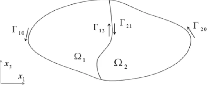
To illustrate this procedure, consider a two sub-region domain as showed in Figure 1. 111
Figure 1 A two sub-region domain
The boundary of Ω1 is divided into Γ10 and Γ12 – the latter is the contact line with
sub-112
region Ω2. Similarly, the boundary of Ω2is divided into Γ20 and Γ21. Considering each domain
separately, but taking a unique source point, it is possible to write one integral equation for 114
each domain, as: 115
c1ikui+∫
Γ10 p∗1
ikuidΓ10+∫ Γ12
p∗1
ikuidΓ12=∫ Γ10
u∗1
ikpidΓ10+∫ Γ12
u∗1
ikpidΓ12 (5)
116
c2ikui+∫
Γ20 p∗2
ikuidΓ20+∫ Γ21
p∗2
ikuidΓ21=∫ Γ20
u∗2
ikpidΓ20+∫ Γ21
u∗2
ikpidΓ21 (6)
For this hypothetical problem the sub-region Ω1is considered the standard domain. Although
117
this is an arbitrary choice, it is recommended that the standard sub-region should be chosen 118
as the predominant domain to improve the numerical accuracy. 119
Remembering the Kelvin fundamental solution for displacement, equation (2), and assum-120
ing the same Poisson ratio for both materials, the following relation can be written: 121
u∗1
ik =
G2 G1
u∗2
ik (7)
Also, with an equal Poisson ratio, the fundamental solution for tractionp*j becomes unique, 122
i.e. 123
p∗1
ik =p
∗2
ik =p
∗
ik (8)
At this moment, both equations are multiplied by the rate between the corresponding G
124
modulus per standard modulus, with no loss of validity. It is clear that for equation (5) there 125
is no difference because the rate is the unity. 126
Thus, multiplying both sides of equation (6) by G2/G1 and adding equation (5), the
fol-127
lowing expression can be written for the whole body: 128
c1
ikui+GG21c2ikui+(∫
Γ10 p∗
ikuidΓ10+ ∫ Γ20
G2
G1p
∗
ikuidΓ20)+
+(∫ Γ12
p∗
ikuidΓ12+ ∫ Γ21
G2
G1p
∗
ikuidΓ21)=(∫ Γ10
u∗1
ikpidΓ10+ ∫ Γ20
G2
G1u
∗2
ikpidΓ20)+
+(∫ Γ12
u∗1
ikpidΓ12+ ∫ Γ21
G2
G1u
∗2
ikpidΓ21)
(9)
On the right side of equation (9) it is possible to apply the relation given by (7) forward to 129
the integral over Γ20 and backward to the integral over Γ12. Then, organizing the terms, the
130
following expression is obtained: 131
(c1ik+G2
G1c 2
ik)ui+ ∫
Γ10 p∗
ikuidΓ10+ ∫ Γ12
p∗
ikuidΓ12+GG2 1(∫
Γ20 p∗
ikuidΓ20+ ∫ Γ21
p∗
ikuidΓ21)=
∫
Γ10 u∗1
ikpidΓ10+ ∫ Γ20
u∗1
ikpidΓ20+GG2 1(∫
Γ12 u∗2
ikpidΓ12+ ∫ Γ21
u∗2
ikpidΓ21)
Imposing the equilibrium condition on the last term of the right side of expression (10), the 132
term in parentheses becomes null, meaning that no traction approximation is performed for 133
the contact line reducing the number of degrees-of-freedom as desired. 134
The final integral equation for the heterogeneous domain without contact forces is given 135
by: 136
(c1
ik+ G2
G1c 2
ik)ui+ ∫
Γ10 p∗
ikuidΓ10+ ∫ Γ12
p∗
ikuidΓ12+
+G2
G1(∫ Γ20
p∗
ikuidΓ20+ ∫ Γ21
p∗
ikuidΓ21)= ∫ Γ10
u∗1
ikpidΓ10+ ∫ Γ20
u∗1
ikpidΓ20
(11)
Using a unique source point to derive equation (11) indicates that, when discretizing the whole 137
heterogeneous domain, each source point influences all boundary elements of the problem, 138
independently of which region it belongs to. 139
The illustrated example consists of only two different sub-regions, but the technique can 140
be applied to any number of sub-regions. Indeed, by the observation of expression (11), a 141
generalized equation can be written forns sub-regions: 142
{∑ns
m=1 Gm
G1
cmik}ui+ ns
∑
m=1
⎡⎢ ⎢⎢ ⎢⎢ ⎣
Gm
G1 ∫
Γm
p∗
ikuidΓm ⎤⎥ ⎥⎥ ⎥⎥ ⎦ = ne ∑
n=1
⎡⎢ ⎢⎢ ⎢⎢ ⎣Γ∫e
u1∗
ikpidΓe ⎤⎥ ⎥⎥ ⎥⎥ ⎦
(12)
where Γe is the external boundary and ne is the number of external surfaces. 143
For the algebraic procedure, the first thing to do is to define the predominant domain. For 144
the chosen region, the shear modulus shall be considered G1, and the other sub-regions may
145
be numbered from this one. 146
The systems of equations for all involved sub-regions are stored using all source points of 147
the original problem, even if the source point is not over the sub-region that is being inte-148
grated. Therefore, each sub-region system will have more rows than columns and each matrix 149
is multiplied by the shear modulus rate. Finally, superposition is assumed, adding each sub-150
regions matrix to the system of the predominant domain. Because the terms of the Gmatrix 151
(in each sub-region) related with contact interfaces were multiplied by the rate between differ-152
ent modulus, these terms become equal to the corresponding terms in the standard equation 153
system. After applying the equilibrium condition of contact traction, the sum of those terms 154
becomes null, algebraically eliminating all contact tractions. The technique is applicable to 155
both layered sub-regions and internal inclusions. 156
The singularity of the H matrix can still be calculated using the rigid body concept, by 157
the sum of odd and even terms of each row for each sub-region separately. For the Gmatrix, 158
singularity is solved by a subtraction technique, as already mentioned in the previous section. 159
For internal points, as the original system is multiplied by the shear modulus rate, it is 160
necessary to correct the displacement multiplying it by the inverse rate at the end of the 161
numerical solution. 162
It is also possible to calculate stresses at internal points, using the Hooke constitutive law 163
collocation points: 165
σjik=−
ns
∑
m=1 Gm
Gj Γ∫ j
S∗m
ikjumi dΓ+∫
Γe D∗
ikjpidΓe (13)
where Sikj* and Dikj* are well-known tensors for the stress equation [3]. 166
2.2 Internal Load Lines
167
Some engineering problems require modeling load lines inside bodies. That is the case of piles 168
analysis in foundation engineering problems, in which the piles inserted in the soil can be 169
modeled via FEM and act as internal load lines on BEM meshes [20]. 170
For this type of analysis, there must be load line elements implemented in BEM formulation. 171
However, load lines do not form closed regions and must be completely inside the body domain. 172
Double nodes are used in the points where load lines meet the boundary elements, avoiding 173
the continuity of distributed forces values with different meanings (shear and normal) over each 174
element. 175
Regarding tractions, load lines work exactly as boundary elements, i.e., source points inte-176
grate tractions weighted by fundamental displacements generating new columns in Gmatrix. 177
However, as displacements are not approximated over load lines, no new column is generated in 178
Hmatrix. Displacements at internal points are usually calculated as post processing, because 179
the solution of the problem is only dependent on boundary values. However, when piles are con-180
nected to solids, the contact forces (tractions at load lines) are functions of pile displacements; 181
therefore the displacements of load line nodes are directly written in the system of equations 182
introducing source points geometrically coincident with those nodes. This procedure results in 183
additional lines in matrix Hincluding non-zero values related to boundary displacements and 184
diagonal unit values related to domain displacements. For G matrix non-zero values appear 185
for boundary and load lines columns, see equation (14). The weak singularities present in G 186
matrix calculations are treated following the same procedure used for boundary elements. The 187
final algebraic system is written as: 188
[ Hee 0
Hie I ]
⋅{ Ue Ui }
=[ Gee Gei
Gie Gii ]
⋅{ Pe Pi }
(14)
where index e identifies boundary terms, index i indicates internal nodes of load lines and I
189
is the identity matrix. 190
The same shape functions can be adopted for the load line description as boundary ele-191
ments, using Lagrange polynomials, see appendix A. These polynomials allow the use of curved 192
internal load lines of any load order. Another advantage of load lines is that they may have 193
any direction, making it possible to analyze inclined piles. 194
As for heterogeneous domains the integration procedure is affected only by the fundamental 195
values, and the consideration of load lines trespassing regions is straightforward. First, one 196
must identify the sub-region each load line is inserted in. Then, during the matrices storage 197
One considers a load line trespassing two regions by dividing it into two elements, each one 199
inserted in a different domain. Superposition is still valid, and the final system includes all 200
load lines. 201
3 FEM PROCEDURE
202
The frame structure is modeled adopting the Finite Element Method. Using the positional 203
formulation and an intermediate non-dimensional space it is possible to apply a simple La-204
grangean formulation for the consideration of geometric nonlinearity with exact kinematics. 205
The same formulation is used in [13] for the analysis of 2D frames, assuming a nonlinear and 206
objective engineering strain measurement for the kinematics assumption. The authors also 207
present a comparison between Reissner and Euler-Bernoulli kinematics, checking the influence 208
of shear deformation on bending problems. 209
The accuracy of positional FEM formulation has also been proved by [7, 8, 14]. 210
In the present study, the Green strain tensor and second Piola-Kirchhoff stress are adopted. 211
Both of them, as well as the energy functional are written as functions of the structures position. 212
To find the equilibrium configuration, the minimum total potential energy principle is used 213
regarding nodal position parameters. 214
As one can see, the FEM formulation adopted here consists basically in assuming the 215
position of the structure as the main variable of the problem, instead of displacements. In 216
this study, node and angular positions are assumed as the variables for each node in the finite 217
element mesh. 218
3.1 Kinematics
219
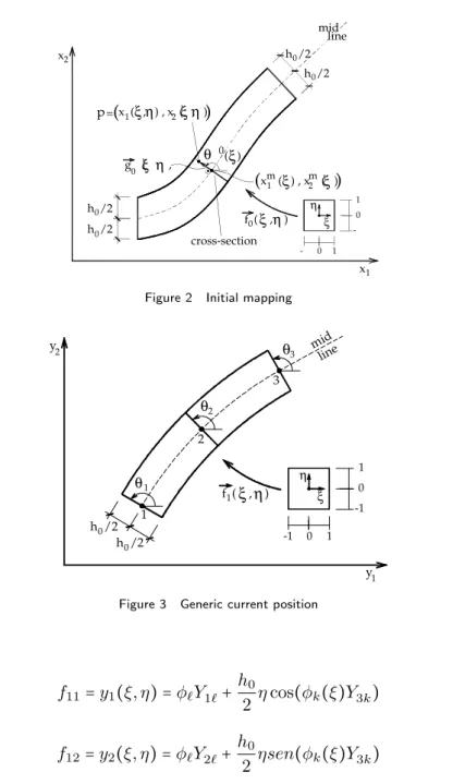
Figure 2 presents the mapping from a non dimensional space to the initial configuration of 220
a generic bar. This mapping is performed by Lagrange shape functions of any order (see 221
appendix) and nodal initial positions or coordinates. The nodal initial angle indicates an 222
orthogonal direction with respect to the mid line of the element. Functionf⃗0(ξ, η)is a mapping
223
that locates any point inside the initial domain from a point in the non-dimensional domain. 224
Figure 3 is a similar drawing of a generic current position of the bar. In this case the 225
angular positions do not indicate an orthogonal direction to the reference line, but a direction 226
that composes both bending and shear contributions to the cross-section position. In the same 227
way, function f⃗1(ξ, η) is the mapping from the non-dimensional space to the current position.
228
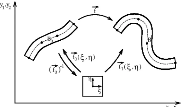
Putting both mappings together, Figure 4 presents the desired mapping, i.e., from the 229
initial to the current configuration. 230
The initial and current mappings are written for each coordinate as: 231
f01=x1(ξ, η)=ϕℓX1ℓ+
h0
2 ηcos(ϕk(ξ)θ
0
k) (15)
232
f02=x2(ξ, η)=ϕℓX2ℓ+
h0
2 ηsen(ϕk(ξ)θ
0
1
x x2
0
h /2
h /20
h /2 h /20 0
line mid
cross-section
0
g ( , ξ η θ
0 ( )ξ
x ( ) , x ( )m1 ξ 2mξ
2ξ η ξ η 1
x ( , ) , x ( , )
p=( )
ξ
η 1
0
-0 1 -ξ f ( , )0 η
) (
Figure 2 Initial mapping
1
0 0
h /2 h /2
0 -1
η ξ
ξ 1
f ( , )η
1
y1 0 -1 y2
1
θ
1
2
θ
2
θ
3
3
mid line
Figure 3 Generic current position
233
f11=y1(ξ, η)=ϕℓY1ℓ+ h0
2 ηcos(ϕk(ξ)Y3k) (17) 234
f12=y2(ξ, η)=ϕℓY2ℓ+ h0
2 ηsen(ϕk(ξ)Y3k) (18)
where x and y stand for initial and current positions, respectively, ℓ represents node and 235
the corresponding shape function ϕℓ,Xiℓ and Yiℓ are the initial and current nodal positions, 236
respectively, and θ0ℓ and Y3ℓ=θℓ are initial and current nodal angular positions. Defining the
237
current angular position as Y3ℓ=θℓ is useful to generalize the FEM solution procedure in the 238
next section. 239
One may write the total mapping or the change of configuration function as: 240
⃗
f =f⃗1○( ⃗f0) −1
B
1 2
x ,x y ,y1 2
f
0 B
0
f ( , )ξ η
η f ( , )1 ξ f 0
( )-1
η ξ
Figure 4 Positional mapping from initial to current position
However, only its gradient is necessary to develop the proposed formulation, i.e.: 241
A=A1.(A0)−1 (20)
where the dot indicates a simple contraction, A1
is the gradient of the current mappingf⃗1(ξ, η)
242
and A0
is the gradient of the initial mapping f⃗0(ξ, η). These gradients are written as:
243
A0=⎡⎢⎢⎢
⎢⎣ ∂f10
∂ξ ∂f10
∂η ∂f0 2 ∂ξ ∂f0 2 ∂η ⎤⎥ ⎥⎥ ⎥⎦= ⎡⎢ ⎢⎢ ⎢⎣ ∂x1 ∂ξ ∂x1 ∂η ∂x2 ∂ξ ∂x2 ∂η ⎤⎥ ⎥⎥ ⎥⎦ (21) 244
A1=⎡⎢⎢⎢
⎢⎣ ∂f1 1 ∂ξ ∂f1 1 ∂η ∂f1 2 ∂ξ ∂f1 2 ∂η ⎤⎥ ⎥⎥ ⎥⎦= ⎡⎢ ⎢⎢ ⎢⎣ ∂y1 ∂ξ ∂y1 ∂η ∂y2 ∂ξ ∂y2 ∂η ⎤⎥ ⎥⎥ ⎥⎦ (22)
In order to achieve the Green strain tensor one calculates the right Cauchy-Green stretch 245
tensor Cof the change of configuration function as: 246
C=At.A=(A0)
−t
.A1t.A1.(A0)−1 (23)
and the Green strain, assumed in this study as the strain measurement, is given by: 247
E=1
2(C−I) (24)
3.2 Potential energy minimization - equilibrium
248
As previously mentioned, the total mechanical energy should be minimized in order to solve the 249
problem. The simple specific strain energy assumed is the so-called Saint-Venant-Kirchhoff, 250
written in a simplified form for the analyzed problem as: 251
ue= E 2 {(E
2
11+E
2
22)+(E
2
12+E
2
21)} (25)
Therefore, the total potential energy for a conservative elastic structure is given by: 253
Π=Ue+P (26)
where Ue is the elastic strain energy and P the potential energy of applied forces. 254
A Lagrangian description is assumed by writing the strain energy over the initial volume 255
as follows: 256
Ue=∫ V0
uedV0 (27)
The potential energy of applied forces (concentrated and conservative) is written as: 257
P =−F.Y (28)
As the Green strain is a function of nodal current positions (positional parameters), the 258
same is stated forUe andP.Applying the minimum total potential energy principle regarding 259
positionsY follows the non-linear equilibrium equation: 260
∂Π
∂Y =∫
V0 ∂ue
∂YdV0−F =Fint−F =g (29)
Note that the integral over the initial volume of ∂ue/∂Y(for an arbitrary position) is also 261
understood as the internal forces Fint. Thus, g is a vector that assumes null value when the 262
solution is obtained, i.e., when the equilibrium position of the structure is verified. However, 263
it is understood as the unbalanced force of the mechanical system when a trial position is 264
assumed. 265
For the numerical solution the Newton-Raphson procedure is used. In order to do that, a 266
Taylor expansion from an initial trial solutionYarb of g is carried out as follows: 267
g(Y)=g(Yarb)+ ∇g(Yarb).∆Y +Θ 2
=0 (30)
Neglecting higher-order terms (Θ2
) and reorganizing the other terms, equation (30) can be 268
rewritten to provide the following expression: 269
∆Y =−(∇g(Yarb))−1g(Yarb)=K−1
T .(F−Fint(Yarb)) (31)
whereKT is the hessian matrix or the tangent stiffness matrix, given by the second derivative 270
of the strain energy. 271
The solution is achieved by assuming an arbitrary position Yarb to calculate the internal 272
forces Fintand the hessian matrix KT. For the very first iteration the initial configuration X 273
is taken asYarb. 274
The correction position vector ∆Y is found by equation (31) and used to “correct” the 275
arbitrary solution as follows: 276
Yarb+1=Yarb+∆Y (32)
This new arbitrary position is assumed as the current configuration and the iterative process 277
is carried out until ∣∆Y∣ becomes smaller than a tolerance value. With both FEM and BEM 278
computational codes prepared, the numerical coupling is performed for the fulfillment of this 279
4 BEM-FEM COUPLING
281
The numerical coupling is performed following the idea of inserting BEM’s conditions in the 282
finite element mesh by condensing the BEM algebraic system regarding coupled nodes. To do 283
so, it is necessary to identify the coupled elements in each BEM and FEM mesh. 284
For the boundary element domain the following algebraic system is written: 285
[ Hcc Hcl
Hlc Hll ] {
UB c
UB l
}=[ Gcc Gcl
Glc Gll ] {
PB c
PB l
} (33)
where c is the index to identify the coupled terms and l is used for the free terms (those not 286
coupled to the finite element mesh). The superior index B shows that those terms are related 287
to the BEM formulation. U is a vector containing the nodal displacements and P another 288
vector for distributed forces. 289
On the other hand, the finite element structure mesh is given by the algebraic system 290
written in a simplified form as: 291
[ Kcc Kcm
Kmc Kmm ] {
UcF UF
m }
={ F
F c
FF m }
(34)
Again, cis related to the coupled terms. The superior indexF is related to FEM formula-292
tion, and index m is used to identify the nodes which are not coupled to the boundary mesh. 293
Vector F represents concentrated nodal forces vector. In particular UF is related to ∆Y in 294
the iterative procedure, as a change in position is in fact a displacement. 295
From (33) it is possible to write two equations. Isolating Ul and organizing the result, we 296
obtain the following expression: 297
¯
HccUcB=G¯ccPcB+T (35)
where: 298
¯
Hcc=[Hcc−HclH
−1
ll Hlc] (36)
¯
Gcc=[Gcc−HclH
−1
ll Glc] (37)
T =[Gcl−HclH
−1
ll Gll]PlB (38)
Pre-multiplying both sides of (35) by aQcmatrix, which is originated from shape functions 299
integration on the finite element mesh, the result does not change. The objective ofQc matrix 300
is to convert distributed forcesP into concentrated forces F: 301
QcP =F (39)
In this way it is possible to transform the boundary distributed forces into FEM nodal forces 302
to be applied on FEM nodes. As a result of this multiplication, expression (35) becomes: 303
¯
where: 304
¯
Kcc=QcG¯
−1
ccH¯cc (41)
305
¯
Pc=QcG¯
−1
ccT (42)
306
FcB =QcPB
c (43)
From (40) it is possible to isolate the equivalent applied concentrated forces from boundary 307
elementsFcB. 308
Over the interface line the following compatibility and equilibrium conditions must be 309
imposed: 310
UcB =UF
c (44)
311
FcB =−FcF (45)
Back to the FEM algebraic system and applying conditions (44) and (45), a final algebraic 312
system is obtained for the coupled structure: 313
[ (Kcc+K¯cc) Kcm
Kmc Kmm ] {
UcF UmF }={
¯
Pc
FmF } (46)
This algebraic system represents the frame structure coupled to the heterogeneous soil 314
domain. The ¯Kcc matrix is understood as an equivalent soil’s stiffness matrix condensed on 315
contact nodes. Its physical significance is that soil’s conditions computed in BEM model are 316
added to the frame structure modeled by FEM as “springs”. However, these “springs” have a 317
more refined concept as they consider the soil’s continuity and every condition from the BEM 318
model, unlike Winklers approximation. 319
At each iteration, it is necessary to correct the internal force vector of the frame structure by 320
adding the reaction values from soil restriction. Vector ¯Pchas these load conditions on interface 321
lines and will update theFF
c vector at each iteration of the Newton-Raphson procedure. 322
As the soil is assumed here linear elastic, the equivalent stiffness matrix is calculated only 323
once at the very first iteration of the nonlinear analysis. 324
The solid heterogeneous model is still valid, as the alternative sub-region technique is 325
performed before the condensation of BEM algebraic system to the BEM-FEM interface. 326
It is important to observe that BEM formulation does not consider rotation a degree-of-327
freedom. Therefore, to perform the numerical coupling, null rows and columns were inserted 328
in the BEM matrices. 329
Various numerical examples were processed and compared to analytical solutions or results 330
obtained from FEM commercial software. Some of these examples are showed in the next 331
5 EXAMPLES
333
5.1 Tensile bar
334
This is a simple example of a straight bar under a tensile force. It is presented here to prove 335
the formulation efficiency, as the result can be compared to the analytical solution. 336
Half of the bar is modeled via BEM and the other half via FEM, with a coupled interface 337
in the middle section, as shown in Figure 5. The section area is unitary as a unitary width is 338
adopted. 339
Figure 5 BEM-FEM model for straight tensile bar
The boundary mesh is divided into three domains to test the alternative technique of sub-340
regions. The material properties are the same for all elements, on both BEM and FEM meshes 341
(E1= E2= E3= Ebar =10000kN/cm 2
). The finite element coupled to the boundary element 342
has thickness of 20 cm (more rigid) to allow the comparison with the analytical result. The 343
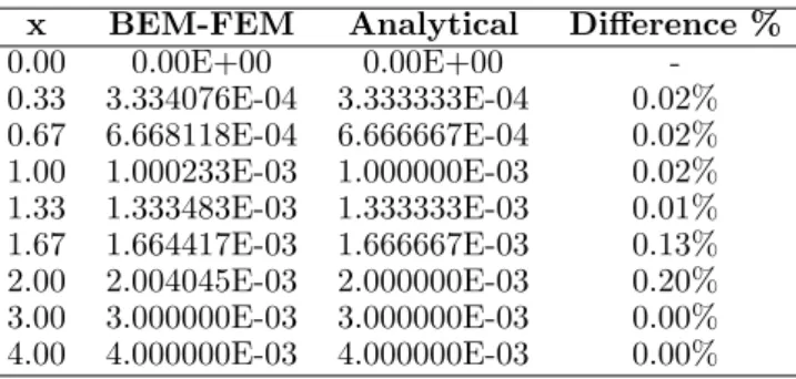
analytical solution is given by: 344
u(x)= F
EAx (47)
The results are shown in Table 1. 345
Table 1 −Horizontal displacement (cm) along the bar length
x BEM-FEM Analytical Difference %
0.00 0.00E+00 0.00E+00
-0.33 3.334076E-04 3.333333E-04 0.02% 0.67 6.668118E-04 6.666667E-04 0.02% 1.00 1.000233E-03 1.000000E-03 0.02% 1.33 1.333483E-03 1.333333E-03 0.01% 1.67 1.664417E-03 1.666667E-03 0.13% 2.00 2.004045E-03 2.000000E-03 0.20% 3.00 3.000000E-03 3.000000E-03 0.00% 4.00 4.000000E-03 4.000000E-03 0.00%
As one can see, the connecting element flexibility allows a small difference along the central 346
5.2 Vertical pile in homogeneous domain
348
This is an example of a vertical pile structure inserted in a homogeneous domain and subjected 349
to a bending moment, as it is shown in Figure 6. 350
Figure 6 Vertical pile in homogeneous domain
The continuum domains Young modulus is Es=21000 kPawhile the pile structure’s mod-351
ulus isEp= 21 GP a. The Poisson ratio is taken asν =0.2 for both soil and pile materials. A 352
unitary influence width for the soil domain is considered and the plane stress is assumed. The 353
pile has a circular section area with diameter D= 30 cm, resulting in a 706.8 cm2 area and
354
inertia moment of 39760cm4
. The pile has a small length of 2.0 cm outside of soil domain on 355
which the concentrated load is applied. A quadratic approximation is adopted for both finite 356
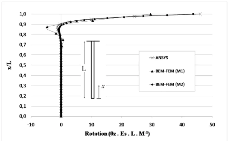
and boundary elements. Two regular meshes (varying the piles discretization) are used: M1 357
is a mesh formed by 24 boundary elements (each element has a length of 5.0 m), and 8 finite 358
elements (element length of 2.5 m) along the piles height; for mesh M2 50 finite elements are 359
considered for the piles discretization (element length of 0.4 m). 360
The results were compared to the same example processed with the commercial ANSYS® 361
software. For the ANSYS® model a mesh with 3200 plane stress elements was used for 362
continuum domain’s discretization and 43 conventional beam elements for the frame’s mesh. 363
The results for horizontal displacement and section rotation are presented in Figures 7 and 8. 364
Distributed forces along the piles length are also compared, as shown in Figure 9. The 365
distributed force is directly obtained from the developed program. For ANSYS®, these values 366
are obtained dividing the nodal reaction by each finite element length. 367
As one can see, the results compare very well despite the difference of the adopted formu-368
lations. 369
5.3 Pile inclined in a layered soil
370
An inclined pile foundation structure subjected to vertical and horizontal concentrated forces 371
is now considered inserted in a layered soil, as shown in Figure 10. 372
The frame structure has a rectangular section of10x15 cm resulting in a150 cm2
Figure 7 Horizontal displacement along the piles height
Figure 8 Rotation of sections along the piles height
inertia moment of 2812.5 cm4
. The Young modulus is Ep = 2100 MPa and Poisson ratio is 374
null. For the soil, the elastic modulus of each layer is shown in Figure 10 and a unitary width 375
of influence is considered. 376
Two regular meshes (with quadratic elements) are used: M1 is a mesh formed by 20 377
boundary elements and 4 finite elements along the piles height, with elements length varying 378
from 1.0 m to 2.75 m; M2 has 210 boundary elements for the soil and 40 finite elements for 379
the piles discretization (each element has a length of 0.1 m). 380
The results are again compared to ANSYS® model, with 3750 plane strain elements for 381
the soil’s mesh and 41 conventional beams elements for the pile. 382
For this analysis, forces FH and FV were separately applied and their values are FH = 10 383
kN and FV = -50 kN. The pile has a small length of 2.0 cm outside of soil domain on which
384
the concentrated load is applied. 385
Figure 9 Horizontal distributed force along the piles height
Figure 10 Pile inclined in heterogeneous soil
12 exhibits the vertical displacement caused by FV. 387
There are no significant differences among the results obtained with meshes M1 and M2, 388
which demonstrate the numerical convergence for this problem. 389
5.4 Bending frame
390
This is an example of the applicability of the proposed technique. It consists of a slender 391
frame structure coupled to a heterogeneous soil. In this case, geometric nonlinear analysis is 392
required to determine the structure’s displacement with better accuracy. To demonstrate the 393
importance of considering the soil-structure interaction, the results are compared to the same 394
frame fixed by a rigid support instead of soil’s domain for the contact nodes. Geometrical 395
linear and nonlinear analyses are performed and compared. 396
Figure 13 presents the soil and frame dimensions and other information of interest. 397
Figure 11 Horizontal displacement along the piles height caused byFH
Figure 12 Vertical displacement along the piles height caused by FV
section area of0.1164 m2
and inertial moment of0.0183 m4
. The Young modulus isE = 210
399
GPa. A cubic approximation is adopted for both BEM and FEM models. Two regular meshes 400
are used, varying the discretization of the frames length inside the soil’s domain: M1 is a mesh 401
formed by 14 boundary elements and 2 finite elements along the inserted length (each finite 402
element has a length of 7.5 m); for mesh M2 6 finite elements are considered for the inserted 403
length, and in this case, each element has a length of 2.5 m. 404
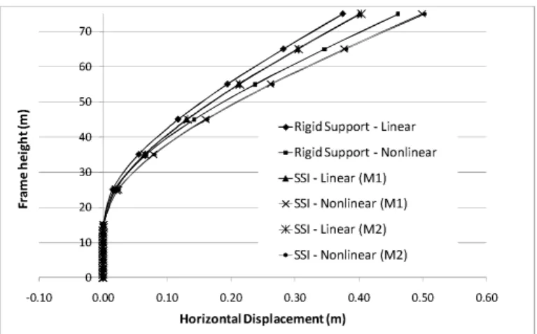
The results for horizontal displacement considering linear and nonlinear analyses for the 405
fixed support model and soil-structure interaction (SSI) model are presented in Figure 14. 406
Note that an additional horizontal displacement is verified by considering the soil-structure 407
interaction (SSI), as the soil’s deformability influences the final results. 408
Table 2 shows the comparison of the maximum horizontal displacement at the top of the 409
frame structure for linear and nonlinear analyses, for both the rigid support and soil-structure 410
Figure 13 Slender bending frame supported by a layered soil
0 10 20 30 40 50 60 70
-0.10 0.00 0.10 0.20 0.30 0.40 0.50 0.60
Fr am e he ig ht (m )
Horizontal Displacement (m) Rigid Support - Linear Rigid Support - Nonlinear SSI - Linear (M1) SSI - Nonlinear (M1) SSI - Linear (M2) SSI - Nonlinear (M2)
Figure 14 Horizontal displacement along the frames height
The difference between a linear analysis with rigid support and the nonlinear analysis 412
considering soil-structure interaction is 34%, which proves that the simplified model may not 413
be appropriate in this case. 414
The consideration of soil-structure interaction also leads to a different distribution the 415
internal efforts on the frame structure model. It is interesting to measure here the influences 416
that these differences may cause on the structural design for a safer and more economical 417
project. 418
The internal normal force, shear and bending moment along the frame’s height are pre-419
sented next. 420
Also, the frames influence over the soil contact interface can be introduced into the BEM 421
program to compute the soil final displacements and stresses. It is possible to determine the 422
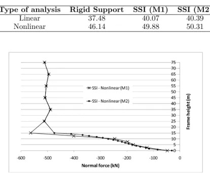
Table 2 Maximum horizontal displacement (cm) at the top of the structure
Type of analysis Rigid Support SSI (M1) SSI (M2)
Linear 37.48 40.07 40.39
Nonlinear 46.14 49.88 50.31
0 5 10 15 20 25 30 35 40 45 50 55 60 65 70 75
-600 -500 -400 -300 -200 -100 0
Fr am e he ig ht (m )
Normal force (kN)
SSI - Nonlinear (M1)
SSI - Nonlinear (M2)
Figure 15 Normal force along the frames height
6 CONCLUSIONS
424
The alternative technique for sub-regions on BEM has been successfully applied allowing for 425
the consideration of multiple inclusions. The strategy reduces the number of variables as 426
it eliminates the traction approximation on contact interfaces. It is possible to consider a 427
large number of sub-regions in a much simpler way than by using the classical sub-region 428
technique. The final matrix is compact and full. Load lines are also implemented allowing for 429
the simulation of internal elements in any direction and passing through different domains. 430
The FEM based on positions is used to implement a Lagrangean formulation considering the 431
frame geometric nonlinear behavior with exact kinematics. 432
The developed BEM-FEM coupling introduces the linear soil influence into the frame non-433
linear system of equations. The main advantage of the procedure is the calculation of the 434
matrix soil influence only once in a very compact way, reducing the amount of calculations in 435
the iterative solution process. 436
The coupling strategy is more powerful than the usual Winkler procedure as it takes into 437
account the influence of different foundations, or even buildings, on each other. Moreover the 438
use of BEM is much more economical than the use of FEM to model the soil. Examples show 439
the good behavior of the procedure when compared to a generalist commercial package, as 440
ANSYS® for instance. 441
Moreover, this study has emphasized the importance of the influence of the soil’s flexibil-442
ity on the nonlinear behavior of structures. It is important to mention the two-dimensional 443
0 5 10 15 20 25 30 35 40 45 50 55 60 65 70 75
-400 -200 0 200 400 600 800
Fr am e he ig ht (m )
Shear force (kN)
SSI - Nonlinear (M1)
SSI - Nonlinear (M2)
Figure 16 Shear force along the frames height
0 5 10 15 20 25 30 35 40 45 50 55 60 65 70 75
-2.000 -1.500 -1.000 -500 0 500
Fr am e he ig ht (m )
Bending Moment (kN.m)
SSI - Nonlinear (M1)
SSI - Nonlinear (M2)
Figure 17 Bending moment along the frames height
arbitrarily. In the future this formulation should be extended for 3D representation in order 445
to provide more generality to the proposed methodology. 446
APPENDIX A – HIGH-ORDER ELEMENTS WITH LAGRANGE POLYNOMIALS
447
Both BEM and FEM formulation are implemented with high-order elements, assuming La-448
grange polynomials for shape functions description. The Lagrange polynomials are given as 449
follows: 450
ϕl= n
∏
i≠k
i=1
(ξ−ξi
ξk−ξi)
(48)
0 5 10 15 20 25 30 35 40 45 50 55 60 0
5 10 15 20 25 30 35 40 45
-0.00065 -0.0006 -0.00055 -0.0005 -0.00045 -0.0004 -0.00035 -0.0003 -0.00025 -0.0002 -0.00015 -0.0001 -5E-005 0 5E-005
00 5 10 15 20 25 30 35 40 45 50 55 60
5 10 15 20 25 30 35 40 45
-44 -40 -36 -32 -28 -24 -20 -16 -12 -8 -4 0 4 8 12
Figure 18 (a) Soil deformation in meters and (b) vertical stress component in kPa
assume values from -1 to +1 on dimensionless space. Therefore, it is possible to define any 452
point of the element from its ξ coordinates. 453
A numerical subroutine based on equation (48) is implemented in both BEM and FEM 454
computational codes to generate all shape functions of discrete elements. The user must only 455
introduce the desired order for the discrete elements and the number of points for Gaussian 456
quadrature. 457
Figure 19 Curved element in dimensionless coordinates
References
458
[1] M.H. ALIABADI. The boundary element method. Applications in solids and structures. J. Wiley, Chichester, New
459
York, 2002.
460
[2] J. BONET. Finite element analysis of air supported membrane structures. Comput. Methods Appl. Mech. Eng,
461
190:579–595, 2000.
462
[3] C.A. BREBBIA and J. DOMINGUEZ. Boundary elements: and introductory course. Computational Mechanics
463
Publications, London, 1992.
464
[4] C.A. BREBBIA, J.C.F. TELLES, and L.C. WROBEL. Boundary Element Techniques. Springer Verlag, Berlin,
465
1984.
466
[5] H.B. CODA. Contribui¸c˜aoo `a an´alise dinˆamica transiente de meios cont´ınuos pelo m´etodo dos elementos de contorno.
467
tese (livre docˆencia), 2000.
468
[6] H.B. CODA. An exact FEM geometric non-linear analysis of frames based on position description. In: XVIII.
469
Congresso Brasileiro De Engenharia Mecˆanica, S˜ao Paulo, 2003.
470
[7] H.B. CODA. Two dimensional analysis of inflatable structures by the positional fem. Latin American Journal of
471
Solids and Structures, 6:187–212, 2009.
[8] H.B. CODA and M. GRECO. A simple fem formulation for large deflection 2d frame analysis based on position
473
description. Computer Methods in Applied Mechanics and Engineering, 193:3541–3557, 2004.
474
[9] H.El. GANAINY and M.H.El. NAGGAR. Efficient 3d nonlinear winkler model for shallow foundations.Soil Dynamics
475
and Earthquake Engineering, 29(8):1236–1248, 2009.
476
[10] H.SCHOLZ. Approximate p-delta method for sway frames with semi-rigid connections.J. Construct. Steel Research,
477
15:215–231, 1990.
478
[11] A. K. L. KZAM. Formula¸c˜ao dual em mecˆanica da fratura utilizando elementos de contorno curvos de ordem qualquer.
479
disserta¸c˜ao (mestrado), 2009.
480
[12] J.C. LACHAT. Effective numerical treatment of boundary-integral equations: A formulation for three-dimensional
481
elastostatics.Int. J. Numer. Methods Eng, 10:991–1005, 1976.
482
[13] MACIEL, Daniel Nelson, and H.B. CODA. Positional finite element methodology for geometrically nonlinear analisys
483
of 2d frames. Revista Minerva, 5:73–83, 2008.
484
[14] R. L. MINSKI. Aprimoramento de formula¸c˜ao de identifica¸c˜ao e solu¸c˜ao do impacto bidimensional entre estrutura e
485
anteparo r´ıgido. disserta¸c˜ao (mestrado), 2008.
486
[15] J.B. PAIVA and M.H. ALIABADI. Boundary element analysis of zoned plates in bending.Comput Mech, 25:560–6,
487
2000.
488
[16] J.B. PAIVA and M.H. ALIABADI. Bending moments at interfaces of thin zoned plates with discrete thickness by
489
the boundary element method. Eng Anal Boundary Elem, 28:747–51, 2004.
490
[17] D.B. RIBEIRO and J.B. Paiva. An alternative multi-region bem technique for three-dimensional elastic problems.
491
Engineering Analysis with Boundary Elements, 33:499–507, 2009.
492
[18] R.A. SOUZA and J.H.C. REIS. Intera¸c˜ao solo-estrutura para edifcios sobre funda¸c˜oes rasas. Acta Sci. Technol.,
493
Maring´a, 30(2):161–171, 2008.
494
[19] W.S. VENTURINI. Boundary Element Method In Geomechanics. Springer-Verlac, Berlin, 1984.
495
[20] W.S. VENTURINI. Um estudo sobre o m´etodo dos elementos de contorno e suas aplica¸c˜oes em problemas de
496
engenharia. tese (livre docˆencia), 1988.
497
[21] W.S. VENTURINI. Alternative formulations of the boundary element method for potential and elastic problems.
498
Engineering Analysis with Boundary Elements, 9:203–207, 1992.