Study of EEG spectral bands from Parkinson's disease patients treated with transcranial magnetic stimulation

STUDY OF EEG SPECTRAL BANDS FROM PARKINSON’S

DISEASE PATIENTS TREATED WITH TRANSCRANIAL

MAGNETIC STIMULATION

By

Cristiana Margarida Alão Ferreira

STUDY OF EEG SPECTRAL BANDS FROM PARKINSON’S

DISEASE PATIENTS TREATED WITH TRANSCRANIAL

MAGNETIC STIMULATION

Thesis presented to Escola Superior de Biotecnologia of the Universidade

Católica Portuguesa to fulfill the requirements of Master of Science degree in

Biomedical Engineering.

by

Cristiana Margarida Alão Ferreira

Place: Tampere University of Technology

Resumo

A doença de Parkinson é uma condição degenerativa do Sistema Nervoso Central, relacionado com a perda de um neurotransmissor, a Dopamina. Os principais sintomas presentes são: os tremores nos membros assim como, o maxilar e a face; a instabilidade postural e a afectação do equilíbrio e coordenação. Em Portugal a doença de Parkinson afecta cerca de vinte mil de pessoas, enquanto na Finlândia são cerca de dez mil pessoas. Estes doentes são normalmente sujeitos a medicações que reduzem parte dos sintomas, como o caso da Levodopa (L-dopa), e também é comum estes doentes apresentarem problemas na marcha.

Com este estudo é pretendido ver se a técnica Estimulação Magnética Transcraniana pode ser um tratamento alternativo para os doentes de Parkinson. Estas pessoas detêm uma actividade da banda de frequência Beta superior ao normal, e pretende-se que esta diminua após o tratamento. Para tal foram adquiridos dados de electroencefalograma (EEG) de 26 pacientes previamente divididos em dois grupos, um dos quais receberia a estimulação e o outro seria o seu controlo. Este estudo baseia-se num protocolo duplamente cego, onde os pacientes foram distribuídos aleatoriamente, e nem os médicos ou técnicos têm conhecimento dos grupos. Os doentes de Parkinson seleccionados tinham idades compreendidas entre 40-80 anos, classificados de acordo com os parâmetros de UK-PD-Brain-Bank-criteria Hoehn

–Yahr-stage (escala: 2-4), eram medicados com 300mg ou mais de Levodopa ou semelhante; e

apresentavam dificuldades no andar (demorando 6 segundos ou mais a percorrer 10 metros). A técnica intermittent Theta Burst Stimulation (iTBS) foi aplicada no Córtex Motor e no Córtex Dorsolateral Prefrontal (DLPFC) dos pacientes pertencentes ao grupo experimental.

Como tratamento dos dados de EEG foi usada a Análise de Componentes Independentes, assim como Fast Fourier Transform para o cálculo da Potência no domínio das frequências. No entanto a hipótese não foi confirmada, uma vez que os resultados obtidos não mostraram as diferenças significativas desejadas entre o grupo controlo e o grupo que sofreu a estimulação no que concerne a actividade da frequência Beta.

Abstract

Parkinson’s disease (PD) is a degenerative condition of the Central Nervous System, that is related with the loss of the neurotransmitter, Dopamine. The main symptoms are: tremors especially on limbs, jaw and face; the postural instability and loss of control of coordination and balance. In Portugal there are twenty thousand people that suffer from Parkinson’s disease, and ten thousand in Finland. Usually these people take medication to reduce the symptoms, such as Levodopa (L-dopa) and they also have problems walking.

The study intended to verify if the technique Transcranial Magnetic Stimulation (TMS) may be an alternative treatment for Parkinson's disease patients. These patients have the activity of beta band higher than normal, and it is supposed to be lower after treatment. For that, electroencephalogram (EEG) data of 26 patients were acquired and divided into two groups: one that would receive the stimulation and the other would be its control. The study was designed to be a random, double-blind study. The PD patients included 40-80 years old, were classified according to UK-PD-Brain-Bank-criteria, Hoehn-Yahr-stage 2 to 4; also, these patients were medicated with a total dose of Levodopa or other Dopamine agonist agents of equal or more than 300 mg or more revealed problems with walking (taking 6 or more seconds to walk a 10 meter distance). Standard tests were performed before and during this study, to test walking capacity of patients. The intermittent Theta Burst Stimulation (iTBS) was applied to the Motor Cortex and Dorsolateral Prefrontal Cortex (DLPFC) of patients belonging to the experimental group.

While processing the EEG data, the Independent Component Analysis (ICA), as well as Fast Fourier Transform (FFT) were used to calculate the band power in the frequency domain. However the hypothesis was not fully confirmed, since the results showed no significant differences between the sham group and the group that received stimulation as for the activity of Beta band was concerned.

Acknowledgment

I

Also would like to thank to all my teachers, especially to my course coordinator João Paulo Ferreira for his availability and knowledge.

Finally, thanks to my family and friends who supported me in any respect, along this journey.

Contents

1.Introduction………..1

1.1.Parkinson disease………1

1.1.1.Background………..………..…….2

1.1.2.Treatment………..……….……...4

1.2.Anatomy and Physiology of the Motor Cortex……….……6

1.2.1.Primary Motor Cortex (M1)………..……….……6

1.2.2.Premotor Area………..……….……...7

1.2.3.Supplementary Motor Area………..……….7

1.3.Electroencephalogram (EEG)………8

1.3.1.Electrode Location Systems………..…….……..8

1.3.2.EEG signal – Frequency Bands………..………..11

1.3.3.Artifacts present in the Electroencephalogram………..………….12

1.4.Transcranial Magnetic Stimulation………..15

1.4.1.Single, Paired and Repetitive variants of Transcranial Magnetic Stimulation………...16

1.4.2.Types of coil………..………18

2.State of art……….21

2.1.Objectives of the Study……….………22

3.Materials and Methods………23

3.1.Preprocessing data………24

3.2.Independent Component Analysis………..24

3.3.Time Frequency Analysis……….27

3.4.Statistical Methods……….………...28

4.Results and Discussion………...31

5.Conclusions and Recommendations……….45

6.References………47

List of figures

Figure 1.1.1.1 – Illustration of the interaction of neurotransmitters in the synaptic

cleft………3

Figure 1.1.2.1 – Deep Brain Stimulation schematic figure and Implantable Pulse Generator.………4

Figure 1.2.1 – Segmentation of the brain, location of the Motor Cortex. Also can be seen the Primary Motor Cortex, Premotor Area and Supplementary Area……….……..6

Figure 1.3.1 – Example of electroencephalogram (EEG), electrooculargram (EOG) and electromyogram (EMG) ……….………8

Figure 1.3.1.1 – Electrodes distribution through the scalp, with percentages. A frontal view and a lateral view……….………..………9

Figure 1.3.1.2 – Scalp electrodes distribution………..…….…9

Figure 1.3.1.3 – 10-10 electrode system……….10

Figure 1.3.2.1 - Example of the waveforms for the different bands………..……..11

Figure 1.3.3.1 – Eye blink artifact……….………13

Figure 1.3.3.2 – Eye movement artifact………...13

Figure 1.3.3.3 – 50 or 60 Hz line noise artifact………...13

Figure 1.3.3.4 – Muscle activity artifact……….…………..14

Figure 1.3.3.5 – Pulse artifact………...14

Figure 1.3.3.6 – ECG artifact………15

Figure 1.4.1 – Schematic representation of the field and currents involved in Transcranial Magnetic Stimulation……….16

Figure 1.4.1.1 – Schematic representation of the different types of rTMS, 1Hz as Low-frequency TMS, 5Hz as High-Low-frequency TMS, and a patterned example – paired-pulse rTMS. The difference between the pattern of iTBS and the basic pattern of TBS (cTBS)………...17

Figure 1.4.2.1 – On the left an 8-figured and on the right a circular coil and respective magnetic field………….………...18

Figure 3.2.1 – Schematic figure on the mechanism of ICA………..25

Figure 3.2.2 – Representation of the ICA decomposition of the signal in components and respective scalp plots………..26

Figure 3.2.3 – Representation of the ICA components to be rejected as artifact the result artifact corrected EEG ………..26

Figure 3.2.4 - Illustration of the mechanism of ICA: original EEG, time course ICA components and resulting EEG.……….27

Figure 4.1 - Plots of the total power results from the two types of stimulation, sham (left) and real (right), distributed in baseline (BL), first EEG recording (P1) and the second EEG recording (P2), for the channel F3-C3………...…32

Figure 4.2 - Plots of the total power results from the two types of stimulation, sham (left) and real (right), distributed in baseline (BL), first EEG recording (P1) and the second EEG recording (P2), for the channel C3-P3………...33

Figure 4.3 - Plots of the total power results from the two types of stimulation, sham (left) and real (right), distributed in baseline (BL), first EEG recording (P1) and the second EEG recording (P2), for the channel Fz-Cz………...34

Figure 4.4 - Plots of the total power results from the two types of stimulation, sham (left) and real (right), distributed in baseline (BL), first EEG recording (P1) and the second EEG recording (P2), for the channel Cz-Pz……….…..35

Figure 4.5 – Here are represented the trends for the sham (red) and the real (blue) stimulation to the channel F3-C3. Y- axis: total power………...36

Figure 4.6 - Graphic with EEG total power trends in the channel C3-P3, the red line represents the sham and blue line the real stimulation. Y- axis: total power………..37

Figure 4.7 - Representation of the trends in the channel Fz-Cz, in the different

frequency bands. Real Stimulation in blue and Sham Stimulation in red. Y- axis: total power..37 Figure 4.8 – Here are represented the trends for the channel Cz-Pz, in both groups sham (red) and real (blue) stimulation. Y- axis: total power………..38

Figure 4.9 – Mean tendency along time for each frequency, channel F3-C3. Y-axis is the total power mean on the band, and X-axis is the time analysis (BL, P1, P2)………..39

Figure 4.10 – Mean tendency along time for each frequency, channel C3-P3. Y-axis is the total power mean on the band, and X-axis is the time analysis (BL, P1, P2)……….39

Figure 4.11 – Mean tendency along time for each frequency, channel Fz-Cz. Y-axis is the total power mean on the band, and X-axis is the time analysis (BL, P1, P2)……….40

Figure 4.12 – Mean tendency along time for each frequency, channel Cz-Pz. Y-axis is the total power mean on the band, and X-axis is the time analysis (BL, P1, P2)……….40

1.Introduction

Parkinson’s disease (PD) is an abnormal human condition, part of a degenerative state of the nervous system. This causes the loss of mobility, difficulties in speech and other symptoms; there is not a cure or prevention for this disease. Basically, there is a considerably reduction of the quality of life in its patients. In order to fill this need there has been a lot of evolution in the medical field through research.

Many clinical trials published, in the last decades, about Parkinson’s disease since its prevalence among different populations. Clinical trials are designed and conducted by medical experts and scientists, who request patients to participate in the tests for the new therapy or treatment. This study is part of an extensive and more complex clinical trial.

In this Clinical trial, patients were subjected to a plan of Transcranial Magnetic Stimulation (TMS), in order to control and monitor the results; exams were carried out such as, bradikynesia, mood, gait and electroencephalogram. In this part of the project, it was explored the collected data referring to electroencephalograms, obtained in the different stages of the process.

1.1.Parkinson disease

The Parkinson disease (PD) also known as Paralysis agitans or Shaking palsy, is part of a group called motor system disorders. This is a neurodegenerative disorder of the Central Nervous System (CNS). It is caused by the loss of Dopamine, a neurotransmitter (Seeley et al., 2003) which is a chemical substance produced by neurons, whose aim is to send information to other cells.

Around the world there are six million people that suffer from Parkinson disease, in Portugal around twenty thousand and ten thousand in Finland. The statistics show that this is more common in men than in women (Medline Plus – Parkinson’s Disease, 2010).

PD signs tend to appear around the age of 60, but it can be earlier, with 10% of the cases occurring before 50 years-old (European Parkinson’s Disease Association, 2010). The main symptoms are tremors of arms, legs, jaw, and face; rigidity of the limbs, slowness of movement (bradykinesia), postural instability and impaired balance and coordination. As these symptoms tend to evolve, the patients have more difficulty performing basic tasks, such as walking or talking. There are other symptoms that do not affect movement like depression and emotional changes, or difficulty in swallowing, chewing, speaking, urinary problems or constipation, skin problems and sleep disruptions.

There is no specific diagnose for Parkinson’s disease, it usually is made based on medical history and neurological examination, however the physician can order some laboratory tests and brain scans to rule out other diseases.

1.1.1.Background

To better understand the origin of this disease it is necessary to know the basics of the communication between nerve cells. These are responsible to gather information continuously, to evaluate and coordinate activities; this is done by impulses that are generated by chemical and electric phenomena. The electrical events allow the signal to travel trough a neuron, and the chemical allow the transition of the signal to another nerve or muscle cell. The process of interaction between neurons, and effector cells is designated by synapse. There are two different types of synapses: electrical and chemical.

The electrical synapse consists in the transfer of an impulse to the next cell. The channels in the membrane open directly, so, cause of this current allowing the passage of ions to the cytoplasm from one cell to another. The channels consist mostly of small protein tubular structures, called gap junctions, which allow free movement of ions from the interior of one cell to the interior of the next. This transmission happens in great velocity, and the action potential in the pre-synaptic neuron is almost instantaneous (Guyton and Hall, 2000).

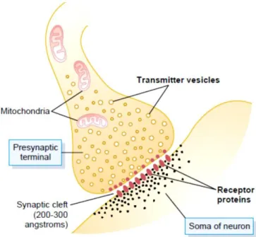
The chemical synapse is the most common in the Central Nervous System of a human (Guyton and Hall, 2000). In the chemical synapse the incoming signal is transmitted when an amount of neurotransmitter is released into the synaptic cleft by the pre-synaptic neuron, it is detected by the second neuron (pos-synaptic neuron) through the activation of receptors (Cardoso, 2001) (figure1.1.1.1). The signal only travels in one direction.

Figure 1.1.1.1 – Illustration of the interaction of neurotransmitters in the synaptic cleft. (Guyton and Hall, 2000)

The pre-synaptic terminal has two important structures, mitochondria and transmitter vesicles. The vesicles carry the neurotransmitters with the objective to release them into the synaptic cleft, while the mitochondria is the provider of adenosine triphosphate (ATP) – energy supplies to synthesizing new transmitters. There are several neurotransmitters in order to facilitate the internal communication and signal transmission within the brain. The result is different if the pos-synaptic terminal has excitatory receptors or inhibitory receptors.

When an action potential propagates to the pre-synaptic terminal, depolarization of it membrane causes a small number of vesicles to empty into the cleft. The released neurotransmitter changes the permeability characteristics of the pos-synaptic neuronal membrane, and becomes vulnerable to an excitation or inhibition.

So far, more than 40 transmitters substances have been discovered, one of the most important is Dopamine (Guyton and Hall, 2000). A wrong quantity of Dopamine in the cleft, can disrupt the normal balance of neurotransmitters in the synapse, this would interfere with the coordination and smoothness of the movement.

Dopamine is produced in the Substantia Nigra and the effect of this neurotransmitter is usually inhibition. (Seeley et al., 2003) The termination of these neurons is mainly in the Striatal Region of the Basal Ganglia (Guyton and Hall, 2000). In patients diagnosed with Parkinson’s disease, was noticed an asymmetric loss of Dopamine terminals, in the Striatum (WE MOVE - Worldwide Education and Awareness for Movement Disorders, 2011). In a study where the objective was to model the disease developments, the subjects were young drug addicts in MPTP

(1-methyl-4-phenyl-1,2,3,6-tetrahydropyradine). This drug destroyed the dopaminergic neurons in the Substantia Nigra and caused an early Parkinson disorder (Byrne, 1997).

1.1.2.Treatment

Parkinson’s disease does not have a cure; however there is an effective treatment for the symptoms. Unfortunately, no therapy has the capacity to reverse or slow this disease; so far the medication subscribed has the purpose of deliver Dopamine to the brain. Usually, patients are given Levodopa (L-dopa) combined with carbidopa; this last is used to delay the conversion of Levodopa into Dopamine, until it reaches the brain (Seeley et al., 2003).

This Levodopa treatment is the most effective treatment for the motor symptoms. However, this L-dopa treatment doesn’t apply to all patients, and some symptoms do not respond as it suppose to. Problems related with balance and tremors may not improve as expected, but the bradykinesia and the rigidity react better. Anticholinergics may help control tremor and rigidity (NINDS Parkinson’s Disease Information Page, 2011). Also the non-motor symptoms such as depression are very common and important targets of the therapy (WE MOVE - Worldwide Education and Awareness for Movement Disorders, 2011).

There are other drugs such as Bromocriptine, Pramipexole and Ropinirole similar to Dopamine, and the neurons react to it in the same way; however these are still under investigation (Seeley et al., 2003).

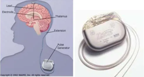
Figure 1.1.2.1 – Deep Brain Stimulation schematic figure and Implantable Pulse Generator. (WebMD, 2002; Parkinson’s Disease Society of the United Kingdom, 2009)

When the chemical treatment does not improve the patient condition, another therapy can be applied, and it is called Deep Brain Stimulation (DBS). In this technique, electrodes are placed in the brain and are connected to a small electrical device that generate a pulse, and it can be programmed externally. These stimulators last between three to five years, depending on the usage. In Parkinson’s disease different places of stimulation have different effects on the symptoms, thalamic stimulation in the ventral intermediate nucleus of the thalamus may reduce limb tremor. When the internal segment of Globus Pallidus (GPi) is stimulated most of the symptoms are reduced (Perlmutter and Mink, 2006), specially the dyskinesias. The subthalamic stimulation usually improves symptoms as tremors, slowness of movements and stiffness. These techniques of surgery vary between treatment centers some are carried with the patient under general anesthesia and some while the patient is awake. One of the three parts of the brain is stimulated with a small electric current and the response is monitored when the tremor is reduced, that confirms the correct target area (Parkinson ’s Disease Society of the United Kingdom, 2009).

A wire is applied with the DBS technique; that is connected to a small unit (figure 1.1.2.1) named as Implantable Pulse Generator (IPG) which is implanted under the skin near the collarbone. It works similar to a pacemaker. The device contains a battery and it generates the electric signal for the stimulation. This stimulation is programmed by a clinician; however on a day to day the patient can control the stimulation with an “ON-OFF” mechanism, using a magnet. When the stimulation is switched “ON”, the electric signals are sent to the brain in order to reduce the PD symptoms (Parkinson’s Disease Society of the United Kingdom, 2009).

DBS can reduce the amount of Levodopa needed, and it is possible to minimize side effects caused by this medicine. One of the side effects of Levodopa is the involuntary movements.

1.2.Anatomy and Physiology of the Motor Cortex

Figure 1.2.1 – Segmentation of the brain, location of the Motor Cortex. Also can be seen the Primary Motor Cortex, Premotor Area and Supplementary Area. (Guyton and Hall, 2000)

The Motor Cortex is a portion of the frontal lobe. It is shown in the figure 1.2.1 is divided into three areas: Primary Motor Cortex, Premotor Area and the Supplementary Motor Area. A stimuli applied in the Premotor Cortex or in the Supplementary Motor Area requires higher levels of current to have a movement, and commonly these are more complex movements than a stimulation of Primary Motor Cortex (Byrne, 1997).

1.2.1.Primary Motor Cortex (M1)

It is located in the first convolution of the frontal lobes anterior to the Central Sulcus. It begins laterally in the Sylvian fissure, spreads superiorly to the uppermost portion of the brain, and then dips deep into the longitudinal fissure.

This area is the one that generates neural impulses that control the execution of movement. It does not control individual muscles directly, but appears to control individual movements or sequences of movements that require the activity of multiple muscle groups (Byrne, 1997). The

signals emitted from M1, travel across the midline of the body and activate the muscles in the opposite side.

The Primary Motor Cortex controls different muscle areas such as face and mouth, arm and hands, trunk, feet and leg, dips into the longitudinal fissure, as indicated in the figure 1.2.1. This type of mapping was made based on tests performed during surgeries, stimulating the areas through electric stimulation (Guyton and Hall, 2000).

1.2.2.Premotor Area

Continuing to observe the image (1.2.1), anterior to the Primary Motor Cortex, extending inferiorly into the Sylvian fissure and superiorly into the longitudinal fissure, where it merges with the Supplementary Motor Area. This area is involved in the sensory guidance of movement, and controls the more proximal muscles and trunk muscles of the body. It performs more complex and task-related movement processing than Primary Motor Cortex (Byrne, 1997).

The nerve signals from the Premotor Area are more complex than the ones generated from the Primary Motor Cortex (Guyton and Hall, 2000).

1.2.3.Supplementary Motor Area

This area lies above the Premotor Area, also in front of the Primary Motor Cortex. It is involved in the planning of complex movements and coordinates two-handed movements (Posit Science Corporation - Brain Connection).

1.3.Electroencephalogram (EEG)

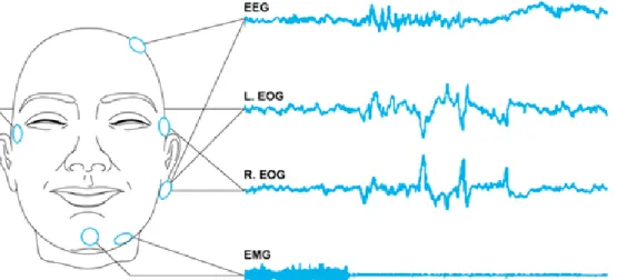
Figure 1.3.1 – Example of electroencephalogram (EEG), electrooculargram (EOG) and electromyogram (EMG) (LaBerge, 2008).

The nervous cells communicate between each other trough electrical signals. These impulses fluctuate rhythmically in distinct patterns. These can be register for an electroencephalograph, which is an instrument that records brain-waves; it was invented in 1929 by a German scientist, Hans Berger. The Electroencephalography records (figure 1.3.1) the voltage changes that result from the ionic currents in the neurons. This technique is commonly used in research and also in diagnoses since it is a non-invasive process for the patient, and also can detect changes in brain electric activity with a good time resolution (figure 1.3.1) (Oostenveld, 2006).

The recordings are made through the use of electrodes on the patient’s scalp, in special cases the electrodes can be subdural or even be in the cortex. The results of the EEG usually are bipolar, potential between two electrodes in different positions in scalp; or unipolar, when the potential is calculated with a neutral electrode or the average of all the channels. The signal is electrically amplified and appears as a graph on paper or in the computer screen.

1.3.1.Electrode Location Systems

In order to uniform the electrodes placement, and standardize reproducibility so that studies could be compared in the future, HH Jasper in 1958 created a system designated as 10-20 system or

system used in EEG studies with Event Related-Potentials (ERP). However, the progression to multi-channels hardware systems and the need of topographic studies with ERP conducted to a need of standardize a larger number of channels, which could support between 21 to 74 electrodes.

Figure 1.3.1.1 – Electrodes distribution through the scalp, with percentages. A lateral view (A) and a above the head view (B) (Malmivuo and Plonsey, 1995).

This system is based on the relationship of the electrode location and the area of cerebral cortex. The numbers in the designation of the system, refer to the distance between electrodes, that are percentages as can be seen in the figure 1.3.1.1. After measuring the perimeter of the patient it is calculated 10% or 20% starting the central point in the skull, Cz. There are two anatomical landmarks for the placement, the Naison which is the point between the forehead and the nose, and the Inion the lowest point of the skull in the back of the head.

The electrodes are represented in the scalp map (figure 1.3.1.2), the letters F, T, C, P, A, and O stand for frontal, temporal, central, parietal, ear lobe and occipital, respectively (Oostenveld, 2006). The “z” is to identify the electrodes in the midline, and the “p” means polar. The numbers are distributed as even numbers (2, 4, 6, 8) in the right hemisphere and the odd (1, 3, 5, 7) on the left.

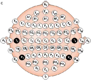
Figure 1.3.1.3 – 10-10 electrode system (Malmivuo and Plonsey, 1995).

To add electrodes it is possible to locate them in the free spaces of the scalp map (figure 1.3.1.3), that is how the others systems appeared, for example the 10-10 system.

The 10-10 system is basically an alteration of the 10-20 system, but this one takes more electrodes using a 10% distance between the electrodes in the scalp, it can take up to 81 electrodes. The nomenclature used in this system was standardized by the American Electroencephalographic Society (Oostenveld, 2006).

1.3.2.EEG signal – Frequency bands

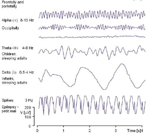
With the EEG signal resulting from the electroencephalograph, it is possible to differentiate frequency bands, such as: Alpha (8-13Hz), Beta (13-30Hz), Delta (0,5-4Hz), Theta (4-8Hz), Gamma (30-100Hz) and Mu (8-13Hz). (see figure 1.3.2.1) The signal can be described as a rhythmic activity or transient activity; in the rhythmic activity the signal is divided into frequency bands, as for the transient activity it is divided as spikes and sharp waves. The frequency bands usually represent some type of physiologic event, as for the spikes can represent an event such as seizure activity.

Figure 1.3.2.1 - Example of the waveforms for the different bands (Malmivuo and Plonsey, 1995).

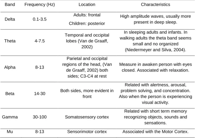
Table 1.3.2.1 – Frequency bands characteristics and respective locations.

Band Frequency (Hz) Location Characteristics

Delta 0.1-3.5

Adults: frontal Children: posterior

High amplitude waves, usually more present in deep sleep.

Theta 4-7.5

Temporal and occipital lobes (Van de Graaff,

2002)

In sleeping adults and infants. In walking adults the theta band seems

small and no organized (Niedermeyer and Silva, 2004).

Alpha 8-13

Parietal and occipital regions of the head, (Van

de Graaff, 2002) both sides; C3-C4 at rest

Measure in awaken person with eyes closed. Associated with relaxation.

Beta 14-30 Both sides, more evident in front

Related with alertness, arousal, problem solving, and concentration. Also when the person is experiencing

visual activity.

Gamma 30-100 Somatosensory cortex

Related with short term memory recognizing objects, sounds and

sensations.

Mu 8-13 Sensorimotor cortex Associated with the Motor Cortex.

The frequency range of the Gamma band is still debated and may lie between 30-60Hz. The signal can differ according with the activity and level of conscience of the subject. As the patient become more active, the EEG signal turns to be higher in frequency and lower in amplitude. If he closes his eyes the alpha activity will dominate the signal. Other situations can been observed in the EEG, for example when a person is dreaming and has active movement of the eyes, also called Rapid Eye Movement (REM). In deep sleep the Delta band turns to be more evident and in cerebral death there is no activity in the EEG (Malmivuo and Plonsey, 1995).

1.3.3.Artifacts present in the Electroencephalogram

The EEG artifacts can induce false conclusions if not removed. The contaminations can occur in different points during the recording. The technological evolution can improve the affectivity of these noise sources in the data, which are usually biological. For example, it will be mention six types of artifacts: eye blink, eye movement, 60 or 50 Hz line noise, muscle activity, pulse and electrocardiogram.

Figure 1.3.3.1 – Eye blink artifact (Knight, 2003).

The artifact known as eye blink is common in EEG (Figure 1.3.3.1), it can be identified by having high amplitude that is usually superior to the signal of interest, also present in all electrodes even the ones in the back of the head. Frequently are recorded in the electrooculargram (EOG), as a pair of electrodes placed around the eye, but these channels cannot be simply subtracted from the contaminated ones since the EOG also have brain signals present (Knight, 2003).

Figure 1.3.3.2 – Eye movement artifact (Knight, 2003).

Also commonly present in EEG is the eye movement (Figure 1.3.3.2), caused by the reorientation of the retinocorneal dipole. The eyeball acts like a dipole with positive and negative poles, cornea and retina respectively. As the globe rotates it generates a large amplitude signal detectable by electrodes (Benbadis, et al., 2012). The eye blink and movement take place in small intervals of time, and with high amplitude (Knight, 2003).

Another noise type is the one introduced by the A/C power supplies (Figure 1.3.3.3). It modifies the data between the scalp electrodes and the recording device. It can be filtered with notch filters but for lower frequency line noise and harmonics this is often undesirable. When the noise or the harmonics are present, in the same frequency of a band of interest, the use of a notch filter for this band can affect negatively the result (Knight, 2003).

Figure 1.3.3.4 – Muscle activity artifact (Knight, 2003).

The muscle activity also known as electromyogram (EMG) (Figure 1.3.3.4) provenience from facial and neck muscles are one type of noise, since the amplitude and the frequency are higher than the signal we desire to acquire. It can affect different sets of electrodes depending on the muscle source (Knight, 2003). Generally, the potentials generated are shorter in time, it can be easily identify by the duration, morphology and frequency (Benbadis, et al., 2012).

Figure 1.3.3.5 – Pulse artifact (Knight, 2003).

Another electric signal that can interfere with the capture of brain signals is the heart beat (Figure 1.3.3.5). It occurs when the electrode is positioned near a blood vessel. The movement of contraction and expansion introduces voltage into the recording, so it can appear as a sharp or smooth wave (Knight, 2003).

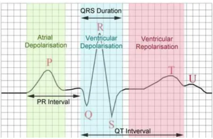
Figure 1.3.3.6 – ECG artifact. (Virtual Medical Centre©_{, 2002 – 2012)}

The last artifact description is the infiltration of Electrocardiogram (ECG), this must be removed in order to obtain a better signal quality. This ECG artifact is related to the heart potentials in the surface of the scalp. The voltage and its appearance vary according to derivation in use, and also montage of electrodes. It is possible to observe this artifact in referential montages using earlobe electrodes A1 and A2. ECG can be recognized by its rhythmicity and or regularity, (each sharp wave represents a QRS complex) (Benbadis, et al., 2012).

1.4.Transcranial Magnetic Stimulation

In the origin of this technique, is the Transcranial Electric Stimulation (TES), which has appeared to activate muscle directly, stimulating the small nerve branches in the muscle through a high voltage electric stimulator (Hallett, 2007). This practice was very promissory in many different purposes, but the subjects felt pain during the stimulation.

A few years later, some difficulties were solved and the stimulation of the brain and peripheral nerves became possible through a magnetic stimulation (Miniussi et al., 2008) now without pain. Transcranial Magnetic Stimulation (TMS) is a noninvasive technique (Lefaucheur and Khedr, 2007), to stimulate the human brain (Hallett, 2007) usually in the Primary Motor Cortex, on conscious subjects and intact scalp (Huang et al., 2005). The Transcranial Magnetic Stimulation can cause temporal and focal changes in the cortical activity (Lefaucheur and Khedr, 2007).

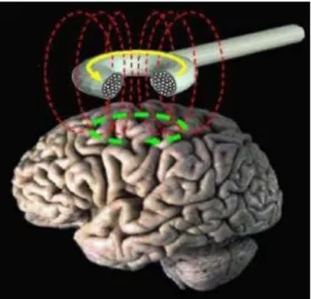
Figura 1.4.1 – Schematic representation of the field and currents involved in Transcranial Magnetic Stimulation. (Braga, 2010)

To better understand how TMS works, observe the figure above (1.4.1), a high electric current (yellow line) produced in the wire coil also designated as magnetic coil, induces a magnetic field (red) perpendicular to the coil, this one placed originally in a way that is tangential to the scalp. This magnetic field can go till 2 Tesla, which is going to cause another perpendicular electric current (green) in the brain tissues. The voltage of the field may excite neurons, which occurs with the induced currents.

There are two types of study with TMS; an online study where the subjects are performing a task while receiving the Transcranial Magnetic Stimulation, and an offline study, when the patient only executes a task after the TMS (Miniussi et al., 2008).

1.4.1.Single, Paired and Repetitive variants of TMS

There are several variants of Transcranial Magnetic Stimulation: single, paired, and repetitive. These produce different effects.

Single pulse-TMS (s-TMS) is able to discharge through a wire coil a high peak and a really quick electric pulse. This means a non-repetitive stimulation. In this technique, the corticospinal neurons are activated trans-synaptically through excitatory interneurons (BioMag Laboratory, 2010; Cantello et al., 2002).

Paired pulse-TMS (p-TMS), this method consists in apply two stimuli through the same coil, separated by interstimulus intervals (Cantello et al., 2002), the intensities of the stimuli can be different (Biomag Laboratory, 2010).

Figure 1.4.1.1 – Schematic representation of the different types of rTMS, 1Hz as Low-frequency TMS, 5Hz as High-Low-frequency TMS, and a patterned example – paired-pulse rTMS. The two

patterns illustrated have 3 pulses of stimulation at 50Hz, repeated every 200ms. The difference between the pattern of iTBS and the basic pattern of TBS (cTBS): the iTBS pattern has a 2 seconds

train of TBS is repeated every 10 seconds, while cTBS has 20 seconds or more train of an uninterrupted TBS. (Huang et al., 2010)

The repetitive TMS (rTMS) as the name suggests is based in a repetitive stimulation to the brain, the stimulation trains are an opportunity to interact more effectively with the cortical tissue (Miniussi et al., 2008). The rate of repetition is very important to the physiologic effect, this is the motive of the parallel classification, according to frequency. If it is below 5 Hz, then it is consider Slow-rate or Low-frequency TMS, above 5 Hz, it is designated as rapid-Slow-rate or High-frequency TMS (Huang

et al., 2010) (figure 1.4.1.1). Several functional neuroimaging studies observed that during and after

this stimulation is detected a suppression or an increase of the cerebral blood flow and metabolism in the stimulated area, for slow and rapid stimulation, respectively (Kobayashi and Pascual-Leone, 2003). The slow r-TMS seems to induce a depressing effect in the motor cortical structures, and for this reason this is appointed to be a possible treatment for epilepsy syndromes. The repetition factor is also one of the main concerns about safety of the subjects, since it is possible to induce seizures (Hallet, 2007) even in normal people (Benninger et al., 2009). There are studies where slow rTMS has been applied to the Motor Cortex with focal, task-specific dystonia, and it restored normal intracortical inhibition and ameliorated function temporarily (Cantello et al., 2002).

In the rTMS recently appeared another technique, named intermittent Theta-Burst Stimulation (iTBS). The basic pattern of Theta burst Stimulation (TBS) consists in a burst of 3 pulses of 50Hz magnetic stimulation at 80% of the active motor threshold given at 200ms. iTBS consists in a

pattern that can be observed in the figure 1.4.1.1, these patterns can produce opposite effects, but more investigations are needed for further conclusions (Huang and Rothwell, 2007). According to the investigation so far conducted, it might be more efficient than the conventional rTMS (Benninger et al., 2009). iTBS can induce larger and longer-lasting changes than rTMS (Huang et al., 2005).

1.4.2.Types of Coil

There are different shapes of coils, this characteristic will influence the pattern of the electric field.

Figure 1.4.2.1 – On the left an 8-figured and on the right a circular coil and respective magnetic field. (Gershon et al., 2003)

The circular coil represented in figure 1.4.2.1 (left) has the strongest current near the circumference, which decreases while approaching the center till reaches zero. Most of these circular coils have a good penetration capacity; however the effect on Motor Cortex is generally asymmetric, (especially with monophasic pulse waveforms). Motor activation is substantially greater on the side in which the coil current flows (from posterior to anterior across the Central Sulcus). The coil is commonly placed at the cranial vertex in order to stimulate both hemispheres at the same time (Hallett, 2007). The stimulation given through this coil is more intensive and covers a larger area of the brain. The most used in clinical and research applications are the circular coils.

The eight-figured coil also known as butterfly consists in two round shapes side by side, as it can be seen in the figure 1.4.2.1 (right). As the current flows in the same direction at the junction point, in this point the induced electric fields are added making this point the maximum. This is the reason that this coil has a more focal stimulation (Cantello et al., 2002; Klein et al., 1999), at defined limit location. The eight-figured coil is a good compromise between efficiency and focability, but the penetration capacity of the induced electric field is limited then the circular coil, since the two side loops are usually smaller (Hallett, 2007).

Another configuration developed is the H form. It is a more specialized type of coil, since it was designed to reduce the field at the cortical surface while augmenting it at depth. However, this objective wasn’t met, since at equal power the penetration was the same as in the eight-figure coil (Hallett, 2007).

The previous coils are used to apply stimulation, when the patient is marked as a placebo in research trials of TMS has led to the development of sham TMS coils. In some research trials, such as a double-blind study, where the sham coil and the real coil cannot be distinguished by the operator, nor the patient. In order to accomplish this requirement the external appearance, the lead wires, the auditory click and mechanical tapping when it fires, as the complex sensations of the scalp muscle contraction and electrical paresthesias that are present in real Transcranial Magnetic Stimulation must be equal or similar.

The simplest form of sham stimulation is to tilt the coil on edge, outside the visual perception of the subject. However, the angle of the tilt and the type of coil may influence 24% to 72% of the resulting field, comparing to the normal positioning of the coil. In this approach it is possible to have the auditory click, but the contact sensation is different, and there is the concern that the reaching field is higher than the 70% of the stimulation, and can produce biological effects.

Actually, there are more possibilities such as visually indistinguishable sham coil, which are placed in the same position as the normal ones. For example the 8-figured coil can be arranged so that the currents are opposite at the coil junction, reducing considerably the induced electric field.

2.State of Art

Parkinson's disease (PD) progression is characterized by motor difficulties which usually respond less to dopaminergic therapy. The Transcranial Magnetic Stimulation has been showing interesting results with Parkinson’s disease. As mentioned before TMS is a recent and very promising technique since it is able to influence brain function if delivered repetitively (Hallett, 2007). The TMS can speed up the reaction time in PD patients (Gaynor et al., 2008). The same can be mentioned regarding the intermittent Theta-Burst Stimulation used in this study, Benninger et al. (2011) while studying the safety of iTBS in PD patients found beneficial effects mainly in the mood, however they did not notice any change in movement or other measures. This therapeutic potential has never been investigated in Parkinson’s disease.

When the stimulus is delivered on the motor cortical areas it can result in a transient inhibition of cortico-motor output (Cunnington et al., 1996). TMS is capable of induce plastic changes in the brain, and is often used to evaluate that capacity (Hallett, 2007). If the repetitive Transcranial Magnetic Stimulation applied is equal or less than 1Hz, the effect predicted is a suppression of the Motor Cortex, while above 20Hz, the cortical excitability seems to be temporarily increased (Kobayashi, Pascual-Leone, 2003). This has an important significance since it can help on the cure or symptoms control of several diseases such as depression, dystonia, stroke and Parkinson’s disease. According to several authors repeated pulses of Transcranial Magnetic Stimulation (rTMS) can change the excitability for minutes or even hours of the corticospinal system. (Hallett, 2007; Thut and Pascual-Leone, 2010)

The study from Khedr et al., (2006) concluded that the 25 Hz rTMS can lead to cumulative and long-lasting effects on motor performance; however there were two groups of patients, one received 25Hz stimulation and another got 10Hz, on early and late stages of PD. They concluded that the 10Hz group improved more than the occipital stimulation group but less than the 25 Hz group. This results were verified during one month, only with a slightly of efficacy.

Another study made by Khedr et al. in 2003, used thirty-six unmedicated PD patients divided in two groups; one submitted to a real stimulation and the other to a sham rTMS. The technique improved several characteristics of movement after the treatments, and the effects lasted one month. Other studies showed successful results, as a study taken by Shimamoto et al. in 1999, where eight patients with a control group, all unmedicated. The stimulus applied consisted in 0,2 Hz, 30 pulses to the right then left cortex, once a week for 9 months, using a circular coil. It was recorded EEG at 3rd, 6th and 9th month. (Cantello et al., 2002)

Another interesting study was taken by Tergau et al. in 1999, with seven subjects medicated without sham stimulation, using a circular coil stimulated at several frequencies. The patients were tested before and after the treatment, but no changes were detected. Similar occurred with Ghabra et

al. in 1999, also failed having positive results, the eleven subjects were off medication 24hours before

the treatment, both sham and real stimulation were used, but didn’t showed significant differences. (Cantello et al., 2002)

It can be concluded that the studies involving the Motor Cortex have a highly variability from one individual to another, resulting in different outcomes.

2.1.Objectives of the Study

The objective of this study is to corroborate if the Transcranial Magnetic Stimulation is a possible alternative treatment for the Parkinson’s disease. As it was mentioned before, it is a very promising non-invasive technique, capable of stimulate the Motor Cortex and other brain areas. For that it was used intermittent Theta-Burst Stimulation, since it was suggested that a more powerful stimulation protocols could enhance efficacy, and would improve gait. A published work (Kuhn et al., 2008) that had a similar purpose, which was inhibit the connection between the Premotor and the Motor Cortex that is abnormal in untreated PD patients. In order to see that, the Power of the Beta band should be lower in the channels C3-P3, F3-C3, Fz-Cz, Cz-Pz, this comparing the first EEG recording with the pos-treatment recordings, this should also reflect in improvements of the motor performance.

3.Materials and Methods

In this study EEG recordings were collected from patients that suffer from Parkinson’s disease and treated with Intermittent Theta-Burst magnetic stimulation (iTBS). This project started with 30 patients, of which only 26 actually participated, with their written consent. The subjects had 40-80 years old; they were picked according with UK-PD-Brain-Bank-criteria, Hoehn-Yahr-stages 2-4 (“off” medication); they were included those who have the slowest gait defined as taking more or equal to 6 seconds walking 10 meters. The exclusion criteria were if any inability or severe freezing detected during that walk distance, and/or also daily falls. Other exclusion parameter was medical or psychiatric illness, history of epilepsy or seizures, pregnancy or metal devices in the head. Screening included EEGs reviewed by epileptologists for pathological activity.

The patients were under an optimal medication with Levodopa-equivalent-dose (LED) more or equal 30 mg, just to remain unchanged during the study.

The stimulation was given to the Primary Motor (M1) and Dorsolateral Prefrontal Cortex (DLPFC) with a circular 90mm-coil, bilaterally. The patients were divided in two groups, one that would receive a real stimulation and another that would get a sham treatment, on both groups the stimulator was out-of-sight. The real stimulation groups of patients received the treatment from Magstim-Rapid stimulator from Whitland, UK; which induced an anterior/posterior – posterior/anterior biphasic current. On the other group there was a sham coil, which produced sound but no magnetic field.

The real and sham iTBS treatments were applied in 8 sessions for 2 successive weeks, one session per day during 4 consecutive days each week. It was constituted in bursts of 3 pulses a 80% of active motor threshold at 50 Hz repeated at 200msec-intervals for 2 seconds, which were repeated 20 times every 10 seconds.

In order to monitor the effects, were recorded EEG data (based in the 10-20 electrode system) from the set of patients, resulting in 85 files, 50 of XLtek and 35 from Nihon Kohden machines. The XLtek machine produced files with a sampling frequency of 500Hz and amplitude measured in mV, while Nihon Kohden files were recorded at 200Hz sample frequency and an amplitude in μV. This measure difference was uniformed by a resampling and rescaling the XLtek files with a Matlab® code. All patients had a baseline recording (BL) recorded before the beginning of the treatment, the second recording (P1) was made after the first stimulation with the objective of check the acute effects of iTBS, and the third file (P2) were acquired after all the treatments, to observe the chronic effects of the therapy. In this study are present the data from 24 patients, since 2 subjects were excluded due to bad quality of the EEG recordings.

Another type of monitoring was performed on the previous day and after each stimulation, according to the study protocol. The tests consists in gait evaluations, similar to inclusion criteria;

bradykinesia where it was assess the time it takes to coordinate hand and arm movements; time of reaction, depression and quality of life appreciation.

The study and data files were provided by National Institute of Health (NIH) in the United States of America (USA). All use of patient material was approved by the Internal Review Board of National Institute of Neurological Disorder and Stroke of National Institutes of Health (decision number 08N0212).

3.1.Preprocessing data

The preprocessing phase is very important since it can affect the results obtained with the Independent Component Analysis (ICA), in the next step. EEGLAB, a computational tool available for Matlab®, was the open source software chosen for this step.

Starting with the rejection of artifacts, were used two different methods, manual removal for the bigger bursts prominent from muscle noise (EMG), and only if present in all the channels at the same time. The EEGLAB allows the user to select a portion of data affected with artifacts and remove it, clipping the two pieces of data.

3.2.Independent Component Analysis

Another way to remove artifacts from data is applying Independent Component Analysis (ICA) to a multichannel EEG recording, removing several contributions of unwanted sources onto the scalp electrodes. Using linear decomposition concepts it assumes that:

- Spatially stable mixtures of the activities of temporally independent cerebral and artifactual sources;

- The potentials detected by the electrodes must be linear;

- No time differences, this means the delays from sources are negligible.

These assumptions are valid for EEG and EMG data. It is also important to have a reasonable amount of data. Since ICA uses spatial filters, does not need a reference channel. (Delorme and Makeig, 2004)

The best example to explain the capacity of Independent Component Analysis is a cocktail party, where there are N different people speaking at the same time in a room, and with N microphones capturing the sound, assuming that the microphones and the people are in the same place during the recording, and that there are no time delays or echoes, ICA can identify the voices (figure 3.2.1).

Figure 3.2.1 – Schematic figure on the mechanism of ICA (Gosselin, et al., 2010).

Independent Component Analysis (ICA) is a method capable for finding underlying factors or components from multivariate statistical data, as it can be observed in figures 3.2.2 to 3.2.4. The mechanism of ICA consists in, a piece of original data, from that is computed a linear component matrix, that is possible to plots scalp maps to help identify the component sources, that can be removed as desired. The result is the most corrected piece of data, without the components artifacted.

Figure 3.2.2 – Representation of the ICA decomposition of the signal in components and respective scalp plots (Jung and Makeig).

Figure 3.2.3 – Representation of the ICA components to be rejected as artifact the result artifact corrected EEG (Jung and Makeig).

Figure 3.2.4 – Illustration of the mechanism of ICA : original EEG, time course ICA components and resulting EEG (Jung and Makeig).

After the preprocessing described above, all the files were computed by this algorithm with the objective to remove other forms of artifacts such as EOG, focal EMG, ECG if present, and line noise at 60Hz. In order to confirm the efficacy of this step another ICA was run and different components could appear and be removed.

3.3.Time Frequency Analysis

In order to make a time frequency analysis it is needed to understand the basis about the main tool used, which was the Fast Fourier Transform (FFT).

The Fast Fourier Transform (FFT) was a tool used during the data processing in this study and is a very complex algorithm, it will only be mention the basis. The FFT is a discrete Fourier transform (DFT) algorithm, which reduces the number of computations needed (Smith, 1997). The

Discrete Fourier Transform (DFT) decomposes a succession of values into components at different frequency, with a considerably big data set, it might take some time. The FFT gets the same results using other approaches, more efficiently and reducing the computation time.

On a first step, the Fast Fourier Transformation decomposes an N points time domain signal into N time domain signals each composed of a single point. After this, it is calculated the N frequency spectra which corresponds to these N time domain signals. Lastly, the N spectra are synthesized into a single frequency spectrum (Smith, 1997).

The FFT algorithm was used to transform the time domain of the EEG recordings to the frequency domain. To apply this to the data, were used a Matlab® code, transforming all the channels acquired and preprocessed with the functions available in EEGLAB as mentioned before.

To begin with the analysis the signal were divided in epochs of 10 seconds with a 50% overlap. To each epochs were applied a Hann window to eliminate the discontinuities in the pieces of signal. The epoched signal was transform into the frequency domain using a FFT, with a frequency resolution of 0.1Hz (2048points), in an interval of 0 – 100Hz. After this the mean of all frequency epochs were calculated to each channel, resulting in one epoch of mean values. The mean signal was divided in frequency bands and the total power computed.

This process was performed by João Careiras, another student involved in the project. He built the Matlab® code capable of the FFT transformation, the frequency bands division and posterior average.

3.4.Statistical Methods

Statistical methods were used in order to better interpret the adquired data. All this analysis was made in SPSS® version 17.0.

Regarding the type of data collected, the first statistical analysis used was a Repeated Measures ANalysis Of VAriance (ANOVA), which is an extension of the dependent t-test, for non independent samples. This test compares three or more group means where the participants are the same in each group in other words, i.e. associated samples. It is the proper test for situations when the subjects are measured multiple times to see changes to an intervention or when participants are subjected to more than one condition/trial and the response to each of these conditions is to be compared (Lund Statistics , 2010).

This type of ANOVA analysis has some requisites such as: all samples must be normality distributed, all samples should have equal variances, and Mauchly test to reflect on the sphericity of

the data. The Repeated Measures ANOVA is especially susceptible to the violation of assumption of sphericity. It relates whether there are any differences between population means.

The null hypothesis (H0) states that the means are equal (equation 1); μ represents the

mean of population and k represents the number of related groups. The alternative hypothesis (Ha)

states that the related population means are not equal (equation 2).

(Equation 1)

(Equation 2)

However, the alternative hypotheses for the study represented below (equation 3); this would be translated as an unilateral test since it is intended to evaluate a decrease not differences.

(Equation 3)

The first step to use the ANOVA Repeated Measures or other parametric test is to assess the normality distribution of all data. To evaluate this was used the Shapiro-Wilk test was used, which is the proper test for samples under 50 elements. When p-value is under 0.05 (for a confidence level of 95%) there is a rejection of the null hypothesis, which means that the distribution is not normal. In this case, the samples must be mathematically transformed and reevaluated. If the transformation does not succeed and in turn the data does not follow the Gaussian distribution, then non-parametric must be employed.

Another condition for this analysis is to study the homogeneity of variance also known as homoscedasticity, with Levene’s test. However this test is not absolutely indispensable to the analysis as Everitt proved in 1996, it was proved that the F test is robust to the violations of homoscedasticity when the number of observations in each group is the same or approximately to 1.5.

Mauchly’s test is one particular requisite of the ANOVA Repeated Measures. It is the formal way to evaluate the assumption of sphericity of the data, and is available in the software chosen for the analysis. If the Mauchly’s test of Sphericity is statistically significant (p<0.05), it means the null hypothesis is rejected and the alternative hypothesis accepted, so the sphericity is violated. In case the sphericity of the data is violated according to the Mauchly test, other methods have been developed which means that can still proceed by using a correctional adjustment called Greenhouse-Geisser (Lund Statistics, 2010). Another correction of the sphericity available is known as Huynh-Feldt test and it is equivalent to the Greenhouse-Geisser mentioned. Both of them adjust the degrees of freedom in the ANOVA test in order to produce a more accurate p-value. In order to use these corrections the estimate of epsilon must be checked, this will help to decide if the sphericity is violated according to the corrections (Pickering, 2011).

As it was mentioned before, when the normality tests fail with the mathematical transformations, it is required to use non-parametric tests. The non-parametric tests are usually used

when the dependent variable is nominal or ordinal but it can also be used with a variable scale. These types of test do not require the normal distribution or the homogeneity of variance.

The Friedman test is homologous to the Repeated Measures ANOVA in the non-parametric tests. It is specialized in more than 3 related samples, it analysis the variance according to rank. To apply this test it must be guaranteed that: the sampling method is random, the independent sample is nominal, and the data distribution for each group has a similar form according to a Box-and-whisker graph.

Another analysis is the comparison between the groups, in order to achieve that a t-student test was performed between the specific groups on each desired pair of data. The t-student test performs a comparison between the means of two independent samples. In this test the null hypothesis is bilateral since it is pretended to know if there are any differences between the groups and not to know if the total power is higher or lower. One of the most important requisites for this test is to be normally distributed.

The null hypothesis is represented in equation 4, while the alternative hypothesis tests the possibility of the means on different groups being different (equation 5).

(Equation 4)

(Equation 5)

In order to evaluate the groups on non-normally distributed samples, it was used the Mann-Whitney U test, which requisites are: random sampling, independence of the samples, and two samples should be similar.

Another used non-parametric test was Wilcoxon, which is the extension of the t-student test for related samples. This was applied when the requirement of normality was not fulfilled; in order to use this test the samples must be related. The null hypothesis is that the difference between both paired samples is zero.

4.Results and Discussion

The objective of this study was to prove if there was a change in the observations post-stimulations comparing two groups, the real stimulation and the sham group. In the first four figures (4.1 to 4.4) the difference between the time stimulations (Baseline, P1 and P2) for the different frequency bands can be seen. The channels chosen are F3-C3, C3-P3, Fz-Cz and Cz-Pz, in other words the ones near to the Motor Cortex and the vertex of the scalp.

Figure 4.1 - Plots of the total power (µV) results from the two types of stimulation, sham (left) and real (right), distributed in baseline (BL), first EEG recording (P1) and the second EEG recording (P2), for the channel F3-C3.

To

tal

P

o

w

er

To

tal

P

o

w

er

BL P1 P2 BL P1 P2 BL P1 P2 BL P1 P2 BL P1 P2 BL P1 P2 Delta Theta Alpha Low High Gamma Beta Beta

Figure 4.2 - Plots of the total power (µV) results from the two types of stimulation, sham (left) and real (right), distributed in baseline (BL), first EEG recording (P1) and the second EEG recording (P2), for the channel C3-P3.

To

tal

P

o

w

er

To

tal

P

o

w

er

BL P1 P2 BL P1 P2 BL P1 P2 BL P1 P2 BL P1 P2 BL P1 P2 Delta Theta Alpha Low High Gamma Beta Beta

Figure 4.3 - Plots of the total power results (µV) from the two types of stimulation, sham (left) and real (right), distributed in baseline (BL), first EEG recording (P1) and the second EEG recording (P2), for the channel Fz-Cz.

To

tal

P

o

w

er

To

tal

P

o

w

er

BL P1 P2 BL P1 P2 BL P1 P2 BL P1 P2 BL P1 P2 BL P1 P2 Delta Theta Alpha Low High Gamma Beta Beta

Figure 4.4 Plots of the total power (µV) results from the two types of stimulation, sham (left) and real (right), distributed in baseline (BL), first EEG recording (P1) and the second EEG recording (P2), for the channel Cz-Pz.

To

tal

P

o

w

er

To

tal

P

o

w

er

BL P1 P2 BL P1 P2 BL P1 P2 BL P1 P2 BL P1 P2 BL P1 P2 Delta Theta Alpha Low High Gamma Beta Beta

From the observation of figures (4.1 to 4.4), apparently there are no differences between the real stimulation and the sham stimulation. On the first figure regarding the channel (F3-C3), the bars P1 and P2 are slightly lower than the Baseline, except for the Gamma band, in real stimulation, as for sham stimulation the P1 is higher than the baseline and P2; also the standard deviation bars are higher which makes these results less significant. As for the channels C3-P3 the plots are leveled, which shows no difference between the control and the treated groups, as no differences are shown between the Baseline and the other recordings. Regarding the Fz-Cz channel the BL, P1 and P2 bars are leveled for the sham stimulation, however the real stimulation P1 is higher than the baseline, and P2 is lower than Baseline and P1. In the last figure, the channel Cz-Pz, the real stimulation, the frequency bars appears to be leveled especially on the beta band.

In the trend plots (figures 4.5 to 4.8) it is interesting to observe the evolution of each patient on the three EEG recordings. Notice that every line is a patient. The Total Power was calculated and distributed for five frequency bands: delta, theta, alpha, low beta and high beta.

Figure 4.5 – Here are represented the trends for the sham (red) and the real (blue) stimulation to the channel F3-C3. Y- axis: total power (µV).

Figure 4.6 - Graphic with EEG total power trends in the channel C3-P3, the red line represents the sham and blue line the real stimulation. Y- axis: total power (µV).

Figure 4.7 - Representation of the trends in the channel Fz-Cz, in the different frequency bands. Real Stimulation in blue and Sham Stimulation in red. Y- axis: total power (µV).

Figure 4.8 – Here are represented the trends for the channel Cz-Pz, in both groups sham (red) and real (blue) stimulation. Y- axis: total power (µV).

On the trend plots (figures 4.5 – 4.8) it can be seen that only the alpha band has a tendency to be steady along the recordings. This can be easily explained, since the subjects had to keep their eyes closed during the process, activating the alpha band. As for the Low and High Beta, it would be desirable to see in the real stimulation (marked in blue) that P1 and P2 would be below the Baseline level; however what can be seen is a leveled blue line, in most of the analyzed channels. However these intentions can be more clearly seen in figures 4.9 to 4.12, with the mean of all the patients, represented forward.

A statistical analysis was computed.

Initially, the Shapiro-Wilk test was performed with 5% of significance to verify the normality of the samples, which was confirmed after the mathematical transformation. This transformation use was a log10(x), which turn the data normally distributed as the ANOVA Repeated Measures require. If that

did not turned the sample normally distributed it, the non-parametric tests described in the section 3.4 to evaluate the significance were used. Also the homogeneity of variance was evaluated and confirmed for all samples.

Figure 4.9 – Mean tendency along time for each frequency, channel F3-C3. Y-axis is the total power mean (µV) on the band, and X-axis is the time analysis (BL, P1, P2).

Figure 4.10 – Mean tendency along time for each frequency, channel C3-P3. Y-axis is the total power mean (µV) on the band, and X-axis is the time analysis (BL, P1, P2).

Figure 4.11 – Mean tendency along time for each frequency, channel Fz-Cz. Y-axis is the total power mean (µV) on the band, and X-axis is the time analysis (BL, P1, P2).

Figure 4.12 – Mean tendency along time for each frequency, channel Cz-Pz. Y-axis is the total power mean (µV) on the band, and X-axis is the time analysis (BL, P1, P2).