Mestrado em Engenharia Informática
Dissertação
Évora, 2018
Esta dissertação não inclui as críticas e as sugestões feitas pelo júri
TÍTULO | Digital Forensics Research Using
Constraint Programming
Nome do Mestrando | João Calhau
Orientação | Pedro Salgueiro
Salvador Abreu
Nuno Goes
ESCOLA DE CIÊNCIAS E TECNOLOGIA
Preface
One year ago I embarked on a new journey, something I thought would be much easier than it turned out to be. This dissertation is the result of this year long battle, although it does not mention the long days spent in front of the computer trying to create something I wasn’t sure could be done, it does mention what resulted from those sacrifices.
Acknowledgments
I would like to start by thanking my parents for their support over these five years of university and to thank my girlfriend, Flávia, for being there for me during the last two years as well.
I thank my supervisors, Prof. Salvador Abreu and Major Nuno Goes, because without them this dissertation would not be possible, and Prof. Pedro Salgueiro for guiding me through all the work done during this year and for being there to provide me with new thoughts and encouraging me to take new steps. I also thank him for reviewing every single paper written during this work and for reviewing the dissertation, both in the initial and final phases. Without him this dissertation would be impossible to read and hard to understand.
I would like to acknowledge Departamento de Informática of Universidade de Évora for providing me, and my colleagues, excellent conditions to work in. And finally I would like to thank all my friends for being there for me and for helping me on many occasions.
Contents
Contents xi
List of Figures xv
List of Tables xvii
Acronyms xix
Abstact xxi
Sumário xxiii
1 Introduction and Motivation 1
1.1 Introduction . . . 1
1.2 Digital Forensics . . . 2
1.3 Constraint Programming . . . 2
1.4 Using Constraints on Digital Forensics . . . 2
2 Digital Forensics 3 2.1 Introduction . . . 3
2.2 History of Digital Forensics . . . 4
2.3 Digital Forensics Problem (DFP) . . . 4
2.4 The Digital Forensic Process . . . 4
2.5 Digital Forensics Notorious Cases . . . 5
2.5.1 The BTK Killer . . . 5
2.5.2 Alicia Kozakiewicz Kidnapping . . . 5
2.6 Known Forensics Tools . . . 6 xi
xii CONTENTS
2.6.1 EnCase . . . 6
2.6.2 Forensic Toolkit . . . 6
2.6.3 Computer Online Forensic Evidence Extractor . . . 6
2.6.4 The Sleuth Kit . . . 6
2.6.5 Foremost and PhotoRec . . . 7
3 Constraint Programming 9 3.1 Introduction . . . 9
3.2 History of Constraint Programming . . . 10
3.3 Constraint Programming Concepts . . . 10
3.3.1 Constraint Satisfaction Problem (CSP) . . . 10
3.3.2 Variable . . . 10
3.3.3 Domain . . . 11
3.3.4 Constraint . . . 11
3.3.5 Modeling a CSP . . . 11
3.4 Approaches to Constraint Programming . . . 11
3.4.1 Backtracking . . . 12
3.4.2 Constraint Propagation . . . 12
3.4.3 Local Search . . . 12
3.5 Known Constraint Programming Solvers . . . 13
3.5.1 Choco . . . 13
3.5.2 Gecode . . . 13
3.5.3 Google OR-Tools . . . 13
3.6 Classic Constraint Problems . . . 13
3.6.1 NQueens . . . 14 3.6.2 Sudoku . . . 14 4 Our Approach 17 4.1 Introduction . . . 17 4.2 Methodology . . . 17 4.3 Modeling . . . 19 4.4 Constraints . . . 19
4.4.1 Type, Path and Date Propagators . . . 20
4.4.2 Word Search Propagator . . . 20
4.5 Data Persistence & Caching . . . 21
CONTENTS xiii 5.1 Introduction . . . 23 5.2 Initial Experimental Results . . . 23 5.3 Current Experimental Results . . . 24
6 Conclusion and Future Work 27
List of Figures
3.1 Possible solution to the 8 queens problem . . . 14
3.2 Sudoku puzzle with respective solution . . . 15
4.1 Example of Sorter output for executable files . . . 18
4.2 Example of Mactime output for a 4GB pen drive . . . 18
4.3 Flow diagram . . . 18
List of Tables
5.1 Initial Experimental Results . . . 24 5.2 Actual Experimental Results . . . 25
Acronyms
CSP Constraint Satisfaction Problem PSR Problema de Satisfação de Restrições DFP Digital Forensics Problem
PFD Problema de Forense Digital FTK Forensics Toolkit
COFEE Computer Online Forensic Evidence Extractor TSK The Sleuth Kit
DSL Domain Specific Language
Abstact
In this dissertation we present a new and innovative approach to Digital Forensics analysis, based on Declara-tive Programming approaches, more specifically Constraint Programming methodologies, to describe and solve Digital Forensics problems. With this approach we allow for an intuitive, descriptive and more efficient method to analyze digital equipment data.
The work described herein enables the description of a Digital Forensics Problem (DFP) as a Constraint Satis-faction Problem (CSP) and, with the help of a CSP solver, reach a solution to such problem, if it exists, which can be a set of elements or evidences that match the initial problem description.
Keywords: Digital Forensics, Constraint Programming, Security, Declarative Programming
Sumário
Pesquisa em Forense Digital Utilizando Programação
por Restrições
Nesta dissertação apresentamos uma nova e inovadora abordagem à análise de Forense Digital, baseada em técnicas de Programação Declarativa, mais especificamente em metodologias de Programação por Restrições, para descrever e resolver problemas de Forense Digital. Com esta abordagem, é nos permitida a utilização de um método mais intuitivo, mais descritivo e mais eficiente para analisar dados de equipamentos digitais. O trabalho aqui descrito permite a descrição de um Problema de Forense Digital (PFD) como um Problema de Satisfação de Restrições (PSR) e, com a ajuda de um ”Solver” de PSRs, chegar a uma solução, se existir, que pode ser um conjunto de elementos ou evidências que correspondem à descrição inicial do problema.
Palavras chave: Forense Digital, Programação por Restrições, Segurança, Programação Declarativa
1
Introduction and Motivation
This Chapter briefly introduces all the different topics presented in this dissertation as well as the different tools and techniques used in them.
1.1 Introduction
This dissertation is about a declarative approach to Digital Forensics Problems (DFPs), that relies on the con-straint programming paradigm to both describe and solve a given Digital Forensics Problem (DFP), which in turn allows to find digital evidences that might be related with criminal activities.
The work described in this dissertation provides a declarative description of a Digital Forensics Problem (DFP) and translates it into a Constraint Satisfaction Problem (CSP) which in turn passes through a Solver that finds a solution to the initial problem, if it exists. This solution is composed by all the found files in the system that comply with the given constraints and the number of files can vary, depending on the problem, from various to none.
The approach described must allow for an easy and efficient method to search for relevant information in the contents of digital equipment.
2 CHAPTER 1. INTRODUCTION AND MOTIVATION The Solver used in this dissertation is among the fastest CSP solvers and it was awarded multiple times [1] [2]. It is based on alternating constraint filtering algorithms and makes use of a search mechanisms.
Part of the work presented in this dissertation has been published in a joint communication with Prof. Pedro Salgueiro, Prof. Salvador Abreu and Major Nuno Goes [3].
1.2 Digital Forensics
Digital forensics is a very important discipline in criminal investigations, where relevant evidences are stored in digital devices. The digital forensics tools have become a vital tool to ensure we can rebuild information after a cyber-attack or even if we just want to analyze any type of digital equipment [4].
It is a very complex task to collect evidence/elements in digital equipment, either related to criminal activity or not. Many tools nowadays are able to collect evidence or data in digital equipment, among them some stand out, including EnCase Forensics, Forensics Toolkit (FTK) and Autopsy.
1.3 Constraint Programming
Constraints can be found in our day to day experiences, almost ubiquitous, representing the conditions that restrict our freedom of decision. Constraint programming is a powerful paradigm mostly used to solve combi-natorial problems. We can consider it as a simple way to model real world problems but it can actually turn into a complex challenge when we want to find solutions for the problem that is being solved [5].
Constraint solvers can use the most varied techniques to solve a certain problem, some examples of these are backtracking, local search and constraint propagation. This last one is considered to be the most basic operation when dealing with constraint solving and is used in almost all constraint solvers as a basic step.
1.4 Using Constraints on Digital Forensics
Constraint Satisfaction Problems (CSPs) and Digital Forensics Problems (DFPs) are two study areas that rarely belong to the same topic of conversation. The work described in this dissertation takes this into consideration and tries to understand if modelling a Digital Forensics Problem (DFP) using Constraint Satisfaction Problems (CSPs) is possible and, in case it is confirmed, if it brings any improvements in terms of processing speed and overall ease of evidence/clue discovery
2
Digital Forensics
In this chapter we will introduce the concepts of Digital Forensics Problem (DFP) and electronic evidence. At the same time we will briefly describe the history of digital forensics and its background, the digital forensics process and some known forensic tools used in actual judicial systems.
2.1 Introduction
The collection of evidence/elements in digital equipment is a complex task, even if they aren’t connected to any criminal activity. If that piece of equipment is connected to any type of computer network, with the consequent increase in digital traffic, more difficult it becomes to detect any anomalies or undesirable communications in the network. Thus, the intrusion detection systems have become a very important tool in computer network security [6].
Digital forensics is a synonym for computer forensics, but in a broader sense, it is the collection of techniques and tools used to find evidence in all digital devices instead of only computers, like in computer forensics [7]. To collect evidence or data in digital equipment, there are many tools capable of analyzing a digital forensics image. Among them, one of the most known tools is the EnCase Forensic [8], which is a proprietary and
4 CHAPTER 2. DIGITAL FORENSICS mercial tool, used in many judicial systems. There are also widely known, open source and free access tools capable of accomplishing the same work. The FTK [9] and the Autopsy [10] are two of them.
2.2 History of Digital Forensics
Prior to the 1980s there wasn’t a real definition of Digital Forensics, digital crimes were few, and the few that actually happened were recognized and dealt with using existing laws. Over the next few years the volume of digital crimes started to increase and laws were approved to deal with issues of copyright, privacy/harassment and child pornography [11].
Between the 1980s and the 1990s, the field of Digital Forensics started to grow with the growth of computer crime. This growth caused law enforcement agencies to begin establishing specialized groups, usually at the national level, to handle the technical aspects of investigations [12]. Many of the members of these group mem-bers were law enforcement professionals as well as computer hobbyists, which became responsible for the field’s early initial research and direction [13].
By the end of the 1990s, a demand for digital evidence grew more and advanced commercial tools such as Encase [8] and FTK [9] were developed. This allowed analysts to examine copies of media without using any live forensics [14]. More detailed information about these tools can be found in Section 2.6.
From the 2000s and onwards, a need to standardize tools and procedures began to show and various bodies and agencies, in response to this need, began publishing guidelines for digital forensics [14]. The issue of training also began receiving attention and commercial companies began to offer certification programs. It’s focus also began to change, to a more internet oriented crime, particularly the risk of cyber warfare and cyberterrorism [13].
2.3 Digital Forensics Problem (DFP)
Electronic Evidence or digital evidence is any probative information stored or transmitted in digital form [15]. Such evidence is acquired when data or digital physical items are collected and stored for examination pur-poses [16].
Each different case of digital forensics represents a different DFP. It all depends on the electronic evidence per-tinent to the case in question and the subsequent way that the evidence is treated and processed. The problem with this process is that digital forensics is still a fairly young subject [7], and new investigation procedures are emerging everyday [17]. Add to this the fact that new digital devices are constantly being created and envi-sioned, always evolving, presenting this type of electronic evidence in court gives origin to several unique prob-lems when compared to those that arise with other types of evidence. These probprob-lems, as well as the processes taken to avoid them, are more detailed in Section 2.4.
2.4 The Digital Forensic Process
To present electronic evidence in court, special procedures must be taken that differ from the normal ones used for other types of evidence. This is due to the very specific nature of electronic evidence, which is fragile. By this, we mean it can be easily altered, damaged or destroyed by improper handling or improper examination. However, a universal set of forensic procedures doesn’t exist, as it always differs in some parts from point of view to point of view. According to Susan Ballou’s point of view, electronic evidence needs to pass through 4 distinct phases: collection, examination, analysis and reporting [16].
2.5. DIGITAL FORENSICS NOTORIOUS CASES 5 The collection phase involves all the search, recognition, collection and documentation of electronic evidence [16], like extraction of digital images from electronic devices. This step is very important since these collected evi-dences are what lie as the foundation of the whole process.
The examination phase involves the verification of the integrity and authenticity of the evidence collected in the previous phase. It also involves surveying all of the evidence to determine future procedures and some pre-processing to salvage deleted data, handle special files, filter irrelevant data and extract embedded metadata. This part of the examination is critical [18]. It is also very important to make sure all items of evidence can be traced form the crime scene to the courtroom, and everywhere in between. This is known as Chain of Custody and if it is ever broken it can invalidate the whole forensic investigation process and not make it presentable in court [19].
As mentioned before, procedures always change a little according to the different points of view, and accord-ing to Eoghan Casey and Curtis W. Rose the analysis phase can be broken down further into 3 phases: form an hypothesis to explain the observations, evaluate the hypothesis and draw conclusions. From the examined data, normally, various hypothesis can be drawn and from these hypothesis various predictions can flow nat-urally [18]. Once a likely explanation has been established, the forensic practitioners can move on to the last phase.
The final phase, the reporting phase, involves a written report that outlines the examination process and the data recovered [16] to be handed to someone on a higher hierarchy than the practitioner for validation [18]. After the due validation of the report, the findings may finally be presented to court. Sometimes an examiner may need to testify about the conduct of the examination and the validity of the methods and procedures [16], the validity of the tools used during examination and analysis phases [18] and the qualifications of the examiner himself [16].
2.5 Digital Forensics Notorious Cases
This section looks to identify some of the most notorious criminal investigation cases in which the main tech-nique used to solve said cases was Digital Forensics.
2.5.1 The BTK Killer
One of the most notorious cases that were ”cracked” with digital forensics, is the case of the American serial killer known as the BTK Killer or the BTK Strangler [20]. Dennis Lynn Rader, known as the BTK Killer had the infamous signature of binding, torturing and killing it’s victims (hence ”BTK”). And he was particularly known for sending taunting letters to the police and newspapers describing in detail his crimes. Rader took a decade-long hiatus in 1991 and resumed his criminal activities in 2004 where he was caught because of metadata embedded in a deleted Microsoft Word document on the last floppy disk he sent to the police [21]. The metadata contained Christ Lutheran Church and the document was marked as last modified by ”Dennis” [22].
2.5.2 Alicia Kozakiewicz Kidnapping
Alicia Kozakiewicz is the founder of the Alicia project, an advocacy group designed to raise awareness about online predators, abduction and child sexual exploitation [23]. At the age of 13 she was the victim of an inter-net luring and child abduction that received widespread media attention [24]. Alicia corresponded online to someone she thought to be a boy of 13 years of age, much like her, that was actually Scott Tyree a 38 year old
6 CHAPTER 2. DIGITAL FORENSICS man who lived in Virginia. He approached her in a Yahoo chat room and over the course of nearly a year, Tyree befriended Alicia and established an emotional connection with her [24]. In 2002, Tyree lured her into meeting him and coerced her into his vehicle and drove her back to his home, where he held her captive in his basement where he shackled, raped and tortured Alicia all of this while broadcasting it online, via streaming video [24]. Luckily a viewer recognized Alicia from news stories and contacted the FBI anonymously and provided them with a Yahoo username [23]. From this username the FBI was able to trace Tyree’s IP address and then his street address, and thus saving Alicia later arresting Tyree at his workplace.
2.6 Known Forensics Tools
In this section we introduce a few well known forensics tools and a brief description of them.
2.6.1 EnCase
EnCase is a piece of technology within a suite of digital investigation tools by Guidance Software. EnCase is traditionally used in forensics to recover evidence from seized hard drives, it allows the investigator to conduct in-depth analysis of user files to collect evidence, such as documents, pictures, internet history and Windows Registry Information. Along with this product, Guidance Software also offers EnCase training and certification. EnCase is a paid and proprietary product that has been used in various court systems, such as in the cases of the BTK Killer and the murder of Danielle van Dam [25].
2.6.2 Forensic Toolkit
Forensics Toolkit (FTK) is a free and proprietary computer forensics software made by AccessData, that scans a hard drive looking for various types of information, such as deleted emails and text strings [26]. The toolkit also comes with a standalone disk imaging software called FTK Imager that can be used to save hard disk images in one file, or several and calculate MD5 hash values to confirm the integrity of said disk. The resulting image file(s) can be saved in various formats, that vary from ISO to DD raw.
2.6.3 Computer Online Forensic Evidence Extractor
Computer Online Forensic Evidence Extractor (COFEE) is a forensics toolkit developed by Microsoft, to help com-puter forensic investigators extract evidence from a Windows comcom-puter. It can be installed on a USB flash drive or other external disk drive and used from there. It acts as an automated forensic tool during a live analysis. COFEE and COFEE online technical support, is free for law enforcement agencies [27].
Unfortunately, in 2009, copies of Microsoft COFEE were leaked onto various torrent websites. Analysis of the leaked tool indicated that it was largely a wrapper around other utilities previously available to investigators [28].
2.6.4 The Sleuth Kit
The Sleuth Kit (TSK) is a free and open-source C library and a collection of tools that allows the analysis of disc images and restore files from them. The TSK framework is what Autopsy [10], the forensics tool mentioned earlier, uses in it’s background jobs. The TSK framework allows the user to incorporate additional modules so
2.6. KNOWN FORENSICS TOOLS 7 he can analyze file contents and build automated systems. In addition, the library can be embedded in larger digital forensics tools and command line tools can be used directly to find any kind of proof [29].
Of all the tools TSK has to offer, the most interesting one is the Sorter, which analyzes a file system and organizes the file by extension. In addition, it provides us details about the organized files, such as the file Inode number. Sorter can also use a separate hash database to ignore files that are known to be good, such as Dynamic-Link Libraries, or dlls, of the windows file system or even know applications.
Another interesting couple of tools in the TSK suite are the FLS and Mactime modules. FLS lists the files and directory names in the image passed as input [30] while Mactime creates an ASCII time line of file activity based on the bodyfile passed as argument via the flag ”-b” [31]. FLS can also display the names of recently deleted files for a directory using the given Inode and it can also extract a bodyfile with all sorts of information about all Inodes found. This last part is interesting because the bodyfile is a slash separated file containing information about every file in the system, which means one can take that file and pass it through mactime. Mactime takes the slash separated file and converts it in a comma separated file with time related information, ordered by Inode number.
Finally, to recover lost files, we can use a rather handy tool called ICAT [32]. This tool opens the image passed as argument and copies the file, specified with the given Inode number, to standard output. This can be particularly useful when used with FLS to extract all the Inode numbers we want to recover.
2.6.5 Foremost and PhotoRec
Foremost is a forensic data recovery program for Linux and it is used to recover lost files by header, footer or data structures. This program achieves this by a process known as file carving, which is the process of reassembling computer files from fragments in the absence of file system metadata [33].
PhotoRec is a free and open-source utility software and much like Foremost, also uses the file carving process. However, it is designed to recover lost files from various digital camera memory [34].
3
Constraint Programming
In this chapter we introduce the concepts of Constraint Programming, Constraint Satisfaction and Constraint Satisfaction Problem (CSP). We also make a brief description of Constraint Programming history, known ap-proaches and tools.
3.1 Introduction
This chapter introduces Constraint Programming, an alternative approach to programming which relies on a combination of techniques that deal with reasoning and computing [35]. Its definition actually comes from the field of Artificial Intelligence, and more specifically, arises from the concept of Constraint Satisfaction.
Constraint Satisfaction, in its most basic form, consists in finding a valid result for each set of problems. These sets of problems are modelled as CSPs which, in turn, specify sets of constraining relations between these prob-lems. CSPs are defined in detail in Section 3.3.
CSPs have been tackled by the most various methods, from automata theory to ant algorithms and are a topic of interest in many fields of computer science [5].
10 CHAPTER 3. CONSTRAINT PROGRAMMING
3.2 History of Constraint Programming
Before understanding what Constraint Programming is, we need to understand that Constraint Satisfaction is the process of finding a solution to a set of constraints that impose conditions that the variables must satisfy [35]. A solution is found when a set of variables satisfies all constrains. These constraints and variables are described in detail in Section 3.3.
Constraint Satisfaction originally appeared in the field of artificial intelligence in the early 1970s. During the 1980s and 1990s constraints started being embedded in programming languages, as they were being developed, and the term Constraint Programming started to take form. Examples of these programming languages are Prologand C++ [35].
In the AI community interest in Constraint Satisfaction developed into two streams, the language stream and the algorithm stream. The first stream refers to the side of Constraint Satisfaction that deals with algebraic equa-tions, constraint statements and declarative languages, while the second stream refers to the actual algorithms used to solve said constrains [5].
3.3 Constraint Programming Concepts
In this section we are going to introduce various important definitions related to CSPs as well how to model them and solve them.
3.3.1 Constraint Satisfaction Problem (CSP)
To solve a CSP one must first model it. A CSP is defined as a given set of n variables to which each is assigned a well defined domain and a set of constraining relations and, in general, more than one representation of a prob-lem as a CSP exists. To solve a CSP one must find all possible n-tuples, such that each n-tuple is an instantiation of the n variables satisfying the relations [36].
There are several definitions we have to delve into to better understand how CSPs work. We need to fully un-derstand what a domain, a variable and a constraint are in this scope as well as how a CSP is defined, modeled and solved.
3.3.2 Variable
According to the field of elementary mathematics a variable is a symbol, usually an alphabetic character, and it represents a number, known as the value of the variable, which can be arbitrary, not fully specified or un-known [37].
In more advanced mathematics, a variable is a symbol that denotes a mathematical object, which could be a number, a vector, a matrix or even a function [38]. Similarly, in computer science a variable is a name (commonly an alphabetic character or a word) representing some value represented in computer memory.
3.4. APPROACHES TO CONSTRAINT PROGRAMMING 11
3.3.3 Domain
According to Hans Hahn, from the field of mathematical analysis, an open set is connected if it cannot be ex-pressed as the sum of two open sets. An open connected set is called a domain [39]. In constraint programming, a domain is an open connected set of variables.
A bounded domain is a domain which is a bounded set, while an external domain is the interior of the comple-ment of a bounded domain [40]. Carlo Miranda often used the term region to identify an open connected set, while reserving the term domain to identify an internally connected one.
3.3.4 Constraint
A constraint is a relation on the domains of a set of variables. It can be viewed as a requirement that states which combinations of values from the variable domains are allowed [35].
During the modeling of a CSP there can be two types of constraints. If the problem mandates that the constraints be satisfied, then the constraints are referred to has hard constraints. However if in the problem it is preferred, but not required, that certain constraints be satisfied, then such non-mandatory constraints are referred to as soft constraints. 3.3.5 Modeling a CSP Listing 1 Modelling a CSP CSP = (V, D, C) V ={V1, V2, . . . , Vn} D ={D1, D2, . . . , Dn}, Vi∈ Di C = (C1, C2, . . . , Ct), Cj = (Ri, Sj)
Listing 1 represents a classically modelled CSP, according to Eugene C.Freuder and Alan K.Mackworth, as a triple CSP = (V, D, C)where V is an n-tuple of variables V = (V1, V2, . . . , Vn), D is a corresponding n-tuple of
domains D = (D1, D2, . . . , Dn)such that Vi ∈ Di, C is a t-tuple of constraints C = (C1, C2, . . . , Ct). A
constraint Cjis a pair (Ri, Sj)where Riis a subset of the Cartesian product of the domains of the variables in
Si[5].
3.4
Approaches to Constraint Programming
In Constraint Programming, we usually have a set of variables, which takes values from an initial domain, to which constraints are applied in order to reduce its domain, and thus reach a solution. Once a constraint is placed on the system it cannot violate another constraint previously applied. This way, we can express the requirements of the possible values of the variables [41].
CSP are typically solved with the help of solvers. These solvers are essentially search algorithms, usually based on backtracking techniques[42], constraint propagation [43] or local search [44].
12 CHAPTER 3. CONSTRAINT PROGRAMMING
3.4.1 Backtracking
Backtracking search is a basic control structure in computer science and finds a particular application in artificial intelligence. As the search is in general exponential in the number of variables, it is particularly helpful to have some means of obtaining bounds on the effort required for individual problems or classes of problems [45]. Backtracking searches incrementally and finds possible candidates to solve the problem. At the same time, it removes the candidates that can not be used as a valid solution to the problem [42]. One of the most used examples for this type of search method is the n-queens puzzle, where a set of n queens should be organized, in a n× n chess board, in such a way that none of the queens can attack each other. Any partial solution that contains two queens that can attack each other is abandoned immediately. The modelling can be seen in Section 3.6.1.
3.4.2 Constraint Propagation
Constraint propagation is the basic operation in Constraint Programming. It is well-recognized that its extensive use is necessary when efficiently solving hard CSPs. Almost all constraint solvers use it as a basic step [46]. Constraint propagation uses semantics of constraints to identify and discard incompatible combinations of val-ues. Such combinations, which are instantiations that cannot be part of any solution, are called nogoods. A typical way to propagate constraints is by reducing the domains of variables or the relations of constraints, re-sulting in a simpler search space to work on because all the nogoods are now identified and can be used to avoid exploration of useless parts in the search space.
Constraint propagation cannot, however, be used on it’s own because it is only used to simplify a problem while maintaining its semantics so as to make it easier to solve. Some other algorithm must be then used to find the solutions or even optimal solutions [43].
3.4.3 Local Search
Local search methods date back over thirty years ago. Applied to difficult combinatorial optimization problems, this heuristic approach yields high-quality solutions by iteratively considering small modifications of a good solution in the hope of finding a better one [47].
Local search methods generally involve going from one solution to another repeatedly, achievable only through a local move, where valid moves can vary from problem to problem. The set of all solutions, reachable from the initial solution S through a local move is called the neighborhood of S. The set of all probable solutions in the neighborhood of S is called its probable neighborhood. To find the optimal solution, a strategy called iterative improvementmoves, on each iteration, to the best probable neighbor (the least costly) until it can’t improve on the current solution [48].
Of course, this strategy has a very obvious drawback, and because of this several ways of alleviating the draw-back have been proposed, such as multi-start iterative improvements and genetic local search [49]. Both of these apply iterative improvements. The first one builds a pool of solutions and returns the best one while the second one discards the least-promising solutions and repeats the process until some stopping criteria is satisfied [48].
3.5. KNOWN CONSTRAINT PROGRAMMING SOLVERS 13
3.5 Known Constraint Programming Solvers
To reach a solution to a CSP a Solver is needed. A various number of Constraint Programming Solvers exist, we present some of the most used ones in this section. Special attention should be placed on Choco, because this is the tool we chose to use in our constraint solving problem.
3.5.1 Choco
Choco is an open source and free access library dedicated to Constraint Programming. It is written in Java and supports several types of variables, including Integers, Booleans, Sets and Reals. It also supports several types of constraints such as AllDifferent and Count, configurable search algorithms and conflict explaining. It aims at describing real combinatorial problems in the form of CSPs and solving them with Constraint Programming techniques. Choco is used for teaching, researching and real life-applications [1] [2].
The first version of Choco was developed in the early 2000s. A few years later, Choco 2 was developed and declared a success in the academic and industrial world. Since then, Choco has been completely re-written and in 2012 the third version of Choco was launched. The current version comes with a simpler API and is called Choco [50] [2].
Choco is among the fastest CSP solvers on the market. In 2013 and 2014, Choco was awarded two silver medals and three bronze medals at the MiniZinc Challenge that is the world-wide competition of Constraint Program-ming solvers [1] [2].
3.5.2 Gecode
Gecode is a free access, open source, portable, accessible and efficient programming environment used to de-velop systems and applications based on Constraints. Gecode, much like Choco, supports various types of vari-ables and constraints, among them are Integers, Float and Sets. These varivari-ables are used to model problems that are then solved with the help of constraint propagators and search algorithms [51] [52].
Gecode is one of the fastest CSP solvers, it won all gold medals in all categories in the MiniZinc Challenges from 2008 to 2012 [52].
3.5.3 Google OR-Tools
Although Choco and Gecode are two of the most widely used libraries, there are also other new tools, such as the Google OR-Tools [53]. Google Optimization Tools or OR-Tools is an interface that puts together several linear programming solver and that counts on the use of several types of algorithms such as search algorithms and graph algorithms. What this library has that is so noteworthy is the fact that it doesn’t let itself be bound by one language. Although implemented in C++, it can be used in other languages like Python, C# or Java [53].
3.6 Classic Constraint Problems
14 CHAPTER 3. CONSTRAINT PROGRAMMING
3.6.1 N Queens
The n queens problem is, fundamentally, placing n chess queens on an n×n chessboard so that no two queens attack each other [54]. A feasible solution for this problem would be one in which no two queens share the same row, column or diagonal [55].
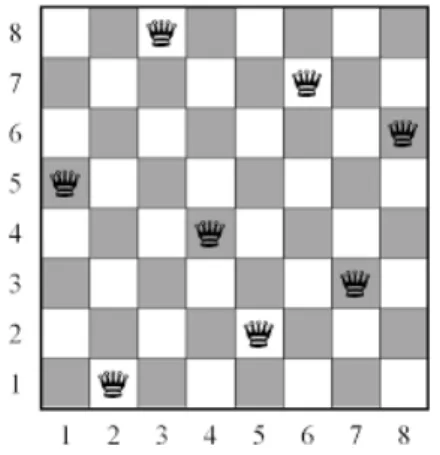
The original n queens problem was introduced by Gauss, in 1850, with an n value of 8 [55] and a total of 72 solutions, but soon after 92 solutions where theorized and in 1874 proved [54]. For a board like this, one of the possible solutions can be seen in figure 3.1.
Figure 3.1: Possible solution to the 8 queens problem
By treating the chessboard as an n×n matrix of square elements, any square can be identified by an ordered pair (i, j)where i and j are row and column numbers respectively. A major diagonal of the matrix can be identified by m− j + i = CONST ANT where the CONST ANT is the number of the diagonal. We can further define a minor diagonal with i + j− 1 = CONST ANT where CONST ANT is the number of the diagonal [55]. The following constraints must always be applied to the n queens problem:
• a) The row numbers are unique. • b) The column numbers are unique. • c) The major diagonal numbers are unique. • d) The minor diagonal numbers are unique.
3.6.2 Sudoku
According to J. Scott Provan, Sudoku is a logic-based, combinatorial number placement puzzle that can be defined by a set S of n grid squares that each have a possible placement of numbers from a set P ={1, . . . , m}, a collection of blocks β where each block consists of a set of exactly m squares and an initial assignment of numbers in some grid squares. The goal is to assign numbers from P to each of the remaining squares of S in a way that each block β has a complete set P of non repeated numbers [56].
The typical Sudoku puzzle has a m× m configuration, and the usual value of m is 9, which brings the value of nto a total of 81 grid squares. On top of having to comply with the constraint of non repeating numbers in a block, the typical Sudoku puzzle also can not have repeating numbers in each row and column.
3.6. CLASSIC CONSTRAINT PROBLEMS 15 One requirement is that every Sudoku puzzle must have exactly one solution [56]. An example of a standard Sudoku puzzle can be seen in figure 3.2 along with it’s solution.
4
Our Approach
This section introduces our approach for modeling a Digital Forensics Problem (DFP) as a Constraint Satisfac-tion Problem (CSP) and reaching a valid soluSatisfac-tion. We describe how we modelled the problem as a CSP, the methodologies used to analyze and extract the information from the digital evidences, the structures used to model the problem and how they are used to reach a solution.
4.1 Introduction
After seeing what a DFP and a CSP are we can finally start modelling a DFP as a CSP to try to reach a valid solution. Like mentioned in previous chapters there are a lot of constraint programming tools, but the one we ended up using was Choco Solver [2]. Along with Choco Solver, we also used the TSK [29] framework mentioned previously.
4.2 Methodology
After acquiring the disk image to be analyzed, it is first processed with the help of tools from the TSK framework, first with Sorter, that can take an hash database form the NIST National Software Reference Library, or NSRL for
18 CHAPTER 4. OUR APPROACH short, that contains all the signatures of traceable software applications (this way we can shorten at the start the number of Inodes that are known to be safe). The sorter creates multiple files with different names, each name being a pre-determined type of file, such as archive, executable or data. After the sorter finishes running, we run Mactime, and it creates a single file containing time information about every file present in the file system. Examples of these files can be seen in Figure 4.1 and Figure 4.2.
Figure 4.1: Example of Sorter output for executable files
Figure 4.2: Example of Mactime output for a 4GB pen drive
The files created by Sorter include all relevant information about the files present in the file system that is being analyzed, including: file path in the file system, the file type, the image name (from where the data was extracted) and the Inode number, which is an internal representation of that particular file in the file system. As for the Mactime file, it only contains date information about each file. This information is parsed into a database that allows the data to be persistent. This database is described in detail in Section 4.5. The data also passes through a caching system that tries to determine if the exact type of constraints have been applied to the file system being analyzed to find if it can skip the lengthily process of trying to find a solution. The caching system is described in detail in Section 4.5.
The whole program can be shortened into the small flow diagram seen in figure 4.3.
Figure 4.3: Flow diagram
After pre-processing the disk image and persisting all necessary data, the DFP, which describes the items that being looked for, is modeled as a CSP. This CSP is then solved by a CSP solver, to reach a solution that satisfies the initial DFP, if it exists. A solution to such a CSP will be a set of file identifiers that match the DFP. It is necessary to use specific constraints to reach the solution mentioned before, which are used to restrict the domain of the variables. These constraints are described in Section 4.4.
4.3. MODELING 19
4.3 Modeling
The problem is modeled as a set of variables that represent the files that need to be found, according to the DFP. These files are represented as numerical values, which are the Inode numbers extracted from the Sorter mentioned previously. Each of these variables are associated with a domain and a set of constraints which are applied to the variables. As previously stated these constraints were created specifically in the context of this work.
In this work we use the Choco Solver, which allows the use of four different types of variables to model the problems: Integers (IntVar), Booleans (BoolVar), Sets (SetVar) and Reals (RealVar). To model a DFP as a CSP, we decided to use Set variables (SetVars). Although the problems are always modelled with one variable, that doesn’t mean we will only have one solution, in fact, SetVars can be instantiated to several values at the same time.
In Choco Solver, SetVars are defined by a domain that is made of two other domains, the Lower Bound (LB) and the Upper Bound (UB). The Lower Bound is a set of integers that must belong to every solution, while the Upper Bound is composed of the set of integers that may be part of the final solution [57]. In our case, when creating the variable with which we are going to work with, the Lower Bound will be left empty. As for the Upper Bound, it will be composed of all the Inodes found during the parsing phase.
Listing 2 Modelling of a Digital Forensics CSP CSP = (V, D, C)
V ={V1, V2, . . . , Vn}
D ={D1, D2, . . . , Dn}, ∀Di∈ D : Di ={Y1, Y2, . . . , Yz}
C ={C1(Vi, . . . , Vj), . . . , Ck(Vi, . . . , Vj)},
∀Ck∈ C : Ck={CP1(Vi, . . . , Vj), . . . , CPz(Vi, . . . , Vj)}
Listing 2 presents a formal representation of a digital forensics CSP, represented by the triple CSP = (V, D, C). V is the set of variables, which represents the files to be found, D is the set of domains for each variable which, where each Di ={Y1, Y2, . . . , Yz} is a set of integer values that represent the Inodes present in the file system;
and C is the set of constraints which restricts the domain of each variable, where each Ckis mapped into a
specific constraint propagator.
4.4 Constraints
To reach a solution, Choco solver makes use of constraints which are implemented as propagators. A propagator declares a filtering algorithm that can be applied to the variables that models the problem, in order to reduce their domain [58]. In the context of this work, we implemented the following propagators:
1. File type: restricts the domain according to the given type of file. 2. File path: restricts the domain according to the given path. 3. Word search: restricts the domain according to the given word. 4. Date: restricts the domain according to the given date.
20 CHAPTER 4. OUR APPROACH All these propagators were implemented to work with the variables used to model the problem: SetVar. To create the propagators, we had to implement the following methods: propagate and isEntailed. The method propagate should restrict the domain according to what we need, while the method isEntailed informs the propagator if a problem has a solution or not, or if it is not possible to determine if a solution exists. These methods are described in detail in Listings 3 and 4.
Listing 3 propagate method for each value in UB do
if value not in database then Remove value from UB end if
end for
Listing 4 isEntailed method if UB is empty then
Problem is impossible to solve else
Problem has possible solution end if
4.4.1 Type, Path and Date Propagators
The Type propagator was the first propagator created and it takes the Upper Bound of the SetVar, iterates over it and removes any Inode that does not belong to the type we are looking for. Path and Date propagators work in the same way. The main difference is what they are trying to restrict: the Type propagator receives the type of file we want to restrict and iterates over the Upper Bound to remove every Inode that does not belong to that type of file, while the Path propagator receives a path and, similarly to the Type propagator, iterates over the Upper Bound and removes every Inode that does not belong to that path. An implementation in pseudo-code of these propagators can be seen in Listing 5.
The type and path propagators have a separate definition that can take more than one input at a time. The separate definition of the type propagator can take more than one type of file so we can look for more than type at a time and the separate definition for the path propagator can take more than one path to search on different folders at the same time.
Listing 5 Type, path and date propagator for var ∈ UB do
Q <= {Query the database if var is of given type, path or date} if Q is null then
Remove var from UB end if
end for
4.4.2 Word Search Propagator
This propagator relies on the Unix4j [59] Java library. This library implements most of the Unix shell commands in native Java. We use this library since it provides efficient methods to find contents inside a file in any file
sys-4.5. DATA PERSISTENCE & CACHING 21 tem. The main method we use from this library is the implementation of the Unix Grep command. We decided to use Grep because we needed a fast and efficient method to search for words in files and seeing as the bash already had a very powerful tool to achieve what we wanted we found the Unix4j Library which permitted us to use bash commands without being in a native Unix environment.
This propagator works in a similar way to the ones previously described. It iterates over the Upper Bound and removes any file that does not contain the word we passed as argument. Also, since this is the last constraint ever being run, we add the Inodes that passed through the propagator to the Lower Bound, because at this moment we’re certain these will belong to the final solution. An implementation of this propagator can be seen in pseudo-code in Listing 6.
Listing 6 Word Search Propagator for var ∈ UB do
Inode <= {Query database to retrieve var information} if I not null then
if [Inode -> name] contains ”word” then Add var to LB
else
G <= {grep -c [Inode => path]} if G = 0 then
Remove var from UB else Add var to LB end if end if end if end for
4.5 Data Persistence & Caching
In an initial developing phase, the database system didn’t exist, and data wasn’t persisted at all. The Inodes where stored in data structures like Hashtables and Linked Lists, and later transferred directly into the array used as the domain of the SetVar used as our variable. This was extremely inefficient, every time we wanted to test a part of the code we would have to run the whole thing and parse the whole information from the Sorter output files, this ended up being one of the reasons why we changed the initial structure of the program. As mentioned before, we decided to use a database to persist data in the case of re-running the code over the same device. This database is created at the time of parsing the data. If the data has not been parsed before, a new database is created for the data being parsed, it can have multiple stored databases for different devices. The database contains five things: 1) the file id (the Inode number); 2) the file name; 3) the file path; 4) the file type and 5) the file date (from the Mactime output).
The caching system was created to lessen the time it takes for the system to solve all the constraint problems it was commissioned to solve by searching in a data structure that contains all the results of previous constraint problems, including the ones that have no results. Every time the system is initiated, it checks if what we’re trying to solve has been solved before, and if so, it skips the whole constraint process and just gives us the results we want, if not it runs like normal and saves the results at the end. This applies to all combination of constraints. These results are being saved in a simple key-value data structure, a hashtable.
5
Experimental Evaluation
In this chapter we are going to talk about the results of the experimental evaluation of the initial program phase. At the same time, we will also present the results of the experimental evaluation of the current development phase.
5.1 Introduction
This chapter presents the experimental results that resulted from two distinct program phases, the initial phase and the current phase. Along with the experimental results, we also present the method through which we extracted the disk images used in said experiments along with a few notes depicting what we could conclude from those results.
5.2 Initial Experimental Results
To evaluate the initial system, we used device images from personal items, including a USB pen drive and an SD card that came from a smartphone. To safely extract and analyze the images from these devices, we used
24 CHAPTER 5. EXPERIMENTAL EVALUATION FTK. After acquiring the images, they were processed with the TSK toolkit sorter to extract their information. They were then sorted into their respective structures and analyzed with the tool developed in the context of this work. The USB pen drive and SD card images have a 4GB and 32GB total size, respectively.
Device Name Time
(sec.)
Total Inodes Found Inodes
Constraints
Pen Drive 0.343 113 2 type
Pen Drive 0.345 113 6 path
Pen Drive 0.387 113 1 type, path
SD Card 36.081 3060 1758 type
SD Card 28.364 3060 6 path
SD Card 24.905 3060 6 type, path
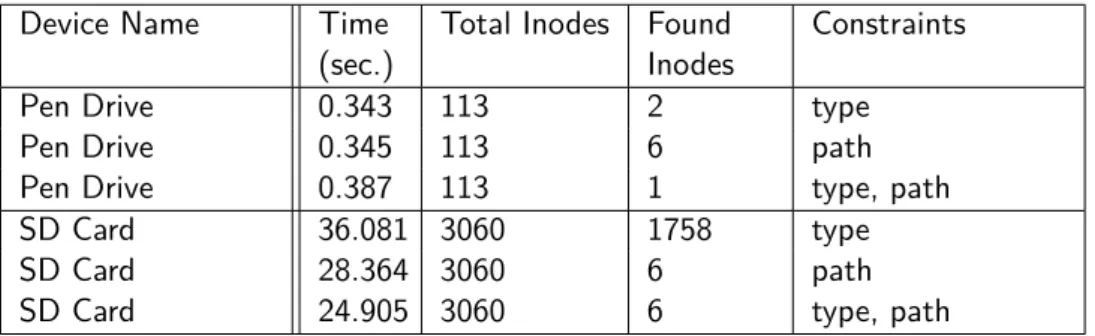
Table 5.1: Initial Experimental Results
The initial evaluation results are presented in table 5.1, which describes the elapsed time to reach a solution in seconds, the total number of files present in the device, number of Inodes Found that match the modeled DFP and the constraints used to model the problem.
We can note that, in this version of the tool, time scaled really poorly with the amount of Inodes to process. This is due to the fact that each time we want to process the Inodes with the tool, they need to be passed pri-marily through each data structure, which are only located in-memory, and then processed with Choco Solver. This process is a lengthy one, even more so with an increase in Inode quantities, a number that in a real world scenario could be in the thousands.
Note that in this early version of the program there were no date and word search propagators, so they are not present in this test. Also no caching system existed, that is why it is not mentioned either.
The constraints used for the pen drive, from top to bottom, are as follow: • 1st test: File type was ”Unknown”.
• 2nd test: File path was ”LVOC/LVOC”.
• 3rd test: File type was ”Unknown” and file path was ”LVOC/LVOC”. The constraints used for the SD card, from top to bottom, are as follow:
• 1st test: File type was ”Audio”.
• 2nd test: File path was ”Music/Disturbed”.
• 3rd test: File type was ”Audio” and file path was ”Music/Disturbed”.
5.3 Current Experimental Results
To evaluate the final version of the tool developed in the context of this work, we used device images from different sources such as, Digital Corpora [60] and Linux LEO [61]. The images taken from Digital Corpora are two, one from a Canon camera, code named ”canon2” and the other a bootable USB disk with a ext3 Ubuntu file system installed, code named ”casper”. From Linux LEO one image was taken, an Able2 Ext2 disk image, code named ”able2”.
5.3. CURRENT EXPERIMENTAL RESULTS 25
Device Name Time
(sec.)
Total Inodes Found Inodes
Constraints Caching
Canon2 0.745 38 33 type no
Canon2 0.677 38 33 type yes
Canon2 1.254 38 36 path no
Canon2 0.836 38 36 path yes
Canon2 0.942 38 33 type, path no
Canon2 0.932 38 33 type, path yes
Canon2 0.911 38 33 type, path, date no
Canon2 0.667 38 33 type, path, date yes
Canon2 0.983 38 33 type, path, date, word no
Canon2 0.930 38 33 type, path, date, word yes
Casper 1.473 1079 79 type no
Casper 0.865 1079 79 type yes
Casper 1.782 1079 5 path no
Casper 0.901 1079 5 path yes
Casper 1.675 1079 4 type, path no
Casper 0.819 1079 4 type, path yes
Casper 1.482 1079 4 type, path, date no
Casper 0.767 1079 4 type, path, date yes
Casper 1.632 1079 4 type, path, date, word no
Casper 0.752 1079 4 type, path, date, word yes
Able2 Partition 3 29.539 11653 14 type no
Able2 Partition 3 0.974 11653 14 type yes
Able2 Partition 3 37.010 11653 66 path no
Able2 Partition 3 0.924 11653 66 path yes
Able2 Partition 3 28.334 11653 12 type, path no
Able2 Partition 3 0.881 11653 12 type, path yes
Able2 Partition 3 26.858 11653 12 type, path, date no
Able2 Partition 3 0.862 11653 12 type, path, date yes
Able2 Partition 3 28.584 11653 2 type, path, date, word no
Able2 Partition 3 0.885 11653 2 type, path, date, word yes
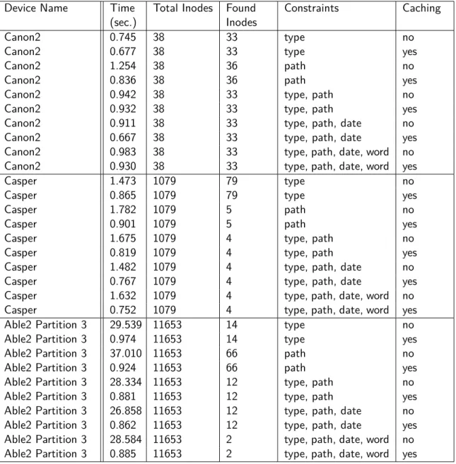
Table 5.2: Actual Experimental Results
The actual evaluation results are presented in table 5.2, which describes the elapsed time to reach a solution in seconds, the total number of files present in the device, number of Inodes found that match the modeled Digital Forensics problem, the constraints used to model the problem and if the caching system was used, for each experiment.
When comparing the two experimental results we can clearly see that the current version of the tool is quite a bit faster than the first implementation, of course this is due to the fact that there is no need to store the Inodes in various structures. This implementation is both faster in terms of processing speed and data persistence, of course these times could be minimized even further if we implemented a database that made use of a faster search method, like for example elastisearch.
The constraints used for the canon2 image, from top to bottom, are as follow:
26 CHAPTER 5. EXPERIMENTAL EVALUATION • 3rd and 4th tests: File path was ”DCIM/100CANON”.
• 5th and 6th tests: File type was ”Image” and file path was ”DCIM/100CANON”.
• 7th and 8th tests: File type was ”Image”, file path was ”DCIM/100CANON” and file date was ”2018-01-01” and onwards.
• 9th and 10th tests: File type was ”Image”, file path was ”DCIM/100CANON”, file date was ”2018-01-01” and onwards and word to look for was .”IMG”.
The constraints used for the casper image, from top to bottom, are as follow: • 1st and 2nd tests: File type was ”Documents”.
• 3rd and 4th tests: File path was ”home/ubuntu/Documents/ssa.gov”.
• 5th and 6th tests: File type was ”Documents” and file path was ”home/ubuntu/Documents/ssa.gov”. • 7th and 8th tests: File type was ”Documents”, file path was ”home/ubuntu/Documents/ssa.gov” and file
date was ”2008-12-30” and onwards.
• 9th and 10th tests: File type was ”Documents”, file path was ”home/ubuntu/Documents/ssa.gov”, file date was ”2008-12-30” and onwards and word to look for was ”pdf”.
The constraints used for the able2 partition 3 image, from top to bottom, are as follow: • 1st and 2nd tests: File type was ”Archive”.
• 3rd and 4th tests: File path was ”lib”.
• 5th and 6th tests: File type was ”Archive” and file path was ”lib”.
• 7th and 8th tests: File type was ”Archive”, file path was ”lib” and file date was ”2000-01-01” and onwards. • 9th and 10th tests: File type was ”Archive”, file path was lib”, file date was ”2000-01-01” and onwards and
6
Conclusion and Future Work
In this dissertation we described a new approach to Digital Forensics, which relies on Declarative Programming approaches, more specifically Constraint Programming, to find evidences or elements in digital equipment that might be related to criminal activities. With this approach, we were able to describe several Digital Forensics problems in a descriptive and intuitive way, and, based on that description, use CSP solvers to find a set of evidences/elements that match the initial problem description in a useful time frame.
The final version of the system presented in this dissertation is quite different from the initial idea, where we had different data structures where the data was saved, no disk persistence what so ever and no caching sys-tem. However, the current version can take a correctly modelled DFP and make use of the Constraint Program-ming paradigm to find its solutions in a way that is intuitive, easy to use and fairly fast to execute. Beyond this there are a couple of other assets that help make the system more reliable: the database, that persists data and the caching system that speeds up the solution finding. Nonetheless, there are some aspects that need to be improved. In a near future, we will use a word indexing system for the word search propagator to improve its performance. We might also consider the creation of special propagators to find hidden messages in image files, as well as the creation a Domain Specific Language (DSL) to make the description of the problems easier for the Digital Forensics analysts. Other than these propositions we could also develop an improvement for the caching system to shorten the processing time even further and a tool to integrate everything.
Bibliography
[1] C. Prud’homme, J.-G. Fages, and X. Lorca, “About choco solver,” 2016.
[2] C. Prud’homme, J.-G. Fages, and X. Lorca, “Choco solver documentation,” 2016.
[3] J. Calhau, P. Salgueiro, S. Abreu, and N. Goes, “Using constraint programming for digital forensics,” 2018. [4] S. L. Garfinkel, “Digital forensics research: The next 10 years,” Digital Investigation, vol. 7, no. SUPPL., 2010. [5] F. Rossi, P. Van Beek, and T. Walsh, Handbook of constraint programming. Elsevier, 2006.
[6] P. Salgueiro, D. Diaz, I. Brito, and S. Abreu, “Using constraints for intrusion detection: The NeMODe system,” Lecture Notes in Computer Science (including subseries Lecture Notes in Artificial Intelligence and Lecture Notes in Bioinformatics), vol. 6539 LNCS, pp. 115–129, 2011.
[7] M. Reith, C. Carr, and G. Gunsch, “An examination of digital forensic models,” International Journal of Digital Evidence, vol. 1, no. 3, pp. 1–12, 2002.
[8] G. Software, “Encase forensic,” 2017. [9] AccessData, “Forensic toolkit,” 2017. [10] B. Carrier, “Autopsy - the sleuth kit,” 2017.
[11] A. Philipp, D. Cowen, and C. Davis, Hacking exposed computer forensics. McGraw-Hill, Inc., 2009. [12] G. M. Mohay, Computer and intrusion forensics. Artech House, 2003.
[13] P. Sommer, “The future for the policing of cybercrime,” Computer Fraud & Security, vol. 2004, no. 1, pp. 8–12, 2004.
[14] E. Casey, A. Blitz, and C. Steuart, “Digital evidence and computer crime,” 2014.
[15] E. Casey, Digital evidence and computer crime: Forensic science, computers, and the internet. Academic press, 2011.
[16] S. Ballou, Electronic crime scene investigation: A guide for first responders. Diane Publishing, 2010. [17] W. H. Allen, “Computer forensics,” IEEE security & privacy, vol. 3, no. 4, pp. 59–62, 2005.
30 BIBLIOGRAPHY [18] E. Casey, Handbook of digital forensics and investigation. Academic Press, 2009.
[19] K. Ryder, “Computer forensics - we’ve had an incident, who do we get to investigate,” SANS Institute InfoSec Reading Room, 2002.
[20] L. Siegel, “Criminology: Theories, patterns, and typologies,” 1998. [21] J. E. Girard, Criminalistics. Jones & Bartlett Learning, 2017.
[22] M. Bardsley, R. Bel, and D. Lohr, “Btk kansas serial killer-full btk story,” World Wide Web. Last accessed, vol. 26, no. 08, p. 2008, 2005.
[23] A. Kozakiewicz, “I, too, am an abduction survivor,” 2013.
[24] N. W. Egan, “Abducted, enslaved—and now talking about it,” 2007.
[25] E. A. Taub, “Deleting may be easy, but your hard drive still tells all,” The New York Times News Service. Re-trieved March, vol. 17, p. 2008, 2006.
[26] P. D. Dixon, “An overview of computer forensics,” IEEE Potentials, vol. 24, no. 5, pp. 7–10, 2005. [27] B. J. Romano, “Microsoft device helps police pluck evidence from cyberscene of crime,” 2008. [28] N. Deleon, “Microsoft cofee law enforcement tool leaks all over the internet!,” 2009.
[29] B. Carrier, “The sleuth kit,” 2017. [30] B. Carrier, “Fls manual page,” 2018. [31] B. Carrier, “Mactime manual page,” 2018. [32] B. Carrier, “Icat manual page,” 2018.
[33] Ruchi, “Recover deleted files with foremost, scalpel in ubuntu,” 2008. [34] CgSecurity, “File formats recovered by photorec,” 2015.
[35] K. R. Apt, Principles of Constraint Programming. Cambridge, 2003.
[36] E. C. Freuder, “Synthesizing constraint expressions,” Communications of the ACM, vol. 21, no. 11, pp. 958– 966, 1978.
[37] K. Menger, “On variables in mathematics and in natural science,” British Journal for the Philosophy of Sci-ence, 1954.
[38] W. V. Quine, “Variables explained away,” Proceedings of the american philosophical society, vol. 104, no. 3, pp. 343–347, 1960.
[39] H. Hahn, Theorie der reellen Funktionen, vol. 1. Julius Springer, 1921.
[40] C. Miranda, Partial differential equations of elliptic type, vol. 2. Springer Science & Business Media, 2012. [41] J. Pearson and P. Jeavons, “A Survey of Tractable Constraint Satisfaction Problems,” Technical Report
CSD-TR-97-15, Royal Holloway, University of London, pp. 1–42, 1997.
[42] D. E. Knuth, “The Art of Computer Programming, Vol. 1: Fundamental Algorithms,” 1997. [43] C. Lecoutre, Constraint Networks: Techniques and Algorithms. John Wiley & Sons, 2010.
BIBLIOGRAPHY 31 [44] R. Dechter, Constraint Processing. Morgan Kaufmann, 2003.
[45] E. C. Freuder, “A sufficient condition for backtrack-bounded search,” Journal of the ACM (JACM), vol. 32, no. 4, pp. 755–761, 1985.
[46] C. Bessière and J.-C. Régin, “Refining the basic constraint propagation algorithm.,” in IJCAI, vol. 1, pp. 309– 315, 2001.
[47] S. Lin, “Computer solutions of the traveling salesman problem,” Bell System Technical Journal, vol. 44, no. 10, pp. 2245–2269, 1965.
[48] N. Jussien and O. Lhomme, “Local search with constraint propagation and conflict-based heuristics,” Arti-ficial Intelligence, vol. 139, no. 1, pp. 21–45, 2002.
[49] J. H. Holland, Adaptation in natural and artificial systems: an introductory analysis with applications to biol-ogy, control, and artificial intelligence. MIT press, 1992.
[50] C. Prud’homme, J.-G. Fages, and X. Lorca, “History,” 2016.
[51] C. Schulte, G. Tack, and M. Z. Lagerkvist, “Modeling and programming with gecode,” Schulte, Christian and Tack, Guido and Lagerkvist, Mikael, vol. 2015, 2010.
[52] Gecode Team, “Gecode: Generic constraint development environment,” 2006. [53] Google, “Google optimization tools web page,” 2017.
[54] I. Rivin, I. Vardi, and P. Zimmermann, “The n-queens problem,” The American Mathematical Monthly, vol. 101, no. 7, pp. 629–639, 1994.
[55] E. Hoffman, J. Loessi, and R. Moore, “Constructions for the solution of the m queens problem,” Mathematics Magazine, vol. 42, no. 2, pp. 66–72, 1969.
[56] J. S. Provan, “Sudoku: strategy versus structure,” The American Mathematical Monthly, vol. 116, no. 8, pp. 702–707, 2009.
[57] Choco-Solver, “Interface setvar api,” 2018. [58] Choco-Solver, “Class propagator api,” 2018. [59] M. Terzer and B. Warner, “Unix4j,” 2018. [60] D. Corpora, “Nps test disk images,” 2018.