A Work Project, presented as part of the requirements for the Award of a Master Degree in Finance from the NOVA School of Business And Economics
ESTIMATION OF CREDIT RISK FOR MORTGAGE PORTFOLIOS: EXPLAINING THE IMPACT OF EXPLANATORY VARIABLES IN MACHINE
LEARNING PREDICTIONS
Field Lab Project Nova SBE & Moody’s Analytics
Carolina Ara´ujo MARTINS, 33251
A project carried out on the Master in Finance Program, under the supervision of:
Moody’s Analytics Advisors
Dr Bahar KARTALCIKLAR, PhD, Risk Modeller - Content Solutions Dr Petr ZEMCIK, Senior Director - Content Solutions
Carlos CASTRO, Senior Director - Economics and Structured Analytics
Faculty Advisor Professor Jo˜ao Pedro PEREIRA
Explanation
The idea of this section is to interpret the trained model. In contrast to Section 4, it is not meant to interpret the model in a technical sense. The goal is to interpret the contribution of each feature to the final prediction. Moreover, this section also sheds some light on feature interactions. It allows banks to align the model results with economic intuition. Moreover, it enables banks to explain the final results to regulating agencies to get eventually the approval to use this model in a production environment.
Theoretical Foundation
Shapley (1953) developed a game-theoretical model to estimate the individual contribution of a player in a game. He proposed for the concept of the so called Shapley value, which is a fair way to distribute the total gain of a game among all player. The main idea is that, most of the time, it is feasible to estimate the marginal contribution of a player. However, the marginal contribution depends on the order that the player entered the game. The last player has most likely the lowest marginal contribution. Shapely values create a permutation of all possible combination and average the marginal contribution among all of them. “The Shapley value is the average marginal contribution of a feature value across all possible coalitions.” (Molnar, 2019). Therefore, the Shapley value can be interpreted as “the average contribution of a feature value to the prediction in different coalitions” (ibid.). However, with the Shapley value, we are not able to draw any conclusion about the models’ performance without this specific feature.
According to Molnar (ibid.), the main advantage of Shapley values is that this approach is the only one which is based on a solid theoretical basis. Moreover, it allows comparing subsets of predictions against each other. This can be especially handy while conducting a fairness analysis. Most importantly, Shapley distributes the deviation from the average prediction fairly among all features. The recently introduced General Data Protection Regulation from the Euro-pean Parliament (Parliament, 2016) requires a right of explanation for any data algorithm. It is not completely clear yet, how this law will be translated into practice. However, it is clear that this will put more pressure on companies, especially in highly sensitive areas like the finance sector, to explain the outcome of models Goodman and Flaxman (2017). Right now, the
Shap-ley values might be the only approach which satisfies all requirements for the GDPR Molnar (2019).
The main points of criticism are the need to access the data to calculate the feature impor-tance. With this approach, it is not possible to make a judgement about a model without the data. Since always all theoretical possible coalitions are used to calculate the Shapley value, it also takes unrealistic data instances into account. Mathematically speaking, this is not an issue for uncorrelated features but could have an impact for correlated feature. To our knowledge, there is no research available about the magnitude of the possible impact. In practical terms, the biggest problem is the computational runtime. Since one has to compute always all of the possible combinations, this can lead, dependent on the size of the dataset, to an unfeasible long time. Approximations for this problem are available, however, they can increase the variance of the Shapley value by a large extend.
Scott M Lundberg and Lee (2017) proposed based on the previous work from Shapley (1953) the SHapleyAdditive exPlanations (SHAP) approach. With this method, it is possi-ble to approximate the Shapley values for every model in a time efficient manner. Scott M. Lundberg, Erion, and Lee (2019)) develop recently a SHAP version specifically tailored for tree based models. With this method, it is possible to calculate exact Shapley values instead of just approximations, while maintaining a reasonable runtime1.
Regardless of the actual implementation, one can sum the absolute Shapley value for a single feature to obtain the global feature importance for the whole model.
Even though SHAP is built inherently around shapely values, it is common in the machine learning literature to refer to the Shapley values as SHAP values. For the sake of consistency, we will follow this approach for the remainder of the paper.
Model Comparison
Machine learning algorithms are proven to be a powerful tool for prediction tasks, however, since the complexity and size of the models imply a loss of interpretability of the results, in many situations, statistics based models are still preferred over the machine learning ones. As
1O(T L2M) to O(T LD2) with M = number of coalitions, T = number of trees, L = number of leaves and D =
mentioned in Section , SHAP appears as a solution for the machine learning black box problem, since it allows for an explanation of the predictions based on feature importance’s both at the individual instance and global levels.
In order to better understand what is the qualitative meaning behind the SHAP values, we start by presenting it’s empirical relationship with the predicted default probabilities.
Figure 1: Relation between the predicted probabilities and the SHAP values.
Figure 1 shows that even though there is not a linear relationship, the predicted probabilities of default and the estimated SHAP values, for both models, follow a sigmoid function. The most important takeaway one should remember for the remainder of the paper is that SHAP values can be translated into probabilities of default. In general, negative SHAP values are directly correlated with a low probability of default while it increases for positive ones. Nevertheless, one has to be careful while comparing different models with each other. Since the graphs appear horizontal shifted from each other, having different SHAP values can still translate to the same impact on the predicted probability of default. However, considering an one unit increase in the SHAP has roughly the same impact in the probability of default for both models, since they assume the same derivative function. Finally, it is possible to observe that, while both models are setting the decision boundary at the 50% level, predictions with SHAP values over 3.5 for the logit model are in default while for the XGBoost the threshold is set at around 1.8.
Figure 2: Feature influences for two individuals. BalanceT oIncome CreditQuality CurrentInterestRate Emplo ymentStatus InterestRateT ype LoanAge MonthsInArrears P aymentFrequenc y Purpose UpdatedL TV Features -0.6 -0.4 -0.2 0.0 0.2 Mean Shapely V alues Performing Loan Model Logistic Regression XGBoost BalanceT oIncome CreditQuality CurrentInterestRate Emplo ymentStatus InterestRateT ype LoanAge MonthsInArrears P aymentFrequenc y Purpose UpdatedL TV Features 0.0 0.5 1.0 1.5 2.0 2.5 3.0 3.5 Mean Shapely V alues Defaulted Loan Model Logistic Regression XGBoost
presented, a default and a non-default. Table 1 shows the characteristics of the two mortgages under analysis.
Table 1: Use-cases’ characteristics.
Feature Non Default Default
Balance To Income 322.85% Missing
Credit Quality Medium Awful
Current Interest Rate 3% 1.75%
Employment Status Pensioner Employed
Interest Rate Type Fixed for Life Floating to SVR
Loan Age 13 102
Months In Arrears 0 2
Payment Frequency Monthly Monthly
Purpose Purchase Purchase
Updated LTV 38.95% 47.94%
Figure 2 shows the SHAP values obtained for each feature for the two individual obser-vations. The bad account refers to a old mortgage with an ’Awful’ credit rating which ends up driving the score up in both models. In comparison, the good-account refers to a relatively younger loan with a lower updated LTV, driving the score in the opposite way. Furthermore, despite the fact that both accounts have the same PaymentFrequency and Purpose, it is possible to observe that, while their influences on the XGBoost are different across the two use-cases, they remain unchanged for the Logit model, reflecting the fact the latter does not account for interactions between features.
Moreover, in order to better understand the differences between the logistic regression and the XGBoost, an average of the absolute SHAP values per feature across all individual predic-tions is taken, resulting in a measure of global feature influence for each model.
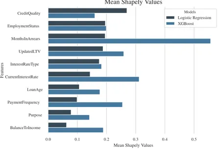
Figure 3: Mean absolute SHAP feature influences. Logistic regression vs. XGBoost.
0.0 0.1 0.2 0.3 0.4 0.5
Mean Shapely Values
CreditQuality EmploymentStatus MonthsInArrears UpdatedLTV InterestRateType CurrentInterestRate LoanAge PaymentFrequency Purpose BalanceToIncome Features
Mean Shapely Values
Models
Logistic Regression XGBoost
From Figure 3 it is possible to observe that the mean feature influences for the XGBoost are systematically higher (with the exception of CreditQuality) than the ones for the logistic re-gression, meaning that the model is assigning more importance to each individual feature. This might be an indicator that it is over-predicting default, which is in line with what is discussed in Sections 4.3 and 4.4. Plus, the general order of features based on their mean SHAP values is also different for both models. However, the comparison at this level might not be totally correct since the models are trained with different datasets (binned and non-binned). A better way to compare the models, is to plot the actual feature influences on the model output, against features values, for each observation.
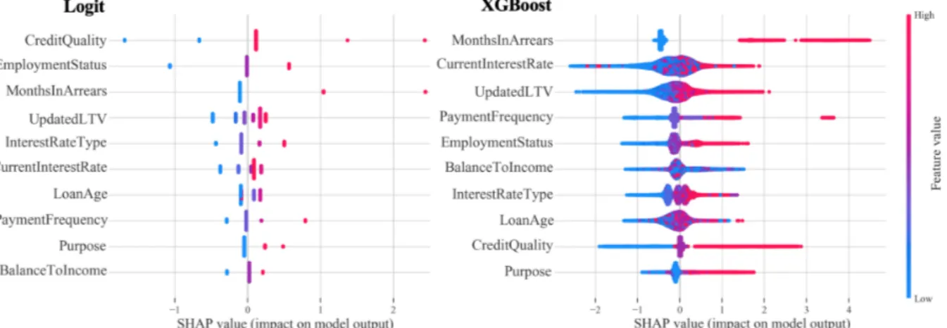
Figure 4 points out one major difference between the two models: the data points are much more sparsed across the SHAP values for the Logit model than for the XGBoost. This behaviour results not only from the fact that the data is binned for the logistic regression but also due to a fundamental characteristic of the boosting algorithm: since this model is able to capture interac-tion terms between features, rather than just correlainterac-tions, the same feature with the same value can assume a different SHAP under different conditions (i.e. if the values of the other features change), giving the impression of a continuous distribution even for categorical features, as can
Figure 4: Feature influences on model outcome. Logistic regression vs. XGBoost. The color-scale represents the variation of the feature, in relative terms.
be seen for InterestRateType.
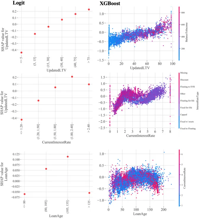
Regarding the relation between feature values and the SHAP2, it is possible to observe from Figure 5 that both models assume similar trends for the variables UpdatedLTV, CurrentInter-estRate and LoanAge. For instance, for the XGBoost, observations with high updated loan-to-value and high BalanceToIncome (represented by more reddish colors) tend to have higher SHAP positive values, while observations with simultaneously low values for both variables (low balance to income represented by the blue dots) correspond to more negative SHAPs. With respect to CurrentInterestRate and LoanAge, variables that assume a non-linear behaviour with the target variable, both models were able to capture the first turn-around point after which the SHAP values start to decrease. Particularly, for current interest rate, one can see that the XGBoost was also able to capture another saddle point while detecting an interesting behaviour in the data: fixed-rate loans are associated high interest rates and tend to have higher SHAP values, which can be explained by the fact that, such loans represent higher risk to the issuer. Moreover, one can infer that the SHAP values have a close relation to the default probability since they assume a similar pattern, across bins, to the coefficients for the statistical regression (Appendix Table A.14), and similar default rate trends (shown in Section 4.4) for both models.
Figure 5: Individual feature influences over feature values. Logistic regression vs. XGBoost. These plots show how the variation of a single feature affects the predictions made by the model. The color-scale corresponds to the variation of a second variable that the model selects to have an interaction effect with the feature under variation (not shown for the Logit model since it is not able to capture such interactions).