2018 | Lavras | Editora UFLA | www.editora.ufla.br | www.scielo.br/cagro
All the contents of this journal, except where otherwise noted, is licensed under a Creative Commons Attribution License attribuition-type BY. http://dx.doi.org/10.1590/1413-70542018423002318
Management zones determination based
on physical properties of the soil
Determinação das zonas de manejo baseadas nas propriedades físicas do solo
Viviana Marcela Varón-Ramírez1*, Jesús Hernán Camacho-Tamayo2, Janeth González-Nivia3
1Universidad Nacional de Colombia, Bogota, Colombia
2Universidad Nacional de Colombia, Ingeniería Civil y Agrícola, Bogotá, Colombia 3Instituto Geográfico Agustín Codázzi, Subdirección de Agrología, Bogotá, Colombia *Corresponding author: [email protected], [email protected]
Received in January 25, 2018 and approved in April 27, 2018
ABSTRACT
The physical characteristics of the soil are defined through the interaction between its properties, and they, in turn, can indicate its physical quality. The study area is located in the Centro Agropecuário Marengo (Marengo Agricultural Center), with an extension of 94.5 ha, subdivided into 17 plots. The objective of this research was to study characteristics such as water storage capacity, structure, consistency, and soil compaction in the two surface horizons (H1 and H2), in order to define management zones through the soil index. Properties such as soil penetration resistance were an indicator of soil degradation, with values higher than 2 MPa in 13 plots. The total porosity exhibited medium or low values in the H1 and H2 horizons, with a predominance of micropores, which means that the presence of water could be lower than 14%. Four management zones were identified for each horizon, where the first zone represents the area where the soil is capable of retaining between 17% and 21% of the available water, with a bulk density of around 1 g cm-3 and organic carbon content close to 6%. By contrast, the fourth zone represents the sites where the soils are the finest, with contents above 45% clay, available water less than 11%, and a mean compaction of 4.39 MPa.
Index terms: Soil degradation; soil compaction; soil water storage; soil index.
RESUMO
As características físicas do solo são definidas através da interação entre seus atributos, indicando sua qualidade física. A área de estudo está localizada no Centro Agropecuário Marengo, com extensão de 94,5 ha, subdividida em 17 parcelas. O objetivo deste trabalho foi estudar as características capacidade de armazenamento de água, estrutura, consistência e compactação do solo nos dois horizontes superficiais (H1 e H2), para definir as zonas de manejo através do índice de solo. Atributos a resistência do solo à penetração, foi um indicador da degradação com valores superiores a 2 MPa em 13 parcelas. A porosidade total apresentou valores médios ou baixos nos horizontes H1 e H2 com predominância de microporos, o que significa que a capacidade de armazenamento de água apresentou valores inferiores a 14%. Foram identificadas quatro zonas de manejo para cada horizonte, sendo que a primeira zona representa a área onde o solo é capaz de reter entre 17 e 21% de água disponível, com densidade do solo em torno de 1,0 g cm-3 e teor de carbono orgânico próximo de 6%. Em contraste, a quarta zona representa os locais onde os solos são os mais finos, com teor de argila acima de 45%, água disponível inferior a 11% e média de compactação de 4,39 MPa.
Termos para indexação: Degradação do solo; compactação do solo; armazenamento de água no solo; índice do solo.
INTRODUCTION
Problems such as erosion, salinization, compaction, and organic carbon loss are processes of soil degradation (Malagón, 2016; Morais et al., 2017) that could be mitigated by monitoring and implementing practices and technologies based on a knowledge of the physical, chemical, biological, and mineralogical properties of each soil.
The soil diversity and the spatial variability of the physical, chemical, biological, and mineralogical distribution properties are the result of the interaction of the formation factors and of several pedogenetic processes (He et al., 2010; Jaramillo, 2011; Cucunuba-Melo;
Álvarez-Herrera; Camacho-Tamayo, 2011). The study of spatial variability and how it relates to production processes is the basis of precision agriculture, which aims to establish a more efficient and sustainable production system (Freitas et al., 2012).
Therefore, the study of the physical properties that define the characteristics such as soil water flow can be an indicator of nutrient movement and crop development (Hincapié; Tobón, 2012). The soil structure and its stability are also degradation indicators, as they are sensitive to management practices (Gabioud; Wilson; Sasal, 2011). Additionally, the interaction and the role of organic carbon (OC) in the conservation of the physical quality of the soil and in the mitigation of degradation processes are important for decision-making regarding irrigation and tillage for a specific area.
Management zones (MZ) are sub-regions in a field where the soil properties are similar and represent similar yield-limiting factors (Moshia et al., 2014; Xiaohu et al., 2016). Agricultural practices based on MZs provide a greater understanding of what the soil offers, and this effort is intended to improve the soil quality and increase production (Betzek et al., 2018). There are several methods for delimiting MZs; multivariate methods are typically used: cluster analysis by C-means and fuzzy C-means (Franzen et al., 2003) and principal component analysis (Moral; Terrón; Silva, 2010; Cohen; Cohen; Alchanatis, 2013).
The results of the analysis and interpretation of soil properties with multivariate methods allow making comprehensive decisions about the management (Anggelopooulou et al., 2013). The use of multivariate analysis techniques allows identifying the possible interaction between variables that apparently are not correlated with each other, since they are a linear combination of the original study variables (Vasu et al., 2016), reducing the analysis dimensionality and defining the variables that determine the variation in the soil, so that they are taken into account at the time of qualifying (Uyan, 2016).
Multivariate analysis techniques based on interdependence methods have been studied and applied in many soil studies. Gustaferro et al. (2010) listed a number of physical and chemical properties of soil that should be taken into account in order to define areas of homogeneous management, based on precision agriculture through the analysis of the principal components.
The objective of this paper was to study properties such as water storage capacity, structure, consistency, and soil compaction in the two surface horizons (H1 and H2), in order to define management zones through the soil index.
MATERIAL AND METHODS
Study area
The Centro Agropecuario Marengo (CAM) is located in the municipality of Mosquera, Cundinamarca,
Colombia, with geographic coordinates 4º42´ north latitude, 74º12´ west longitude and a mean altitude of 2540 m a.s.l. The center has an extension of 94.55 ha. The study area has a dry cold climate and bimodal rainfall distribution, with peaks in the periods from May to June and from October to November, with a mean annual precipitation of 1124 m. The mean temperature in the study area is 12.7 °C (Ordoñez; Bolívar, 2015).
According to Ordóñez and Bolívar (2015), the study area corresponds to three soil orders, Inceptisols, Mollisols and Andisols, with 59%, 28%, and 13% coverage in the area, respectively. Inceptisols are characterized by a degree of evolution between medium and low, and they exhibit umbric epipedons, ochrics, and some mollics. Mollisols have high contents of sodium and endosaturation and episaturation conditions in some of their horizons. The Andisols are deep and well drained.
Study properties and laboratory tests
Field tests and sampling were carried out for the laboratory analysis of the first two horizons (H1 and H2, respectively) in 77 sites, georeferenced with GPS, covering the net area of the CAM plots (Figure 1).
With the samples, the sand (S), silt (Si), and clay (Cl) contents were determined using the pipette method; bulk density (BD) with the clod method; structural stability with the Yoder method to determine of the mean weight diameter (MWD); available water (AW) from the water retention
curves (WRC) obtained with pressure plates; liquid limit (LL) and plastic limit (PL); organic carbon content (OC) with the Walkley Black method and soil penetration resistance (SPR) at H1 and H2 horizons by penetration resistance curves measured with an Eijkelkamp recording penetrometer. For the measurement, a B penetrometer tip (ASAE S313.3, 2009) was used, with an accuracy of 0.05 MPa.
Data analysis
Initially, the central tendency parameters were estimated as mean, median, minimum, maximum, skewness, and kurtosis, as well as dispersion as the coefficient of the variation in CV, in order to analyze the variability of the properties according to the classification proposed by Warrick and Nielsen (1980). These parameters were obtained with the R studio software.
Subsequently, through the use of geostatistical techniques, the structure and the degree of spatial dependence of the properties under analysis were determined via the construction of experimental semivariograms. These semivariograms were fit to theoretical models such as spherical, exponential and Gaussian, where what was observed in the experimental semivariogram was generalized. Subsequently, the spatial distribution of the studied properties and its value for unsampled points was estimated by the use of the Kriging interpolation technique. The geostatistical analysis and the Kriging interpolation were obtained with GS+ software (Gamma Design), and the contour maps were developed using ArcGis 10.0 software.
A multivariate analysis was also carried out based on the physical properties of the soil to delimit management zones, in order to identify the spatial correlations (Aggelopooulou et al., 2013; Rong-Jiang et al., 2014; Raiesi, 2016).
Management zones were delimited by the soil index (SI) through principal component analysis (PCA). PCA seeks to reduce the number of variables, identifying those that define and explain the variance in a data set (Raiesi, 2016), through non-correlated principal components (Vasu et al., 2016). The selection of the principal components that best describe the variability of a soil are those that have eigenvalues greater than one (1) (Rong-Jiang et al., 2014).
The soil index (SI) has been used by different authors in the delimitation of the management zones and the quality of different crops (Ortega; Santibañez, 2007; Camacho-Tamayo; Rubiano Sanabria; Santana, 2013; Uyan, 2016; Vasu, 2016). This method consists of calculating an index for each sampling point, in which the principal components that explain the variance in the data set and the participation of each sampling point of the variance are determined (Equation 1) (Ortega; Santibañez, 2007):
IS w P
z
i ziwhere IS
Z, wi, and Pzi correspond to the soil index at position z, the weight of the standardized variable, and the score factor of the standardized variable, respectively.
Once the SI for each point had been calculated, they were spatialized and interpolated with the Spline or Topo to Raster tool in the ArcGis software. According to the statistical distribution of the SI from the mean and the standard deviation, they were classified into 4 groups.
RESULTS AND DISCUSSION
Spatial analysis
In Table 1, the results of the descriptive statistics for the study variables of the two horizons can be seen. Clay predominates, with 44.49 % of the texture fraction, corresponding to the geomorphology described in the study area (terraced plains, flood plains, and overflow plain), caused by sedimentation processes (Figure 2).
The textural fractions of the soil for the first horizon were adjusted to the Gaussian semivariogram model with a range greater than 700 m. For the H2 horizon, the Cl adjusted the exponential model with a range greater than 700 m. The evaluation of the Kriging interpolation model was high, with a cross-validation coefficient (CVC) greater than 75% (Table 2).
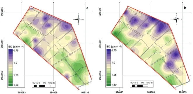
The thickening of a horizon is caused by the illuviation of clays, a genetic process that involves the movement of clays from an upper horizon to an adjacent one (USDA, 2014), a characteristic that can be reflected in the increase of clays in the lower horizon. BD oscillated between 0.77 and 1.39 g cm-3 and between 0.74 and 1.48 g cm-3 for the H1 and H2 horizons respectively, which according to Montenegro and Malagón (1990) are classified from very low to medium.
BD in the two horizons was adjusted to the exponential model with a range of approximately 347 and 348 m and a CVC of 0.62 and 0.85, respectively (Table 2). Adjustment values to the semivariogram and a lower CVC in the H1 horizon are expected, since BD is a property that is sensitive to anthropic intervention, and since the study area is divided into 17 plots with different occupations, spatial variability is expected to be high (Figure 3).
The areas where the greatest BD values, found mostly in the sheep production plots, are due to the cartographic units of soil described by Ordoñez and Bolívar (2015), where they make use of the suffix “d”, which indicates physical root restriction for clay increment (USDA, 2014) in the first horizon nomenclature.
Figure 2: Clay spatial distribution in H1 (a), H2 (b) horizons.
H1 horizon
BD (g cm-3)
Cl
(%) WDM(mm)
LL
(%) (%)PL OC(%) AW(%) (%)TP (MPa)SPR
Mean 1.11 44.49 3.43 62.49 32.95 4.31 0.15 51.90 2.78
Median 1.13 43.12 3.59 60.48 32.03 3.90 0.14 51.22 2.67
Sd 0.14 8.25 1.06 10.51 6.17 2.11 0.06 5.65 1.11
Skewness -0.36 0.10 -0.32 1.41 0.75 0.98 0.93 0.41 0.15
Curtosis -0.34 -0.48 -0.30 2.59 0.63 1.71 0.66 0.09 -0.58
Minimum 0.77 23.22 1.08 46.00 22.00 0.53 0.06 39.62 0.63
Maximun 1.39 62.98 5.75 97.12 53.91 12.30 0.35 67.51 5.17
CV 12.77 18.55 30.96 16.82 18.74 48.96 0.39 0.11 0.39
H2 horizon
BD (g cm-3)
Cl
(%) WDM(mm)
LL
(%) (%)PL OC(%) AW(%) (%)TP (MPa)SPR
Mean 1.10 39.02 2.78 58.11 29.95 3.41 0.14 53.29 3.53
Median 1.12 39.40 2.97 57.32 29.46 3.30 0.13 52.28 3.70
Sd 0.15 10.73 1.28 8.00 5.67 1.31 0.06 6.78 1.31
Skweness -0.49 -0.69 -0.29 -0.15 0.70 0.32 1.47 0.49 -0.01
Kurtosis 0.13 1.29 -1.05 -0.12 3.20 -0.24 2.19 0.24 -0.73
Minimum 0.74 8.08 0.35 38.02 12.65 0.92 0.06 36.48 0.87
Maximum 1.48 60.63 4.89 75.38 52.74 7.00 0.33 69.55 6.41
CV 13.93 27.50 46.29 13.77 18.95 38.49 0.39 0.13 0.37
Table 1: Descriptive statistics for the study properties in each horizon.
Horizon Model Co Co+C Range
(m) R2 Co/(Co+C) CVC
H1
BD (g cm-3) Exponential 0.000 0.018 357 0.730 0.999 0.618
Cl (%) Gaussian 15.400 101.600 758 0.930 0.848 0.948
MWD (mm) Nugget effect 1.090
LL (%) Spherical 16.600 151.600 648 0.782 0.891 0.968
PL (%) Spherical 9.500 46.180 941 0.891 0.794 0.949
AW (%) Spherical 0.613 1.380 622 0.729 0.556 0.601
TP (%) Nugget effect
SPR (MPa) Exponential 0.100 34.500 402 0.772 0.997 0.530
OC (%) Nugget effect 2.460
Horizon Model Co Co+C Range(m) R2 Co/(Co+C) CVC
H2
BD (g cm-3) Exponential 0.000 0.024 348 0.885 1.000 0.846
Cl (%) Spherical 43.400 149.000 701 0.811 0.709 0.912
MWD (mm) Nugget effect 0.960
LL (%) Gaussian 38.600 95.790 950 0.886 0.597 0.889
PL (%) Gaussian 13.700 46.990 1621 0.825 0.708 0.886
AW (%) Spherical 0.001 1.505 148 0.470 0.990 0.729
TP (%) Nugget effect
SPR (MPa) Exponential 0.100 38.650 480 0.739 0.997 0.759
OC (%) Exponential 0.340 1.518 339 0.556 0.776 0.886
Table 2: Semivariogram models parameters for study properties.
BD: bulk density, Cl: clay, WDM: mean weight diameter, LL: liquid limit, PL: plastic limit, OC: organic carbon, AW: available water, TP: total porosity, SPR: soil penetration resistance, Co: nugget, Co+C: sill, CVC: cross validation coefficient.
The lowest BD values for the H1 horizon are found in plots 1, 2, 3, 4, 5, and 6, which have been dedicated mainly to agricultural activities, requiring soil preparation, which in principle favors soil structure, increasing the porous space and decreasing bulk density. Additionally, in these same plots the lowest Cl content in the soil texture can be seen.
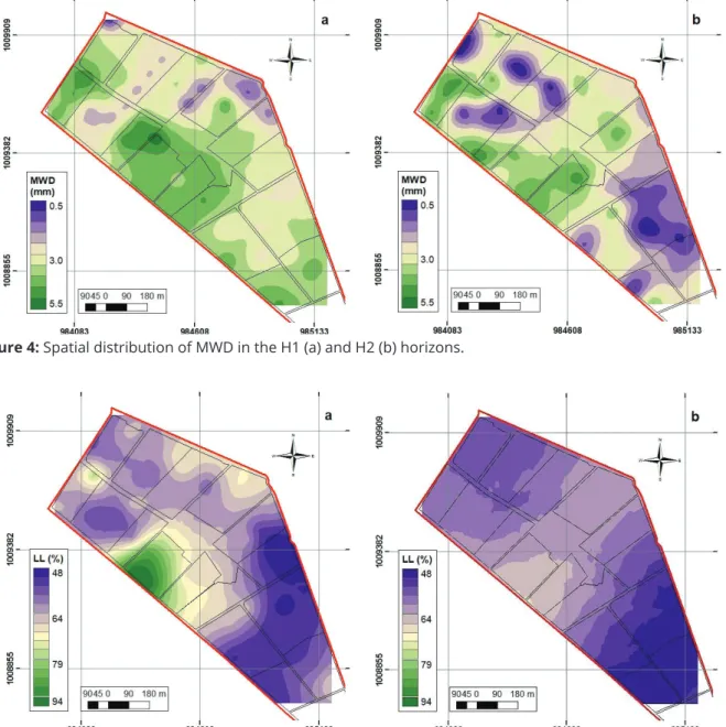
Regarding MWD, it can be seen that most of the study area has aggregates greater than 3 mm in diameter (Figure 4), which indicates stable to very stable structural stability (Malagón, 2016). In contrast, for the H2 horizon
the MWD indicates that the aggregates are considered to be slightly stable to very stable.
These conditions were due to the higher content of OC in the H1 horizon and a higher sand content in the H2 horizon.
In terms of soil consistency, it was found that the mean LL for the H1 horizon has 62.49% water content, with a range between 46% and 97%, and for the H2 horizon a mean value of 58.11%, with a range of water contents lower than 38% to 75% (Table 1). In the liquid boundary spatial distribution (Figure 5), the highest values were observed in
Figure 4: Spatial distribution of MWD in the H1 (a) and H2 (b) horizons.
plots 12 to 14. This is mainly due to the high content of Cl (Stanchi et al., 2015). In addition, these sites show medium to high values of OC, which is linked to the plastic limit when the soil has more than 45% clay. (Moradi, 2013).
The soil AW for the H1 and H2 horizons (15% and 14%, respectively), is at the lower limit of the ranges reported by Allen et al. (2006). For soils with high clay contents, AW values close to 20% are expected, since soil colloids (clays) improve the porosity structure and proportionality, facilitating the presence of mesopores, where water is stored.
Additionally, AW has a 39% CV, which indicates that the useful soil water has moderate variability, and in some places, this property takes its maximum values. This is due to those places where stability and TP are high; otherwise, in places where this property exhibited its lowest range, problems of compaction or thickening were observed.
In Figure 6, it was observed that plots 1, 2, and 3 had medium to high AW values for the H1 horizon and the H2 horizon. According to Ordóñez and Bolívar (2015), these soils correspond to Andisols, which are characterized by their high water storage capacity (Gómez-Rodríguez et al., 2013). This is mainly due to the fact that volcanic material is able to easily fix humic substances (Malagón, 2016), which facilitates the formation of aggregates and therefore its capacity to store water (Martínez et al., 2008).
The TP of the H1 horizon is moderate to high (Table 1) (Montenegro; Malagón, 1990) for plots 1, 2, 3, 4 and 5, due to the parental material of these soils (volcanic material) and low for the other plots, mainly
those dedicated to goat farming, where there should be a predominance of micropores, which mainly define a horizontal behavior in the WRC, also indicating compaction problems in the soil.
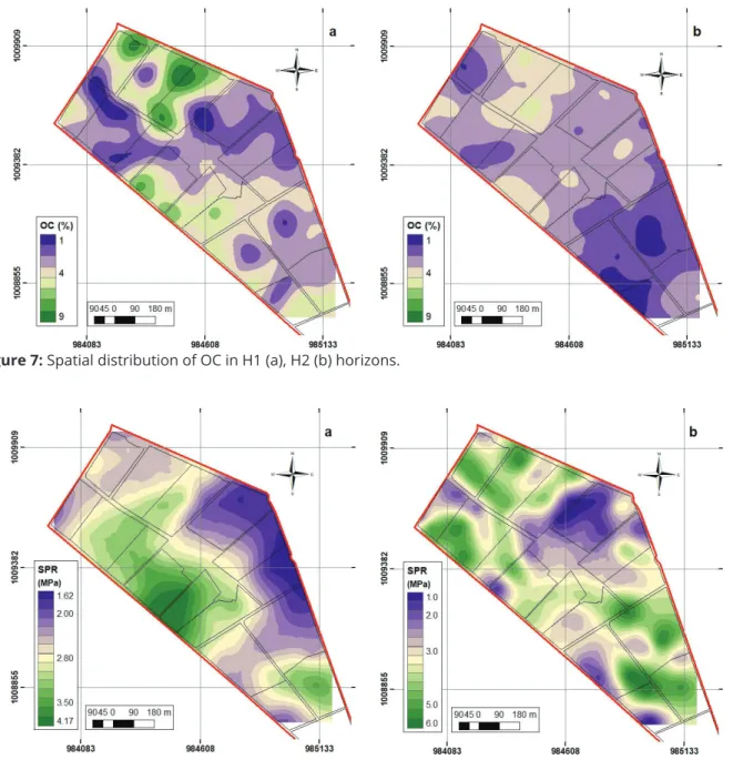
The OC throughout the CAM is at low to very high levels for the H1 horizon and medium to low levels for the H2 horizon. The OC distribution in the H1 and H2 horizons is shown in Figure 7, where two specific areas high in OC are identified. The first of these are in plots 12, 13, and 14, as well as in the southern part of plots 8 and 10, corresponding to the lower areas of CAM, geomorphologically identified as decanting trays (Ordóñez; Bolívar, 2015), where soils have aquic conditions for more than 90 cumulative days per year (USDA, 2014), a condition that impedes the mineralization of soil organic matter (Martínez et al., 2008), while its accumulation in the form of humus is facilitated, depending on the acidity and aeration of water saturation.
The second zone, with high contents of OC (>6%) corresponds to plots 1, 2, and 3, where specifically allophane andisols are found (Ordóñez; Bolívar, 2015). This is because the humic substances produced by the decomposition of the organic matter are stabilized in the soil by means of the absorption of allophane and imogolite in soils of this order (Malagón, 2016).
The places with the highest OC content are associated with the zones where the lowest bulk density values are exhibited, indicating the relationship between the OC content in the formation of aggregates and the distribution of soil porous space (Martínez et al., 2008).
Additionally, in the same areas where the highest OC values were observed, high plasticity indexes were found. This is because OC, like clay, is a colloid of soil and generates cohesion forces, which together with adhesion constitute soil consistency (Malagon, 2016).
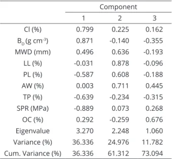
Regarding the SPR in Figure 8, the spatial distribution for the two horizons under study is presented; for the H1 horizon it can be seen that in the plots 12, 13, 14, 15, and 1, high to very high SPRs are exhibited, according to the classification made by Malagon (2016).
This behavior is due to the high Cl content. In addition, soil map units reported by Ordóñez and Bolívar (2015) reveal the presence of vertic intergrades in these zones, a characteristic that indicates a condition of soil consistency from hard to extremely hard during times where the soil is dry.
In contrast, in plots 4, 5, 6, and 7, low SPRs are found (IGAC, 2014), lower than 2 MPa, a condition typical of a soil subjected to tillage processes prior to the establishment and development of crops.
Figure 7: Spatial distribution of OC in H1 (a), H2 (b) horizons.
Component
1 2 3 4
Cl (%) -0.563 0.518 -0.326 0.128
BD (g cm-3) -0.838 -0.010 0.530 0.041 MWD (mm) -0.181 0.589 -0.244 0.381
LL (%) 0.413 0.767 0.334 0.121
PL (%) 0.649 0.494 0.475 0.006
AW (%) 0.680 -0.156 0.192 0.383
TP (%) 0.806 -0.061 -0.559 0.009
SPR (MPa) -0.305 0.518 -0.312 0.088
OC (%) 0.145 0.453 -0.035 -0.820
Eigenvalue 2.870 1.949 1.232 1.005
Variance (%) 31.887 21.651 13.693 11.166
Cum. Variance (%) 31.887 53.539 67.232 78.398
Table 3: Principal component analysis of the physical
attributes for H1 horizon in soil.
BD: bulk density, Cl: clay, WDM: mean weight diameter, LL: liquid limit, PL: plastic limit, OC: organic carbon, AW: available water, TP: total porosity, SPR: soil penetration resistance.
Component
1 2 3
Cl (%) 0.799 0.225 0.162
BD (g cm-3) 0.871 -0.140 -0.355
MWD (mm) 0.496 0.636 -0.193
LL (%) -0.031 0.878 -0.096
PL (%) -0.587 0.608 -0.188
AW (%) 0.003 0.711 0.445
TP (%) -0.639 -0.234 -0.315
SPR (MPa) -0.889 0.073 0.268
OC (%) 0.292 -0.259 0.676
Eigenvalue 3.270 2.248 1.060
Variance (%) 36.336 24.976 11.782
Cum. Variance (%) 36.336 61.312 73.094
1PC 1 0,563% 0,838 D 0,680 0,806 ... 0,145
IS PC Cl B
(2) As for the SPR at the H2 horizon, values higher than
those observed in the H1 horizon were observed in a large part of the study area, which indicates the presence of a hardpan, caused by the combination of pedogenetic processes (translocated clay) and anthropic management (tillage).
Management areas - Soil Index (PCA)
Management areas for the H1 horizon were defined by calculating a soil index based on 4 principal components with eigenvalues greater than one (1), which explained 78.39% of the variance in the properties (Table 3).
The PC1 includes the properties related to the storage capacity of water in the soil, since PC1 is a linear combination with TP, AW, and Cl content and BD. The PC2 mainly expresses the properties related to the soil structure and consistency (MWD, LL, SPR), which explains 21.65% of the total variance (Table 3). The OC is mainly expressed in PC4, which could be a component that describes the storage conditions of OC in the soil.
For the H2 horizon, 3 principal components with eigenvalue greater than one (1) were estimated, which explains 73.09% of the total variance (Table 4). PC1, as in the H1 horizon, describes the properties that determine the storage capacity of water in the soil as a result of its textural composition and porosity.
For each horizon, 4 management zones were defined according to the SI; however, the SI for the first horizon was calculated with the first PC (1PC), first and second PC (2PC), and the four PCs (4PC). Likewise, for the second horizon, the IS was calculated with the first PC (1PC) and the three PC’s (3PC).
Table 4: Principal component analysis of the physical
attributes for the H2 horizon in soil.
BD: bulk density, Cl: clay, WDM: mean weight diameter, LL: liquid limit, PL: plastic limit, OC: organic carbon, AW: available water, TP: total porosity, SPR: soil penetration resistance.
In Figure 9a, the management zones defined by the calculation of a soil index taking into account the CP1 can be seen. This principal component is a combination of the content of clay, BD, AW, and TP (Equation 2), properties that define the storage capacity of water in the soil as a product of the textural composition and the porous space.
Therefore, the management zones 1-1PC and 2-1PC of Figure 9a correspond to the zones where the soil exhibits higher values of BD and Cl content and therefore lower values of TP and AW. In contrast, the areas 3-1PC and 4-1PC represent the places where Cl and BD content is lower, and therefore they have a better distribution of pores and better water storage.
When the management areas are defined by integrating the two principal major components (Equation 3), those areas
1 0,563% 0,838 D 0,680AW 0,806TP ... 0,145OC
are defined which in addition to having the characteristics of the areas defined with the IS1CP have similar structure and
consistency properties (MWD, LL, SPR) (Equation 4).
In Figure 11a, 4 management zones described by PC1 can be seen, which are defined by properties such as texture and porous space distribution of soil, according to Equation 5, which corresponds to the linear combination of PC1 properties.
Figure 9: Management zones defined for H1 horizon with 1PC (a) and 2PC (b).
2PC 1 2
IS PC PC
2 0,589 0,767 0,518 ... 0,453
PC MWD LL SPR OC (3)
(4)
The 1-2PC and 2-2PC zones in Figure 9b, in addition to the properties mentioned above, have small aggregates and moderate to low structural stability. Moreover, the 3-2PC and 4-2PC zones were those with the characteristics of 3-1PC and 4-1PC, which exhibited a higher MWD with moderate to high structural stability and higher LL, which represents an advantage in the mechanization work.
Finally, Figure 10 shows the management zones defined with the 4 principal components (1-4PC, 2-4PC, 3-4PC and 4-4PC). In addition to the aforementioned characteristics, these zones exhibit the other variables of study (OC and PL), properties that have been expressed in the third and fourth principal components. The characteristics of each zone are shown in Table 5. Zone 4 represents the areas where there was a lower BD, lower Cl content, higher TP, and higher AW. However, it is considered that the management zones described with 1PC and 2PC better reflect the behavior of the properties in the field.
The H2 horizon management zones were also defined progressively through the calculation of the soil index, from the first PC and the first three PC. The area was defined in 4 zones as well for the H1 horizon.
1PC 0,799% 0,871 D 0,639 0,889 ... 0,292
IS Cl B
(5)
Zones 3-1PC and 4-1PC correspond to those zones where the BD has lower values as a result of a high TP and low clay content. By contrast, 1-1PC and 2-1PC areas correspond to those places where BD is higher, related to very fine textures and low presence of pores, which agrees with the UCS described by Ordóñez and Bolívar (2015), who report the presence of horizons with “Bd” nomenclature (USDA,
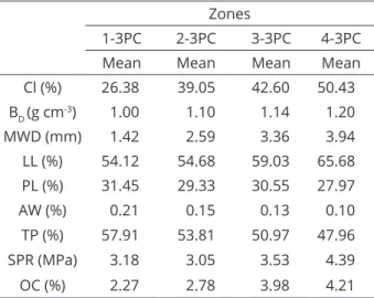
2014), which indicates densified horizons in the same zones. Finally, the soil index of the 3PCs integrates all the study properties in the H2 horizon, in which 4 management zones were also defined, whose properties are described in Table 6 and Figure 11b.
Zone 1-3PC, represents those places where lower values of SPR, lower Cl content, and higher TP and AW were observed. These zones correspond mainly to plot 4, dedicated to the production of fruit trees.
Regarding the structural stability properties of the soil, the aggregates with the largest diameter are found in zones 3-3PC and 4-3PC, and they have a moderate to high structural stability, as a response to a higher OC content for the H2 horizon.
0,799% 0,871 D 0,639TP 0,889SPR ... 0,292OC
It is important to note that the management zones defined by the 2 types of soil indexes (IS1PC, IS3PC) for the H2 horizon are similar and change little in space, reflecting the high correlation observed between the
Figure 10: Management zones defined by 4PC for H1
horizon.
Figure 11: Management zones for H2 horizon with 1PC (a) and 3PC (b).
Zones
1-4PC 2-4PC 3-4PC 4-4PC
Mean Mean Mean Mean
Cl (%) 49.89 45.61 42.93 39.84
BD (g cm-3) 1.30 1.13 1.08 1.01
MWD (mm) 3.44 3.22 3.79 3.43
LL (%) 53.31 58.18 66.32 75.85
PL (%) 26.05 29.65 36.77 42.25
AW (%) 0.09 0.14 0.15 0.23
TP (%) 45.44 51.15 52.66 55.93
SPR (MPa) 2.51 2.87 3.08 2.25
OC (%) 3.60 3.86 4.96 4.24
BD: bulk density, Cl: clay, WDM: mean weight diameter, LL: liquid limit, PL: plastic limit, OC: organic carbon, AW: available water, TP: total porosity, SPR: soil penetration resistance.
Table 5. Properties of management zones defined by
SI in the H1 horizon.
CONCLUSIONS
Principal component analysis helps to establish the MZs by grouping areas that have similar characteristics. The establishment of the MZs through of the soil index was spatially related to the behavior of the soil properties. The MZs exhibited a significant correlation with properties influenced by anthropic management such as BD and TP, as well as with former factors of the soil like the clay content. Finally, for the zones defined with the highest values of BD
and the presence of compacted layers, it is recommended to recover the soil structure through the contribution of organic matter via the incorporation of biomass and its preservation, decreasing its rate of mineralization through practices such as reduced or zero tillage and vegetation cover.
REFERENCES
ALLEN, R. et al. Evapotranspiración del cultivo. Guías para la determinación de los requerimientos de agua en el cultivo. Organización de las Naciones Unidad para la Agricultura y la Alimentación, 2006. 298p.
ANGGELOPOOULOU, K. de et al. Delineation of management zones in an apple orchard in Greece using a multivariate approach. Computers and Electronics in Agriculture, 90:119-130, 2013.
BETZEK, N. M. et al. Rectification methods for optimization of management zones. Computers and Electronics in Agriculture, 146:1-11, 2018.
CAMACHO-TAMAYO, J. H.; RUBIANO SANABRIA, Y.; SANTANA, L. M. Management units based on the physical properties of an Oxisol. Journal of Soil Science and Plant Nutrition, 13(4):767-785, 2013.
COHEN, S. et al. Combining spectral and spatial information from aerial hyperspectral images for delineating homogenous management zones. Biosystems Engineering, 114:435-443, 2003.
CUCUNUBÁ-MELO, J. R.; ÁLVAREZ-HERRERA, J. G.; CAMACHO-TAMAYO, J. H. Identification of agronomic management units based on physical attributes of soil. Journal of Soil Science and Plant Nutrition, 11(1):87-99, 2011.
FRANZEN, D. W. et al. Evaluation of soil survey scale for zone development of site-specific nitrogen management. Agronomy Journal, 94:381-389, 2002.
FREITAS, F. C. V. de et al. Resistência à penetração em Neossolo Quartzarênico submetido a diferentes formas de manejo. Revista Brasileira de Engenharia Agrícola e Ambiental, 16(12): 1275-1281, 2012.
GABIOUD, E. A.; WILSON, M. G.; SASAL, M. C. Análisis de la estabilidad de agregados por el método de Le Bissonnais en tres órdenes de suelos. Asociación Argentina de la Ciencia del Suelo, 29(2):129-139, 2011.
GÓMEZ-ROGRÍGUEZ, K.; CAMACHO-TAMAYO, J. H.; VÉLEZ-SANCHEZ, J. E. Changes in water availability in the soil due to tractor traffic. Engenharia Agrícola, 33(6):1156-1164, 2013.
GUSTAFERRO, F. de et al. A comparison of different algorithms for the delineation of management zones. Precision Agriculture, 11:600-620, 2010.
HE, Y. de et al. Three-dimensional spatial distribution modeling of soil texture under agricultural systems using a sequence indicator simulation algorithm. Computers and Electronics in Agriculture, 71S:S24-S31, 2010.
HINCAPIÉ, E.; TOBÓN–MARÍN, C. Dinámica del agua en andisoles bajo condiciones de ladera. Revista Facultad Nacional de Agronomía (Medellín), 65(2):6771-6783, 2012.
JARAMILLO, D. de et al. Variables físicas que explican a variabilidad de suelo aluvial y su comportamiento espacial. Pesquisa Agropecuária Brasileira, 46(12):1707-1715, 2011.
MALAGÓN, D. Suelos y Tierras de Colombia. Tomo 2. IGAC. 2016. 1399p.
MARTÍNEZ, E.; FUENTES, J.; ACEVEDO, E. Carbono orgánico y propiedades del suelo. Journal of Soil Science and Plant Nutrition, 8(1):68-96, 2008.
Zones
1-3PC 2-3PC 3-3PC 4-3PC
Mean Mean Mean Mean
Cl (%) 26.38 39.05 42.60 50.43
BD (g cm-3) 1.00 1.10 1.14 1.20
MWD (mm) 1.42 2.59 3.36 3.94
LL (%) 54.12 54.68 59.03 65.68
PL (%) 31.45 29.33 30.55 27.97
AW (%) 0.21 0.15 0.13 0.10
TP (%) 57.91 53.81 50.97 47.96
SPR (MPa) 3.18 3.05 3.53 4.39
OC (%) 2.27 2.78 3.98 4.21
Table 6: Management zones’ properties defined by SI
in the H2 horizon.
MOLIN, J. P.; LEIVA, F. R.; CAMACHO-TAMAYO, J. H. Tecnología de la agricultura de precisión en el contexto de la sostenibilidad. In: LEIVA, F. R. (ed.). Agricultura de precisión en cultivos transitorios. Bogotá, Universidad Nacional de Colombia. 2008, p.13-41.
MONTENEGRO, G. H.; MALAGÓN, C. D. Propiedades Físicas de los Suelos. IGAC, 1990. 813p.
MORADI, S. Impacts of organic carbon on consistency limits in different soil textures. InternationalJournal of Agriculture and Crop Science, 5(12):1381-1388, 2013.
MORAIS, V. A. et al. Spatial distribution of the litter carbon stock in the Cerrado biome in Minas Gerais state, Brazil. Ciência e Agrotecnologia, 41(5):580-589, 2017.
MORAL, F. J.; TERRÓN, J. M.; SILVA, J. R. M. Delineation of management zones using mobile measurements of soil apparent electrical conductivity and multivariate geostatistical techniques. Soil & Tillage Research, 106: 335-343, 2010.
MOSHIA, M. E. et al. Precision manure management across site-specific management zones: Grain yield and economic analysis. Agronomy Journal, 106, 2146-2156, 2014.
ORDÓÑEZ, N.; BOLÍVAR, A. Levantamiento Agrológico del Centro Agropecuario Marengo (CAM). IGAC, 2015. 390p.
ORTEGA, R. A.; SANTIBAÑEZ, O. A. Determination of management zones in corn (Zea mays L.) based on soil fertility. Computers and Electronics in Agriculture, 58:49-59, 2007.
RAIESI, F.; KABIRI, V. Identification of soil quality indicators for assessing the effect of different tillage practices through a soil quality index in a semi-aridenvironment. Ecological Indicators, 71:198-207, 2016.
RONG-JIANG, Y. de et al. Determination of site-specific management zones using soil physic-chemical properties and crop yields in coastal reclaimed farmland. Geoderma, 232-234:381-393, 2014.
STANCHI, S. de et al. Liquid and plastic limits of mountain soils as a function of the soil and horizon type. Catena, 135:114-121, 2015.
USDA. Claves para la Taxonomía de Suelos: Décima segunda edición. Departamento de Agricultura de los Estados Unidos. Servicio de Conservación de los Recursos Naturales. 2014. 399p.
UYAN, M. Determination of agricultural soil index using geostatistical analysis and GIS on land consolidation projects: A case study in Konya/Turkey. Computers and Electronics in Agriculture, 123: 402-409, 2016.
VASU, D. de et al. Soil quality index (SQI) as a tool to evaluate crop productivity in semi-arid Deccan plateau, India. Geoderma, 282:70-79, 2016.
WARRICK, A. W.; NIELSEN, D. R. Spatial variability of soil physical properties in the field. In: Applications of soil physics, New York: Academic Press, p.319-44, 1980.