Edited by
Delminda Moura, Ana Gomes, Isabel Mendes & Jaime Aníbal
CiMa
GUADIANA RIVER ESTUARY
1. Present dynamics of the Guadiana estuary
Erwan Garel
Centro de Investigação Marinha e Ambiental (CIMA)
[email protected]
1.1. What is this Chapter about?
Estuaries offer natural protection from energetic ocean waves, and have been used as natural harbour and inland waterways since the beginning of civilisation. Nowadays, most of the largest cities in the world are located on estuaries that must cope with increasing economic and industrial developments. These sheltered coastal areas are also one of the most productive types of ecosystems on Earth and are of considerable value for humans and wildlife. Understanding the dynamics of estuaries is fundamental to maintain a balance between exploitation and conservation. In particular, the assessment of various features of uttermost socio-ecological importance (such as water quality, flood risk, ecosystem health and morphodynamics) must rely on a thorough knowledge of the operating hydrodynamic and sediment transport processes.
The main patterns of water and sediment transport at the Guadiana estuary result primarily from the tide and its interaction with the river discharge and
channel morphology (Box 1.1) .
The geomorphological characteristics of the estuary, including surficial sediment and bedform patterns, are presented in section 1.2. Information about the tidal signal near the estuary mouth and its distortion as it propagates upstream is provided in section 1.3. After an outline of the river discharge forcing, its influence upon the water circulation is described in section 1.4, considering separately weak and large
freshwater inflows. The subtidal water exchanges between the estuary and the sea are of great importance for the health of the estuary and are presented in the following section 1.5. The main patterns of sediment transport, as both bedload
and suspended load are reported in section 1.6. Compared with the tide and river discharge, other external forcing agents such as wind or waves have minor effects on the estuarine dynamics and are not addressed. Yet, ocean waves are the principal force that controls the morphodynamic evolution of the ebb-tidal delta which is summarised in section 1.7. The final section 1.8 emphasises those dynamic features that distinguish the Guadiana from other commonly described estuaries.
Box 1.1. How is known the
dynamics of the Guadiana estuary?
Most of the current knowledge of the Guadiana estuary dynamics results from observational studies initiated in 1978 with hydrographic measurements. A more complete dataset was constituted two decades later, and is regularly updated with ongoing programmes or projects involving CIMA researchers. The most recent and relevant patterns related to the hydro- and sediment dynamics of the estuary are
1.2. geomorphology of the guadiana estuary
1.2.1. Morphology
The Guadiana estuary is located at the southern border between Spain and Portugal (Figure 1.1). The estuary extends for 78 km, from its mouth to the weir of Moinho dos Canais, near the town of Mértola. This site marks the estuary head, the upstream limit with significant water level oscillations due to the tide. At the seaward entrance, the mouth is stabilized with a pair of parallel jetties built in 1972-74 (see section 1.7). The estuary is prolonged offshore by a submerged sandy ebb delta (Figure 1.1).
The Guadiana estuary can be divided into three sectors with distinct ecological and hydrological characteristics (Figure 1.1). The upper estuary runs from the head to Foz de Odeleite (km 23) and is generally filled up with freshwater; the middle estuary, from Foz de Odeleite to the International Bridge (km 7), is characterized by brackish water; the lower estuary includes the terminal seaward section, which
Figure 1.1.
Map of the Guadiana estuary (for general location, see inset), with indication of the distance from the mouth in km (arrows) and main municipalities along the estuary (VRSA: Vila Real de Santo Antonio; AY: Ayamonte).
Box 1.2. What are “rock-bound” estuaries?
Rock-Bound Estuaries (RBE) are defined as narrow and moderately deep estuaries with considerably larger tidal prism (the volume of sea water that enters during the flood) than average freshwater discharge. They are found in regions with strong structural control, where they coincide with major rivers characterised by seasonal periods of significant freshwater discharge. RBEs have been described in high-latitude regions affected by spring freshets that enhance significantly the discharge of rivers, such as the east coast of the USA. They have also been recognised in semi-arid environments, where high river discharge events are controlled by the seasonal rainfall regime, for example in the Iberian Peninsula. Unlike other systems with large watersheds that widen significantly before entering the sea (such as the extensively described coastal plain estuaries), RBEs are affected along their entire length (from the head to the mouth) by high river inflows. These events drive net seaward sediment transport within the estuarine channel and sand is exported to the
nearshore at a yearly to centennial scale. This sediment transport regime distinguishes RBEs from other estuaries which are typically considered as sediment traps.
is strongly influenced by seawater (salinity values are commonly > 30 g/kg during at least a part of the tidal cycle; see also Gomes & Camacho, chapter 3 in this book).
Along most of its course (upper and middle portions), the estuary is confined in a deep and narrow valley incised in the bedrock (Figure 1.2a). Only the lower estuary is embedded in soft sediment, allowing the development of salt marshes on both the Portuguese and Spanish margins (Figures 1.1, 1.2b). The salt marshes have endured intense transformations due to sediment infilling and strong anthropogenic pressure (e.g., urbanization,
farming, aquaculture), and present nowadays a reduced extension (about 23 km2area).
Estuaries with long and narrow morphology such as the Guadiana are classified by some authors as “Rock-Bound Estuaries (Box 1.2).
The width of the estuarine channel is the largest near the mouth (about 800 m) and gets smaller upstream, being 70 m wide at Mértola. In detail, the channel is narrowing rapidly at the lower estuary and more slowly upstream. This width evolution can be described by an exponential function (Figure 1.3a), similar to many estuaries, including coastal plain
estuaries having a width of several kilometres at the mouth.
Figure 1.2.
Photographs of (a) the estuarine channel, near Alcoutim (km 40), where it is incised in a relatively steep and narrow bedrock valley, typical of the middle and upper reaches of the estuary (photograph by E. Garel, July 2015); and, (b) the lower estuary constituted by broad and flat intertidal and reclaimed areas (see also Figure 1.1).
The depth along the Guadiana estuary is highly irregular (Figure 1.3b). Very generally, the mean channel depth is about 4.5 m (referred to mean sea level, hereafter; see Box 1.3) at the lower estuary and increases up to more than 8 m at km 30. Further upstream, the mean depth decreases to about 4 m at km 50. From km 50 to the head, bathymetric data are not available. It is however generally assumed that the water depth decreases regularly down to 2 m
towards the estuary head. In addition, a few sills (deposited across the channel during large floods) partly plug the flow within the last 15 km of the estuary. The mean depth of the entire estuary is about 5.5 m. No dredging has been performed within the estuarine channel, except at the entrance of the marinas of Vila Real de Santo Antonio and
Ayamonte to secure boat access. The transverse morphology of the middle and lower estuary consists of a single meandering deep channel bordered by wide shoaling areas (cf. Figure 1.4a). The deep channel bottom is more than 3 m under the extreme equinox low water level (and generally deeper than 6 m). At the upper estuary, the channel cross-section tends to be more rectangular, with narrow transitions towards the shallow margins. The maximum
water depth along the estuary is very variable, being generally between 7 and 11 m. Important variations are observed locally, with maximal depths (up to ~18 m) in front of creeks.
Box 1.3. What is the difference
between ”mean sea level” and
"hydrographic zero”?
The mean sea level (MSL) is the average height of the sea surface for all stages of the tide. Computed over extended periods, it can be used as a reference (Datum level) for bathymetric or elevation maps. The
“Hydrographic Zero” (HZ or also “Chart Datum”) is another reference level located below the MSL which is typically used in nautical charts to ensure safe navigation. The HZ is a convention which varies in between countries (and sometimes within the country). It is commonly defined as the level of the lowest possible astronomical tide (under average
meteorological conditions). In Continental Portugal, the HZ is located 2 m below MSL.
Figure 1.3.
Morphological variations from the mouth (km 0) to the head (km 78) of the Guadiana estuary: (a) measured channel width (m, blue points) and its
representation with an exponential function (red line); (b) mean depth (m) referred to the mean sea level (MSL).
1.2.2. Types of surface sediment along the estuary
At the lower estuary, surficial sediment in the deep channel consists mainly of well sorted medium sand (Figure 1.4b). This sand is composed of quartz, feldspar, bioclasts, plus lithic components of diverse origins. Gravels are also observed at the deepest locations, either mixed with sand or in small isolated pockets. Muddy very fine sand is found at the transition between the deep channel and shallow domains. The shallow bordering areas are constituted by muddy sediment (Figure 1.4b). The middle estuary is
Figure 1.4.
(a) Bathymetry (m, referred to the HZ; see Box 1.3) and (b) surface sediment mean grain size (mm) at the lower and (southern part) of the middle estuary (project EMERGE - year 2000).
dominated by poorly sorted sediment, generally consisting of muddy sand or sandy mud with cohesive character, in particular near the margins (Figure 1.5). The middle estuary also presents the highest content (in abundance) of organic matter, in particular within the deep channel. The upper estuary consists mainly of gravel and sand from the river drainage basin, with mud deposits over the shallow margins.
1.2.3. Bedforms
Bedforms are morphological features such as dunes or ripples, produced by the transport of sediment by water (or air) flows. Very generally, bedforms in estuarine environments develop in very fine and coarser sand (i.e., ≥ 0.15 mm grain size diameter) and where current velocities can exceed 0.4 m/s. The current-induced ripples and dunes are asymmetric, with a steeper lee side indicating the net direction of bedload transport.
Figure 1.5.
Example of sediment facies at the middle estuary (left) and lower estuary (right). Courtesy of J.M.A. Morales (Huelva University).
Bedforms are rarely observed at the middle estuary due to the fine grain size and cohesive nature of sediments. At the lower estuary, sand dunes are common, as well as plane beds which are produce by high flow regimes. These dunes have a wave length of 4-12 m and a height between 0.5 m and more than 1 m. In general, the dune crests are perpendicular to the channel margins. These bedforms are also
direction (Figure 1.6a and also annex II). The shallower bordering areas consist generally of smaller dunes (e.g., 0.5 m in height and 5 m in wavelength) displaying both flood- and ebb-oriented asymmetries (Figure 1.6b).
Figure 1.6.
(a) Side scan sonar image (white/black: high/low reflectivity) showing medium dunes with asymmetry indicating ebb-directed (southward) net bedload transport (e.g., red arrow); b) Net bedload transport at the lower estuary inferred from bedform asymmetry (red: downstream; blue: upstream; courtesy of J.M.A. Morales (Huelva University). Note that a and b represent distinct locations.
1.3. the dynamics of the tide
1.3.1. Tidal patterns at the lower estuary
With a mean tidal range (the difference between high and low water) of 2 m, the Guadiana is classified as a mesotidal estuary. The tidal signal is regular, dominated by water level oscillations with a period of 12h 25min in average (corresponding to about two high and low water levels every day). The tidal range is variable with cycles of about 15 days. The largest tidal ranges correspond to spring tides, and the lowest to neap tides. Two periods of spring and neap tides are generally observed each month. The mean tidal
ranges are 1.28 m at neap tides and 2.56 m at spring tides (with a maximum of 3.44 m). A typical example of tidal water level and velocity oscillations during one month is presented in Figure 1.7, based on records at the lower estuary from the SIMPATICO monitoring Station (see Box 1.4).
Maximum current velocities precede maximum tidal stage (high or low water levels) by about 2 hr. In other words, slack water (i.e., he period with zero velocity when the tide is turning from ebb to flood and
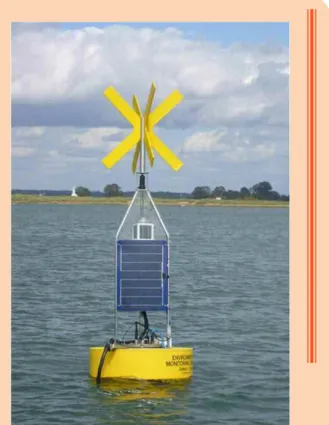
Box 1.4. What is the SIMPATICO
monitoring system?
The SIMPATICO (integrated system for in situ multi-parametric monitoring in coastal area) is an environmental monitoring station owned by CIMA that measures continuously in-situ water quality and currents at the lower Guadiana estuary. The instrumentation consists mainly of a surface buoy (see picture) equipped with a multi-parametric probe and a current-meter. The station provides unique months-long time-series at high frequency (hourly and 15 min) of current velocity (every 80 cm along the water column), water level, temperature, turbidity, dissolved oxygen, salinity, chlorophyll and pH. The data are available publicly at:
http://doi.pangaea.de/10.1594/PANGAEA.845750
Figure 1.7.
(a) water level (m, referred to MSL), and (b) velocity (m/s) variations (blue: along-channel component; green: across-channel component) during one month at the deep channel of the lower Guadiana estuary.
Figure Box 1.4.
The surface buoy of the SIMPATICO system at the lower Guadiana estuary (photograph by E. Garel, 2009).
vice-versa) occurs about 1 hr after high or low water (Figure 1.8). This 1 hr time lag indicates that the tidal wave is a mixture of standing wave and progressive wave (see Box 1.5).
Because the estuarine channel is relatively narrow, the flow is principally parallel to the margins. The cross-channel flow component is weak (generally less than 3 cm/s) compared to the along-channel (or
Box 1.5. What are progressive and
standing waves?
Progressive and standing (or stationary) waves are two types of waves with distinct
characteristics. Progressive waves are those that advance on the sea: a crest, followed by a through, is seen moving along the surface. The amplitude of vertical variations is equal over all points. Maximum water level at a given location occurs at the same time as peak current velocity. On the opposite, standing waves remain at a fixed position, and the amplitude varies from zero (at “node” points) to maximum (at “antinode” points). Standing waves can be seen as the superimposition of two identical progressive waves travelling in opposite directions. This usually happens when one wave is the reflection of the other (see wave reflection in Box 1.6). Maximum water levels for a standing wave occur when the current is null (i.e., when it reverses in direction). In estuaries with semidiurnal tidal variations, the time lag between current and velocity is 0 hr for a purely progressive wave, and about 3 hr for a purely standing wave. However tidal waves at these systems generally consist of mixed waves with intermediate time lag (between 0 and 3 hr).
Figure 1.8.
Example of water level (black, m) and axial velocity (red, m/s) variations during 2 tidal cycles at the lower estuary. The time of maximum tidal stage and slack water are indicated with black and red spots, respectively, to illustrate the time lag (~1 hr) of peak water levels relative to current inversions.
axial) velocity component (Figure 1.7b). Maximum axial velocities are generally observed in the deep channel and near the surface, where they can reach up to 1.4 m/s during the largest spring tides. These velocities may be much higher during periods of large river discharge (see Section 1.4). Considering the average of the flow along the water column, the maximum axial velocity during a tidal cycle is between ~1.3 m/s and 0.4 m/s, depending on the tidal range. It is commonly about 1 m/s at spring tide, and about 0.5 m/s at neap tide (e.g., Figure 1.7).
Laterally, the magnitude of the axial flow is driven by bathymetric variations. The velocity magnitude is weaker at shallower areas where the flow experiences greater bed friction. Around slack water, current reversal (from ebb-directed to flood-directed, and vice-versa) generally occurs first over over shallow areas and
subsequently at the deep channel as the flow has a larger momentum over greater water depths.
1.3.2. Tidal propagation upstream
The mean tidal range is approximately constant along most of the estuary (Figure 1.9, black line).
Significant reduction of the tidal wave height is only observed near the head (upstream of km 60-70) due to truncation of the low water level by sills. At this upstream portion of the estuary, the lowest water level is observed at neap tide rather than at spring tide. This feature distinguishes the tidal river (from km 60-70 until the head) from the tidal estuary located downstream. In detail, some differences in tidal height propagation are observed between spring and neap tides (Figure 1.9, blue and red lines). In particular, along the lower and middle estuary (i.e., between the mouth and ~km 20), the tidal wave is significantly
damped at spring tide but slightly amplified at neap tide. By contrast, the tidal height is similarly amplified at the upper estuary for all tidal ranges. The spring-neap differences in water propagation observed at the lower and middle estuary are due to the non-linear relation between velocity and friction. At spring tide, the bed friction experienced by the flow is much stronger than at neap tide because of larger velocity magnitudes (as friction depends on the square of the velocity). These frictional effects result in tidal damping (see Box 1.6). Bottom resistance is therefore an important factor
influencing the tidal range along the lower and middle estuary, at least at spring tide. By contrast, frictional effects are less at neap tide, and the tide is slightly amplified probably due to morphological convergence at the lower and middle estuary (see Box 1.6). At the upper estuary, the width of the channel changes slowly (see Figure 1.3a). Therefore, the amplification of the tidal wave height due to
morphological convergence should be weaker than at the lower estuary. On the opposite, the largest tidal height amplification is observed at the upper estuary (Figure 1.9). This pattern is due to tidal wave reflection (see Box 1.6), which significantly affects the tidal range upstream of km 30-40.
1.3.3. Tidal asymmetry
When averaged over several months, the difference between ebb and flood duration is small (< 5 min) at the mouth, indicating small distortion. Differences are however observed in the tidal asymmetry between neap and spring tides (Figure 1.10a). At neaps, the flood phase tends to last longer (up to 1hr) than the ebb phase. The opposite is generally observed at springs (longer ebb phase). Furthermore, multiyear observations at the deep channel (from the SIMPATICO System, see Box 1.4) indicate that longer tidal phases are also associated to faster flows (Figure 1.10b). Thus the ebb is longer and faster at spring tide, but it is the flood which is faster and longer at neap tide. The transition between these two asymmetry regimes corresponds very approximately to the tidal range of 2 m. Hence, the lower Guadiana estuary
Figure 1.9.
Tidal range (m) along the Guadiana estuary at spring tide (blue), neap tide (red) and for a mean tide (black). Km 0 corresponds to the southern extremity of the western jetty. The dots indicate the location of the measuring stations.
Figure 1.10.
Tidal asymmetry at the deep channel of the lower estuary: a) difference in flood – ebb duration in hr (y-axis with > 0: flood longer) for ~350 tidal cycles (x-axis), with indication of spring (S) and neap (N) tides; b) peak current velocity (m/s) against tidal range (m) for the ~350 tidal cycles of (a). The tidal range of 2 m is outlined with the dashed red line. The flood phase is longer with faster currents at neap; the ebb phase is longer with faster currents at spring.
Box 1.6. What effects modify the height of a tidal wave when
propagating upstream?
At shallow estuaries, the tidal wave height is affected by the effects of shoaling, damping and reflection as it propagates upstream. Shoaling (or amplification) is due to the gradual
change of the geometry of the system (mainly width, but also depth). This is an important phenomenon in estuaries where the channel width is decreasing significantly towards the head (morphological convergence), such as funnel-shaped coastal plain estuaries. Damping is the reduction of the tidal wave amplitude due to energy loss by friction between the flowing water and the bed. Hence, damping at shallow estuaries is more significant than at deeper systems. The tidal wave height in many estuaries results from the combination of shoaling and damping. If the effect of morphological convergence (i.e., shoaling) is stronger than the effect of friction (i.e., damping), then the wave is amplified; in the opposite case, the wave height is reduced as it propagates upstream. These two opposite effects may
compensate each other, resulting in a constant tidal range along the estuary, as observed in many alluvial estuaries. In this case, the estuary is defined as “ideal” (or “synchronous”). Furthermore, the height of the tidal wave may be, in some cases, affected by reflection. Reflection refers to the propagation of wave opposite to the incoming wave motion due to the presence of a sudden obstacle. The reflecting obstacle might be a step change in water depth, in the case for example of a weir, a sharp bend of the estuarine channel or a vertical wall such as a dam. Partial reflection occurs in the first two cases as part of the wave is transmitted upstream, while the reflection is total in the case of a dam. The tidal range which is observed along the estuary results from the sum (resonance) of the incident wave and transmitted wave. This effect is generally stronger near the reflecting obstacle because the reflected wave is damped by friction as it propagates downstream. For resonance to exist, the period of the tidal wave should be close to the natural period of oscillation of the estuary. For instance, the Bay of Fundy has a natural oscillation period of ~13 hr and displays strong resonance as the semidiurnal tidal wave amplifies upstream as much as 16 m, constituting as such the world’s largest tide.
departs from the typical cases of flood- or ebb-dominated estuaries where longer tidal phases are compensated by lower current velocities (see Box 1.7). The atypical (longer and faster) flows observed at the lower Guadiana estuary are attributed to modifications of the mean character of the flow due to the proximity of the inlet.
Typically, the shape of the tidal wave is increasingly distorted when propagating upstream in relation with reduced bed friction and faster tidal wave velocity around high water (see Box 1.7). Hence, the flood phase tends to be progressively shorter than the ebb one towards the head (Figure 1.11).
Box 1.7. What produce tidal
asymmetry in estuaries?
Tidal asymmetry is due to the interaction of the propagating tidal wave with the bathymetry. As the speed of the tidal wave is controlled by the water depth, high water levels travel faster along the estuary than low water levels. In addition, bed friction is stronger at low tide than at high tide contributing to accelerate the flow at high water in comparison with low water. Because the tide is partially progressive (see Box 1.5), these effects typically result in a flood phase which is shorter than the ebb phase at a fixed location (in the case of a standing wave, these effects are equal during floods and ebbs, and the tide remains symmetrical). To compensate for the shorter flood phase, the tidal velocities are larger during the flood than during the ebb. Estuaries with such a shorter rising tide and larger flood currents are called “flood-dominated”.
“Ebb-dominance” is the opposite deformation (ebb shorter with faster flows) and is generally observed at estuaries with extended tidal marsh areas.
Figure 1.11.
Mean duration of the flood (black) and ebb (red) phases of the tide along the estuary. The dots indicate the location of the measuring stations
In detail, the deformation of the tidal wave is pronounced at spring tide but weak at neap tide (Figure 1.12). This is due to frictional effects related to the difference in tidal range between spring and neap tides (see Box 1.7). Shorter flood phases, in particular at spring tide, suggest flood-dominance. However, scarce velocity measurements indicate that ebb flows are not always weaker than flood ones even when the flood is shorter. Such ebb flow enhancement could be due to
contributions of the freshwater flow component or to the bed slope.
Figure 1.12.
Comparison of the tidal water level variations at km 0 (blue) and km 60 (red) during (a) a neap tidal cycle and (b) a spring tidal cycle.
1.4. Freshwater influence
1.4.1. River discharge into the estuary
The drainage basin of the Guadiana River is the fourth largest on the Iberian Peninsula with an area of 66,960 km2 and a length of 810 km (see also T. Boski, chapter 2 in this book). The Guadiana runoff is closely
related to the regional rainfall patterns due to pronounced shortage of soil and vegetation in the watershed. Strong seasonal and inter-annual variability is featured by prolonged periods of drought alternating episodic floods in winter and spring (Figure 1.13). For example, observations collected between 1947 and 2001 show that from January to March the average freshwater inputs to the estuary ranged from nearly 0 to 4,660 m3/s with a mean of 440 m3/s; from June to August, it ranged from 0 to 50
m3/s with a mean value of 15 m3/s. The maximum historical peak is 11,000 m3/s in 1876, when water level
reached 25 m above its usual height at Mértola. Since February 2002 the flow has been strongly regulated by the large Alqueva dam, located 60 km upstream from the estuary head across the Guadiana River. Some 23 km downstream, the Pedrogão dam forms a 2ndreservoir to pump back the water from the
Alqueva reservoir at times of low demand. Since completion of this dam complex (for simplicity, hereafter referred to as the Alqueva dam), both the magnitude and frequency of floods have been drastically reduced (Figure 1.13).
Figure 1.13.
Daily averaged river discharge (m3/s) into the Guadiana estuary between 1947 and 2017. The red arrow indicates the closure of the Alqueva dam in February 2002.
The present freshwater discharge into the estuary is characterised by long (weeks to months) periods with low values, interrupted by moderate to high inflow events (up to 2,500 m3/s) occurring in the winter
or spring seasons. The low values correspond to the ecological flow for maintaining minimal ecosystem services, which is computed based on rain records at a meteorological station located nearby (Portel). It is typically up to 50 m3/s and should never be less than 3 m3/s. Moderate to high discharge events
correspond to periods of water release from the Alqueva dam and to periods of intense rainfall in the region. During the last 14 years (2002 – 2016), there were only 4 episodes of significant water release from the Alqueva dam, during the first months of 2010, 2011, 2013 and 2014, with discharge roughly between 1,000 and 2,500 m3/s (Figure 1.13). The discharge of rain-induced events is generally weaker, up to ~1,000
1.4.2. Effects of low freshwater inflows into the estuary
When the freshwater inputs to the estuary are low, the salinity front is located at about 25 km from the mouth (near Foz de Odeleite) at low water level, marking the limit between the middle and upper estuary (Figure 1.14). The front moves upstream during flood tide, up to km 40, approximately (near Alcoutim). It should be noted that these features were observed in 2001 and might have been altered due to the present regime of strong flow regulation by the Alqueva dam.
Figure 1.14.
Axial salinity at spring (a, b) and neap (c, d) tides, around high and low water. The river discharge is <10 m3/s for all
cases. The isohaline contour interval is 2 g/kg (except for salinities from 34 to 35 g/kg).
Vertical salinity profiles vary noticeably within the estuary between spring and neap tides (Figure 1.14). At spring tide, the tidal velocities are large and produce boundary turbulences of significant magnitude. As a result of turbulent mixing, the salinity does not change much along the water column, as represented by the vertical isohaline contours in Figures 1.14 (a, b). The estuary is classified as well-mixed under these conditions (see Box 1.8). At neap tide, the turbulence produced by the relatively weaker flow is not sufficient to mix the entire water column. The salinity increases towards the bed, as saltwater is denser thus heavier than freshwater (Figure 1.14 c, d). Under these stratified conditions, ebb flows are promoted near the surface and flood flows are promoted near the bed.
The strength of stratification is affected by tidal velocities (as described above), but also by the water depth. For similar flow magnitude, bed friction and thus mixing is enhanced at shallow areas.
Consequently, significant variations in stratified conditions may be observed both along and across the channel. For instance, in Figure 1.14c and d, the strongest vertical density gradient is located at the deeper portion of the channel axis between km 10 and km 15. It has also been documented that the deep
channel can be partly stratified at the lower estuary, while the bordering shallow areas are well-mixed. These distinct mixing conditions may induce spatial variability in the magnitude and direction of the residual circulation (see section 1.5).
1.4.3. Effects of moderate to high river inflows
A moderate increase in the river inflow enhances the strength of stratification and affects drastically the flow along the entire estuary. This is an essential feature of the Guadiana estuary, due to its constricted morphology, making this estuary very different from other systems with a large watershed such as coastal plain estuaries (where only extreme floods may produce similar effects). For example, highly stratified conditions (characterised by a homogeneous layer of salty water near the bottom, see box 1.8) have been reported at the lower estuary for moderate river discharge of 400 m3/s. In this case, seaward flows are
conditions. Flood flows are restricted to the bottom water layer and are observed during a large part of the tidal cycle to compensate for the long ebb phase at the surface. Hence, downstream- and upstream-oriented flows are commonly observed at the same time near the surface and bottom, respectively. For high discharge events, roughly above 1,000-1,500 m3/s (depending on the tidal range), the entire
estuary is filled up with freshwater during most of the tidal cycle. If the river discharge is not too strong, a salt wedge may propagate upstream during the flood tide due to seawater advection near the bed and reduced mixing by weak flood currents. During the ebb tide, the salt wedge is displaced seaward and riverine characteristics are observed, with a fast unidirectional (downstream) flow of freshwater along the entire water column.
Box 1.8. Estuary classification based on vertical
mixing
A convenient way of classifying estuaries is based on vertical
variations of salinity. This classification considers the mixing between (more dense thus heavier) seawater and (less dense thus lighter) freshwater, and provides important information about the water circulation within the estuary. Four types of estuaries are typically identified: well mixed, weakly stratified (also partly stratified or partially mixed), highly (or strongly) stratified, and salt wedge
estuaries. Well mixed estuaries have typically a large tidal range and a weak river discharge. The mean (tidally-averaged) salinity profiles are uniform along the water column and mean flows are unidirectional with depth. Weakly stratified estuaries have moderate to strong tidal range and weak to moderate river discharge. The mean salinity profile increases more or less regularly from surface to bottom. The mean flow is seaward near the surface and landward near the bed. This water circulation results from the enhancement of density currents and is referred to as the “estuarine (or gravitational) circulation”. Highly stratified estuaries result from weak to moderate tidal range and moderate to large river discharge. The mean vertical salinity profile is relatively constant near the surface (fresher water) and near the bottom (saltier water), the transition occurring across an intermediate layer of water in which the salinity rapidly increases with depth. This stratification remains during the entire tidal cycle. The mean flow features strong surface outflows and weak bottom inflows. Salt wedge estuaries display similar stratification than strongly stratified estuaries, but during the flood tide, only. The stratification results from a large river discharge and weak tidal forcing. Seawater enters the estuary during the flood tide, in the form of a wedge at the bottom. The wedge migrates downstream during the ebb, and might be expelled out of the estuary which is then merely similar to a river, with unidirectional seaward flows and no vertical density gradients (only freshwater). Many systems may evolve from one type to another according to significant changes in the river discharge or to location along the estuary (see also Gomes & Camacho, chapter 3 in this book).
1.5. residual circulation
Residual (also subtidal or net) flows represent the mean water circulation after one or several tidal cycles. They govern the transport of material (e.g., suspended sediment, contaminant, pollutants) along the estuary and the net exchange with the adjacent coastal area, and are therefore of great importance for the health of estuarine ecosystems. The axial residual circulation in estuaries often results from the competition between tidally-induced and density-induced flows (in particular when other forcing agents such as wind or river discharge are unimportant). Thus, this circulation is generally strongly dependent of stratified conditions.
Figure 1.15.
Sketch of the residual circulation at spring (red) and neap (yellow) tides over the deep channel, over the shoals and for the entire cross-section at the lower estuary.
For low river discharge, the overall residual circulation (averaged over the channel width) at the lower Guadiana estuary is upstream at spring tide and downstream at neap tide (Figure 1.15). Albeit a narrow channel, these flow directions vary laterally with the water depth. The residual flows over the shoals are consistent with the channel width-averaged circulation, with inflows at spring tides and outflows at neap tides. By contrast, the tidal asymmetries at the deep channel (described in section 1.3) produce an opposite residual circulation, with inflows at neap tides and outflows at spring tides.
The switch in the net transport direction between spring and neap tides occurs for a tidal range of about 2 m, the average tidal range in the area. For tidal range > 2 m, the estuary is well mixed (see Box 1.8); the residual velocity profile over the deep channel is unidirectional and oriented seaward (green line in Figure 1.16). For a range < 2 m, the deep channel is partly stratified and estuarine circulation develops (see Box 1.8), with a residual flow oriented up-estuary near the bed and down-estuary near the surface (red line in Figure 1.16).
The change in residual water circulation between spring and neap tides is determined (at least partly) by the combination of the Stokes transport and compensating return flow, which varies laterally with the bathymetry (see Box 1.9). The Stokes transport is strong at spring tide over shallow areas and produces an upstream transport of water. At neap tide, the Stokes transport is weak (because variations in water elevation are small), and the return flow is reinforced, producing a downstream residual flow. This flow might be further enhanced by density-induced outflows related to the increased stratification at the deep channel.
Comparison of subtidal water level variations at the mouth and near the head illustrates the fortnightly tide produced by the Stokes transport mechanism (Figure 1.17). At the mouth, water level variations are
Figure 1.16.
Residual velocity profile at the deep channel for low inflow conditions at spring tide (green) and neap tide (red) and for a moderate river discharge of 400 m3/s (blue).
Figure 1.17.
Upper: tidal range at the mouth; Lower: residual water level at the mouth (blue line) and at km 60 upstream (red line).
Box 1.9. What is the Stokes drift in estuaries?
The Stokes drift arises because the discharge of water near to high water is greater than the discharge near low water. This mechanism relates to the progressive component of the (generally mixed) tidal wave (Box 1.5), which induces the transport of more water upstream around high water than downstream around low water (for a purely standing wave, the discharges near high and low water are equal). The Stokes transport is generally stronger over shallow than deep areas because of non-linearity between friction and velocity
(enhanced friction – thus reduced velocity – around low water increases the net difference in water transport between low and high water levels). Likewise, the Stokes transport is also stronger at spring tide when the differences in water levels between high and low tide are larger. The net transport of water upstream produces a gradual increase of the mean water level towards the estuary head resulting in a water level gradient by which a return flow is driven. The interplay between upstream Stokes transport (larger at springs) and downstream return flow (larger at neaps) typically results in water level oscillations at the upper estuary over the spring - neap cycles, referred to as “fortnightly tides”.
small and uncorrelated with the tidal range. By contrast, at upstream locations the water level is generally higher than the mean water level at spring tide, as water is transported towards the estuary head by the Stokes mechanism. At neap tides, the water level decreases and tends to be lower than the mean water level with the transport of water downstream by the return flow. The difference in mean water elevation can be 20 cm (and more) between the mouth and the head (e.g., 01/09/2015 in Figure 1.17).
With increasing freshwater inflows, residual velocity profile at the highly stratified estuary is
unidirectional, oriented downstream, with strong velocities near the surface (Figure 1.16, blue line). The seaward directed residual velocities get larger with increasing river discharge (or with increasing upstream distance from the mouth).
1.6. the transport of sediment
1.6.1. Bedload transport
The bedload sand transport rate is mainly dependent on the tidal current magnitude near the bottom. For low river inflows, maximum velocities at neap tide are too weak to remobilise bed sediment. Significant bedload transport occurs principally at spring tide, when tidal currents are comparatively larger (Figure 1.18). At the lower estuary, the net sand transport is down-estuary due to the tidal
asymmetries reported in section 1.3 (ebb longer and faster at spring tide). Most of the transport occurs at the deep channel where peak velocities are significantly larger than over the shoals. A few near bed measurements also suggest that downstream bedload transport may episodically predominate in the deep channelpredominates at the middle and upper estuary reaches (see section 1.3). In such situations, the deep channel serves as a conduit to export sediment during low inflow conditions. Presently, the estuarine export of sand to the sea is weak, estimated to be about 5,000 m3/yr.
Figure 1.18.
a) Tidal range (m, MSL); b) Tidal (red) and residual (black) bedload transport rate (Qb, m3/m/s); c)
river discharge (m3/s). Significant net bedload
transport occurs at spring tide, only, when the river discharge is low. The transport rate is not enhanced during the periods of increased discharge in Feb. 2008 and Dec. 2009, due to water stratification (discharge < 1,500 m3/s).
For enhanced river inflows, the estuary can be stratified or filled up with freshwater (during part or totality of the tidal cycle) depending on the discharge magnitude and location within the estuary (see section 1.4.3). In the presence of stratification, near bed flows are favoured in the upstream direction by density currents, resulting in long flood phases. There is therefore no significant downstream bedload transport under these stratified conditions (e.g., Figure 1.18). In other words, an increase in river discharge
magnitudes does not necessarily enhance the bedload sand transport towards the sea. Downstream transport rather occurs when freshwater occupies the entire water column during at least a part of the tidal cycle. Such riverine conditions occur for moderate inflows at the middle and upper estuary, supplying bed sediment downstream. At the lower estuary, freshwater is observed for discharge > 1,000 – 1,500 m3/s
dam regulation (Figure 1.13). It has been estimated that the potential for sand export from the estuary to the nearshore has been reduced by 1 or 2 orders of magnitude since the construction of the Alqueva dam.
1.6.2. Suspended sediment
The fine sediment in suspension within the estuary is dominantly composed of phyllosilicates,
represented principally by illite (> 50%), kaolinite and chlorite. Typically, fines are suspended in the water column by tidal currents and deposit at slack water. At spring tide, tidal currents are larger than at neap tides and marginal areas which are usually dry may be inundated. Consequently, the suspended sediment concentration (SSC) varies at a 15 days period (being higher at springs and lower at neaps) when
freshwater inflows are weak. This variability is illustrated by turbidity records – a proxy for SSC - from the SIMPATICO Station (see Box 1.4) at the lower estuary (Figure 1.19). The SSC may also display important variations during a tidal cycle. For example, maximum surface SSC is observed at the end of the ebb (and minimum during the flood) when the seawater is less turbid than estuarine water (such as in Figure 1.19). Occasionally, the seawater can be more turbid than estuarine water leading to maximum SSC values during the flood and minimum values during the ebb.
Figure 1.19.
Turbidity (NTU) records from the SIMPATICO station illustrating variability at the fortnightly and tidal time scales. Periods of ebb and flood tides are in green and blue, respectively.
Figure 1.20.
Axial turbidity (mg/l) at spring (a, b) and neap (c, d) tides, around high and low water. The river discharge is < 10 m3/s for all cases. The filled contours show high turbidity areas.
For low inflows, the SSC ranges usually between less than 10 mg/l at the mouth, up to an estuarine turbidity maximum (ETM) of ~ 500 mg/l located near the haline front, at the middle/upper estuary. At spring tide, the ETM is well expressed and extends along the entire water column (Figure 1.20a, b). At neap tide, it is relatively weaker and restricted to the bed (Figure 1.20c, d). The 2ndETM in Figure 1.20a is
attributed to tributary discharge after an intense rain event. With increasing river flow, the SSC within the estuary might be one order of magnitude larger. For example, a concentration of about 1,000 mg/l was observed near the mouth for a discharge of 2,000 m3/s.
The exchange of suspended sediment between the estuary and the sea is governed by the residual water circulation. Hence, for low river discharge, suspended sediment tends to be imported at springs and exported at neaps (see Section 1.5). Over several weeks, the import and export of fines seem relatively balanced. Significant export takes place during moderate to high river discharge events. The ETM
maintains its position for river discharge up to 250 m3/s (at least) due to increased stratification. For higher
flow, the ETM is displaced downstream and can be expelled out to the shelf. Freshwater plumes of high turbidity are typically observed on the inner shelf during such periods of high river inflows (e.g., Figure 1.21).
Figure 1.21.
Satellite image of the Guadiana estuary during a high river discharge event in December 2001 (source: ISS, NASA).
1.7. Morphodynamics of the ebb delta
The sand deposits that form the Guadiana ebb delta originate from the littoral transport and river export. The littoral transport is eastward in the region (due to the predominance of waves from the Southwest) and estimated about 100,000 m3/yr. The river export is weak during low freshwater inflow conditions
since Alqueva dam closure (about 5,000 m3/yr) but might be one order of magnitude larger in the
occurrence of large flood events (see section 1.6.1).
Before 1972, the (historical) ebb delta was constituted by a broad platform asymmetric towards the East, which included a large sand bank in front of the mouth (the O'Bril bank). Over the course of decades, the bank underwent large morphological changes. Those were accompanied by pronounced modifications in the position and geometry (length, width, water depth) of the inlet channel, making boat access to the estuary hazardous and intricate. To improve navigability, the mouth was stabilised in 1972-74 by a pair of parallel jetties (the eastern jetty being submerged except at low spring tide). This intervention has markedly affected the morphodynamics of the ebb-tidal delta.
In response to jetty construction, the historical delta has been severely eroded under the action of waves. A large part of the eroded material has been transported to the Spanish beaches of Isla Canela, resulting in a significant overall advance of the shoreline. The same mechanism produced accretion of the
Portuguese beach of “Ponta da Areia”, and resulted in the rapid accumulation of sand against the western jetty. A new (modern) delta of smaller dimension has formed off the mouth, characterized by an outer shoal and lateral bars (Figure 1.22). The erosion of the historical delta (and in particular of the O’Bril bank) provided a very large local sand supply which has promoted the rapid development of these
morphological features. At present (2017), the ebb delta is accumulating sand at a reduced pace and migrating seaward at an average rate of about 7 m/yr.
The vertical development of the outer shoal has reduced locally the depth of the navigation channel to less than 3 m (referred to the hydrographic zero; see box 1.3), justifying dredging operations performed in 1986 and 2015. In 2015, a sand volume of 0.063 Mm3was dredged in the channel to reach a minimum
target depth of 3.5 m, for a total cost of 850,000 €. The recovery of the dredged area has been extremely rapid, challenging the efficiency of these dredging operations.
Figure 1.22.
Bathymetry of the ebb delta of the Guadiana estuary in 2014.
1.8. Final remarks
Studies conducted at the Guadiana estuary over the last decades have featured many typical physical processes that have been described at other systems. Yet, various particularities related principally to its (long and narrow) morphology and large watershed should be accounted for to correctly apprehend the dynamics of the Guadiana.
In particular, while estuaries are generally considered as sediment traps due to the infilling of sediment, the Guadiana estuary - as other Rock-Bound Estuaries - exports sediment over time scales of years and more. Weak sediment export associated to low inflows can become substantial for river discharge above 1,000-1,500 m3/s, when the entire estuary is filled up with freshwater for at least a part of the tide. These
high discharge events are however relatively rare and limited in magnitude (up to about 2,500 m3/s)
At most estuaries submitted to average (i.e., non-extreme) conditions, the residual water flows results from the predominance of one physical driver, related for example to the tide or water density
stratification. The magnitude of the residual circulation is in general modulated by the tidal range, being for example weaker (or stronger) at spring tide than at neap tide, but its direction remains constant. By contrast, at the lower Guadiana estuary (and may be upstream), the spring-neap cycle is associated to opposed residual water transport direction during periods of low inflows. These inversions have been rarely described in mesotidal estuaries and suggest a remarkable switching of residual flow drivers at a 15-days period. Some studies have linked this unique behaviour to the variations in stratified conditions observed between spring (well mixed) and neap (partly stratified) tides.
The mean tidal range varies little along most of the Guadiana estuary (from the mouth to ~km 60). This pattern is common at the extensively described large alluvial estuaries, which are then qualified as “ideal”. However, the constant tidal range at alluvial estuaries is produced by a balance between damping (due to friction) and shoaling (due to morphological convergence) of the tidal wave as it propagates upstream (see Box 1.69). By contrast, the constant tidal amplitude along the Guadiana estuary also results from wave resonance, making it different from typical “ideal” systems. As such, the concept of ideal estuary may entail incorrect assumptions when applied to the Guadiana estuary.
Future studies regarding the dynamics of the Guadiana estuary should quantify precisely the water circulation and mixing process along the entire channel for various river flow conditions. This task must account for the variability of the flow across the channel which has been observed (so far) at the lower estuary. Considering its extreme range of stratified conditions (from well-mixed to salt-wedge) and its relatively simple morphology, the Guadiana is an exceptional natural laboratory (with moreover a beautiful natural setting) where these studies should be relevant for a wide range of other systems.
acknowledgements
The author is grateful to D. Moura for the photographs in Figure 2, to J.M.A. Morales for Figures 5 and 6 and to A. Cravo for Figure 21. R. Sampath is acknowledged for providing the estuary width data. Thanks are extended to L. Portela for his time and effort to revise this Chapter.
Consulted bibliography
Cravo, A., Madureira, M., Felicia, H., Rita, F. & Bebianno, M.J., 2006. Impact of outflow from the Guadiana River on the distribution of suspended particulate matter and nutrients in the adjacent coastal zone. Estuarine, Coastal and Shelf Science 70: 63-75.
Dias, J.M.A., Gonzalez, R. & Ferreira, O. 2004. Natural versus anthropic causes in variations of sand export from river basins: an example from the Guadiana river mouth (southwestern Iberia), in: Nawrocki, J. (Ed.), Rapid transgression into semi-enclosed basins. Polish Geological Institute Special Papers, Gdansk, 95-102.
Fortunato, A.B., Oliveira & A., Alves, E.T., 2002. Circulation and salinity intrusion in the Guadiana estuary.
Thalassas 18: 43-65.
Garel, E., Nunes, S., Neto, J.M., Fernandes., R., Neves, R., Marques, J.C. & Ferreira, Ó., 2009. The autonomous Simpatico system for real-time continuous water-quality and current velocity monitoring: examples of application in three Portuguese estuaries. Geo-MarineLetters 29: 331-341.
Garel, E., Pinto, L., Santos & A., Ferreira, Ó., 2009. Tidal and river discharge forcing upon water and sediment circulation at a rock-bound estuary (Guadiana estuary, Portugal). Estuarine, Coastal and Shelf Science 84: 269-281.
Garel, E. & Ferreira, Ó., 2011. Effects of the Alqueva Dam on Sediment Fluxes at the Mouth of the Guadiana estuary. Journal of Coastal Research SI 64, 1505-1509.
Garel, E. & Ferreira, Ó., 2011. Monitoring estuaries using non-permanent stations: practical aspects and data examples. Ocean Dynamics 61: 891-902.
Garel, E. & Ferreira, Ó., 2013. Fortnightly Changes in Water Transport Direction Across the Mouth of a Narrow estuary. Estuaries and Coasts 36: 286-299.
Garel, E. & Sousa, C., Ferreira, Ó., Morales, J.A., 2014. Decadal morphological response of an ebb-tidal delta and down-drift beach to artificial breaching and inlet stabilisation. Geomorphology 216: 13-25. Garel, E. & Ferreira, Ó., 2015. Multi-year high-frequency physical and environmental observations at the
Guadiana estuary. Earth System Science Data 7: 299-309.
Garel, E. & Sousa, C., Ferreira, Ó., 2015. Sand bypass and updrift beach evolution after jetty construction at an ebb-tidal delta. Estuarine, Coastal and Shelf Science 167 (Part A): 4-13.
Garel, E. & D’Alimonte, D., 2017. Continuous river discharge monitoring with bottom-mounted current profilers at narrow tidal estuaries. Continental Shelf Research 133: 1-12.
Gonzalez, R., Dias, J.M.A. & Ferreira, Ó., 2001. Recent rapid evolution of the Guadiana estuary mouth (southwestern Iberian Peninsula) Journal of Coastal Research Proceedings of International Coastal Symposium 2000, 516-527.
Lobo, J., Plaza, F., Gonzáles, R., Dias, J., Kapsimalis, V., Mendes, I. & Rio, V., 2004. Estimations of bedload sediment transport in the Guadiana estuary (SW Iberian Peninsula) during low river discharge periods. Journal of Coastal Research, Special Issue 41: 12-26.
Machado, A., Rocha, F., Gomes, C. & Dias, J., 2007. Distribution and Composition of Suspended Particulate Matter in Guadiana estuary (Southwestern Iberian Peninsula). Journal of Coastal Research 50: 1040 -1045.
Morales, J.A., 1997.Evolution and facies architecture of the mesotidal Guadiana River delta (S.W. Spain-Portugal). Marine Geology 138: 127-148.
Morales, J.A., Delgado, I. & Gutierrez-Mas, J.M., 2006. Sedimentary characterization of bed types along the Guadiana estuary (SW Europe) before the construction of the Alqueva dam. Estuarine, Coastal and
Shelf Science 70: 117-131.
Portela, L., 2006. Sediment delivery from the Guadiana estuary to the coastal ocean. Journal of Coastal