Musical pattern extraction using genetic algorithms

Musical Pattern Extraction Using Genetic Algorithms

1 _{Departamento de Engenharia Informática da Escola Superior Tecnologia e Gestão de Leiria;} Morro do Lena, Alto Vieiro, 2401-951 - Leiria, Portugal

2 _{Centro de Informática e Sistemas da Universidade de Coimbra;} Polo II, Pinhal de Marrocos, 3030 - Coimbra, Portugal

{grilo, amilcar}@dei.uc.pt

Abstract. This paper describes a research work in which we study the

possibility of applying genetic algorithms to the extraction of musical patterns in monophonic musical pieces. Each individual in the population represents a possible segmentation of the piece being analysed. The goal is to find a segmentation that allows the identification of the most significant patterns of the piece. In order to calculate an individual’s fitness, all its segments are compared among each other. The bigger the area occupied by similar segments the better the quality of the segmentation.

1

Introduction

In artificial intelligence, it is common to name the process of identifying the most meaningful patterns occurring in some piece of data as pattern extraction. An important branch of this investigation area is dedicated to the problem of identifying the most meaningful patterns in data that can be represented as strings of symbols. This is a problem of great relevance in areas like molecular biology, finance or music. In the particular case of music, the identification of these patterns is crucial for tasks like, for example, analysis, interactive on-line composition or music retrieval [1]. In previous work done in this area ([2], [3], [4]), the musical piece to be analysed can be almost exhaustively scanned, so that all the existing patterns are identified. After that, some criteria are applied so that the most meaningful patterns can be identified. While this may be an effective procedure, we think that it is reasonable to investigate the possibility of identifying the most meaningful patterns existing in one musical piece without searching the entire space of its segments.

This paper describes a research work in which we study the application of genetic algorithms to the extraction of musical patterns in monophonic musical pieces. The two main reasons for choosing genetic algorithms to this type of problems are: the search capacity already demonstrated by these algorithms in very complex problems; the possibility of representing individuals as possible segmentations of the piece being analysed. This way, if we guide the search such that segmentations with the most meaningful patterns are favoured, at the end it will not be necessary to do extra processing. Since until now we have been more concerned with the question of “how can this be done?” and with “does it solve the problem?” than with “how fast it is”, this paper will not cover aspects related to time performance.

EMPE (Evolutionary Musical Pattern Extractor). In Section 3 we show the results obtained in some experiments that we have done. Finally, in Section 4 we draw some conclusions and indicate some future steps in our research.

2

EMPE Description

EMPE uses a genetic algorithm to discover the most significant patterns existing in a musical piece. It receives the piece to be analysed as an argument and returns a segmentation of that piece.

2.1 The Genetic Algorithm

Genetic algorithms are parallel and stochastic search algorithms inspired by the evolution theory and molecular biology, which allow the evolution of a set of potential solutions to a problem. In our approach, we use is a typical genetic algorithm, although with some changes. It starts by randomly creating an initial population P(0) of size n of potential solutions to the problem (each one represents a segmentation of the piece being analysed; see Section 2.2). Then, it evaluates this population using a fitness function that returns a value for each individual indicating its quality as a solution to the problem.

After these two steps it proceedsiteratively while a stop condition is not met. In each iteration, the first step consists of the creation of a new population P1(t), also of size n, by stochastically selecting the best individuals from P(t), the current population. Among the several existing selection methods, we use the tournament selection method [5], with tournament size of 5. After the selection step, a new population P2(t) is created by stochastically applying genetic operators to the individuals of P1(t). The genetic operators we use are classical two-point crossover and classical mutation [5]. After the application of genetic operators we introduce another step that, while not being a new one, doesn’t make part of typical genetic algorithms. It consists of the application of another type of operators, usually called learning operators [6], to some individuals of P2(t). This step is inspired by the fact that the performance of biological organisms can be improved during their lifetime through learning processes. In artificial systems, some common differences between genetic and learning operators are: genetic operators have a predefined probability of being applied to any individual, while learning operators are usually applied only to a small randomly chosen set of individuals; learning operators, differently from genetic operators, are usually deterministic and are sequentially and repeatedly applied to each chosen individual during a fixed number of iterations or until their application stops improving the individual’s fitness. The learning operators used in our algorithm will be described in section 2.4.

In the last step of the cycle, the modified P2(t) becomes P(t+1), whose individuals are then evaluated using the already mentioned fitness function. Finally, after the search process is terminated the learning operators are applied to the best individual found, so that some last improvements can be made.

2.2 Individual’s Representation

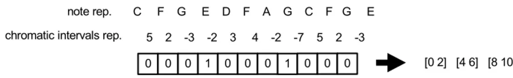
it consists on a sequence of segments in which the piece can be divided. Fig. 1 illustrates how individuals are represented and how they must be interpreted.

5 2 -3 -2 3 4 -2 -7 5 2 -3 C F G E D F A G C F G E

1

0 0 0 1 0 0 0 0 0 0 note rep.

chromatic intervals rep.

[0 2] [4 6] [8 10]

Fig. 1. A sequence of chromatic intervals and an individual representing a segmentation of it As we can see in this figure, each individual consists of a binary string. All individuals of the population have the same length, equal to the number of intervals of the piece to be analysed (although in Fig.2 we only show information relative to pitch, we actually represent musical pieces as sequences of tuples <chromatic_interval, duration_ratio>). The i-th digit of the binary string corresponds to the i-th interval of the piece. Segments simply correspond to “0” sequences, being the “1”s to represent intervals that, being between segments, do not belong to any. Following this interpretation, the individual of Fig. 1 corresponds to the interval segments sequence “{5, 2, -3}, {3, 4, -2} {5, 2, -3}”, equivalent to the note segments sequence “{C, F, G, E}, {D, F, A, G}, {C, F, G, E}”.

Due to practical reasons, before the learning operators application step, we convert individuals into a representation of the type “[lo ro] ... [ln rn]”, where [li ri] stands for

the i-th segment of the piece, and li and ri represent, respectively, the left and right

limits of that segment. This type of representation, besides being a more understandable one, has the advantage of allowing an easier access to segment limits, which among other things, facilitates the evaluation process. Thus, in practice we have two types of representation: one we refer to as the genotype, on which genetic operators are applied, and another we refer to as the phenotype, into which individuals are converted before the learning operators application step. In order to facilitate the reading, in the rest of the paper we will use preferably the phenotype representation instead of the genotype one.

In EMPE, as we allow the user to define upper and lower limits to segments’ length through, respectively, parameters min_seg_len and max_seg_len, it may happen that the application of genetic operators generates individuals with segments that violate these limits. In order to correct these situations, all individuals resulting from the application of genetic operators are submitted to the following correction procedure: if a too small segment occurs, concatenate it with the next segment (this is done easily by changing the “1” between the two segments by a “0”); if a too big segment occurs, divide it in two equal length segments.

2.3 Fitness Evaluation

Individuals, as described in the previous section, do not say anything about which segments are patterns. This information is attached to each individual during the evaluation process in the form of relations between segments, as we will now see. The fitness of an individual is calculated by comparing all its segments among each other. If the distance between two segments is less than a given value, they are

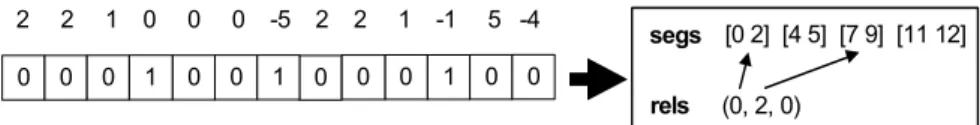
considered similar and a relation between them is created. If this is not the case, no relation is created and the two segments are not considered as similar. Every time a relation is created, the difference value between the two segments is attached to it. In Fig. 2 we show an individual and the relations that are created as a result of this process (in this case, just one). Each relation is represented by a structure (seg1_ pos,

seg2_ pos, dif), where seg1_ pos and seg2_ pos are the ordinal positions of the two

segments (we consider that the first segment’s position is 0) and dif is the difference between them. Although, from the genetic algorithm point of view, relations aren’t part of individuals, it is obvious that this information is essential for the appreciation of the merit each individual has. Thus, whenever possible, in the rest of the paper individuals will be followed by the relations existing between their segments.

segs 2 2 1 0 0 0 -5 2 2 1 -1 5 -4 0 0 0 0 1 0 0 1 0 0 1 [0 2] [4 5] [7 9] [11 12] 0 0 (0, 2, 0) rels

Fig. 2. An individual representing a segmentation of a musical excerpt and the relations created

as a result of the evaluation process

The goal of the system is to find an individual for which the sum of the length of the segments participating in relations is the maximum possible and for which de sum of the differences attached to all the created relations is the minimum possible. Stated another way, the goal is to find an individual that maximizes the following function

∑

∑

×

+

×

=

b

area

s

rel

d

a

x

f

)

(

)

(

)

(

where x is the individual to be evaluated, a is a negative constant, b is a positive constant, m is the number of relations created as a consequence of the segment comparison process, d(reli) is the difference attached to relation reli calculated with

the Wagner-Ficher algorithm [7], n is the number of segments of x, and

     + = not if , 0 relation, one least at of part makes segment if , 1 ) ( i i i i s - l r s area

is the length of each segment participating in at least one relation (the length of each segment is summed only once, even if it participates in more than one relation). The Wagner-Ficher algorithm measures the distance between two strings by the number of operations of insertion, deletion and substitution needed to transform one into the other. The difference value between two segments, under which they are considered similar, was defined empirically as 5, if the smaller segment has length greater than 20, and as ¼th of the smaller segment length, if not. We admit that more work is needed to choose the appropriate values.

Besides the difference between two segments, another aspect that can prevent the creation of a relation between them is their length. Actually, we allow the definition of a minimum value to the segments length – which we call min_pat_len – under which a segment cannot be considered similar to any other segment. This doesn’t mean, however, that segments with a length less than min_pat_len cannot exist (the

parameters that actually bound segments length are min_seg_len and max_seg_len). The existence of the min_pat_len parameter allows us to define that, for example, in the first segmentation of the piece being analysed, only the bigger patterns can be identified, although small rests, which are segments that don’t participate in any relation, can coexist with these patterns in the segmentation.

A last word about evaluation: in the present version of the system, segments are only compared in their original form. This does not mean, however, that they cannot be also compared, for example, in their retrograde or inverted form. In fact, this will be one of the next steps we will take in improving the system.

2.4 Learning Operators

In the learning operators application step, four operators are applied to a small randomly chosen set of individuals. These operators are applied iteratively to each chosen individual until it is not possible to improve its fitness. At the end of each cycle the correction procedure described above is applied in order to correct possible invalid situations, but now at the phenotype level. This operation can, however, deteriorate the individual’s fitness to a level worst than it had before the learning process. Consequently, the modifications done by the operators and the correction procedure only acquire a definitive character if at the end of the process an effective improvement is achieved. If this is the case, the individual’s genotype is updated in order to reflect the modifications done at the phenotype level. We will now describe the four operators used in the learning process.

The first operator does the same thing to all limits between segments: first, it tries to shift the limit to the left the more units it can, which means that it stops once this implies a decrease in the individual’s fitness. When this happens, it tries the same thing, but now to the right. Fig. 3 illustrates the shifting in one unit to the left of the limit between the first and the second segments of an individual.

[0 4] [6 7] [9 10] [12 13] [15 16] [0 3] [5 7] [9 10] [12 13] [15 16] Fig. 3. First learning operator application example

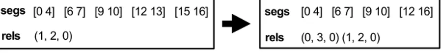
The second operator consists just in concatenating all the individual’s consecutive rests. This operator, as the one we will describe next, was initially conceived with the single purpose of simplifying individuals’ structure. However, its application can also cause an improvement in the individual’s fitness since it is possible that it leads to the creation of new relations in which the new segments participate. Fig. 4 illustrates this situation. 2 2 1 -1 -4 9 2 -2 0 2 -2 -9 2 2 1 -1 -4 [0 4] [6 7] [9 10] [12 13] [15 16] segs (1, 2, 0) rels [0 4] [6 7] [9 10] [12 16] segs (0, 3, 0) (1, 2, 0) rels

(Segments [12 13] and [15 16] are two consecutive rests)

The third operator is better described through an example. Consider the musical excerpt of Fig. 5, which has an AXA structure. The individual allows the identification of all recurrent existing material, but it has a clearly more complicated structure than needed (ABCXABC). The purpose of this operator consists on the detection of these situations and on the simplification of individuals if this does not imply a fitness decrease. It can also be viewed as a bias for segmentations with longer patterns. Thus, although the fitness function does not state any preference for longer patterns this preference exists and is expressed through this operator.

2 2 1 4 2 -2 -4 -3 -2 4 -2 -2 2 2 1 4 2 -2 -4 -3 C D E F A B A F D C E D C D E F A B A F D [0 1] [3 4] [6 7] [9 10] [12 13] [15 16] [18 19] segs (0, 4, 0) (1, 5, 0) (2, 6, 0) rels [0 7] [9 10] [12 19] segs (0, 2, 0) rels A X A

Fig. 5. Third learning operator application example

The fourth operator is similar to the first one, but it operates simultaneously on the limits of segments that together participate in one relation. Consider, for example, that there exists a relation between segments [lx rx] and [ly ry]. This operator starts by

trying do shift the left limit of both segments to the left, resulting in the new segments [lx-1 rx] and [ly-1 ry] (these modifications imply that the limits of adjacent segments

are also modified). This procedure is repeated while it does not decrease the individual’s fitness. When this happens, the operator tries to shift left limits to the right the more positions it can. After left limits are treated, the same procedure is applied to the segments’ right limits, but now, first to the right and then to the left. 2.5 Further Segmentations

It is consensual that almost all musical pieces have a hierarchical structure. This means that they are composed of bigger related segments that are also decomposable into smaller ones. In EMPE, further segmentations are done by first choosing some of the segments identified in the previous segmentation and then applying the same segmentation process to a “new musical piece” composed by these segments.

Although segment classification is not a central goal of our work, the problem of deciding which segments must be chosen to make part of the “new piece” to be analysed can be seen as the one of choosing the most representative segment - the prototype - of each segment class existing in the musical piece being analysed. The classification algorithm we used, which we will not describe in this paper due to lack of space, is rather rudimentary, being one of the main aspects we must improve in the future. One of its characteristics is that similarity relations between segments are considered as transitive, which is not true. This means that, if segment s1 is similar to

s2, and s2 to s3, then all the three will belong to the same class, even if s1 and s3 are not

in none of them a class was created to which two dissimilar segments belonged. After the classification process, we must decide which of the segments of each class is its prototype. This decision is taken in the following way: if the class has just one segment, then that segment is its prototype; if it has two segments, choose the smaller of the two segments; if the class has more than two segments, its prototype is the segment to which the sum of the differences between it and the other segments of the class is smaller.

The “new piece“ to be analysed is created juxtaposing the chosen segments by the order they appear in the original piece. Between each two segments a special interval is inserted with the purpose of preventing, in the next segmentation, the creation of segments that are not sub-segments of the previously identified ones. This is achieved by placing a 1 in all individuals’ genotype positions corresponding to special intervals and by prohibiting genetic and learning operators from modifying them.

3

Experimentation

In this section, we show the results obtained after some experiments done with the troubadour songs «Maria muoter reinû maît» (Fig. 6) and «Kalenda Maya» (Fig. 9), used by Ruwet in [8] to exemplify his analysis procedure. In these figures, we also show what segments this author identified. We have done 30 runs for each piece and, in each run, we used populations of 100 individuals evolving during 100 generations (the termination criterion is the number of generations since it is impossible to know, in advance, what is the fitness value corresponding to the best segmentation). The probability of applying crossover and mutation operators was defined, respectively, as 70% and 1%. In each generation, only one individual was submitted to the learning process. Values used for weights a and b of the fitness function were, respectively, -2 and 1. Parameters max_seg_len and min_seg_len were defined, respectively, as half the length of the piece and 2. Finally, parameter min_pat_len was defined as 10% of the length of the piece in the first segmentation and 2 in the second.

3.1 «Maria muoter reinû maît»

Fig. 6. «Maria muoter reinû maît»

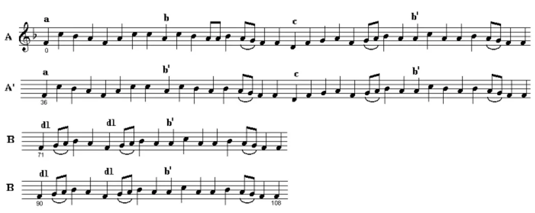
30 runs have a structure identical to the one depicted in Fig. 7, which corresponds to the first segmentation done by Ruwet. We can, thus, say that EMPE has no difficulty in discovering the higher-level structure of this piece.

0[0 34] 1[36 69] 2[71 88] 3[90 107] segs

(0, 1, 5) (2, 3, 0)

rels

A A' B B

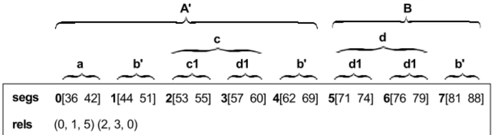
Fig. 7. Best individuals generated in the first segmentation of «Maria muoter reinû maît» The second segmentation was done using an interval sequence constructed from segments identified in the first segmentation. This sequence is composed by segments [36 39] and [71 88] (respectively, segments A’ and B) by this order. Individuals equal to the one depicted in Fig. 8, which nearly correspond to the second segmentation done by Ruwet, were generated in 21 of the 30 runs. The only differences are that segments c and d are both divided in two. However, it is only possible to identify the three occurrences of segment d1 by dividing them.

0[36 42] 1[44 51] 2[53 55] 3[57 60] 4[62 69] 5[71 74] 6[76 79] 7[81 88] segs (0, 1, 5) (2, 3, 0) rels a b' c1 d1 b' d1 d1 b' c d A' B

Fig. 8. Best individuals generated in the second segmentation of «Maria muoter reinû maît» 3.2 «Kalenda Maya»

Fig. 9. «Kalenda Maya»

In the first segmentation of this piece, 20 runs resulted in individuals with the same structure of the one in Fig. 10.

0[0 20] 1[22 42] 2[44 52] 3[54 62] 4[64 72] 5[74 77] 6[79 87] 7[89 94] segs

(0, 1, 0) ((2, 3, 2) (4, 6, 0)

rels

A A B B'

Fig. 10. Best individuals generated in the first segmentation of «Kalenda Maya» As is possible to confirm in this figure, these individuals’ first four segments correspond to the first four segments identified by Ruwet. In order to explain the configuration of these individuals’ last four segments we must first turn our attention into the two segments Ruwet identifies as D and D’. The difference between them, calculated with the Wagner-Ficher algorithm, is equal to 6, which is greater than ¼th of the length of segment D, the smaller of the two segments. This means that, even if an individual had two segments corresponding to segments D and D’, no relation would be created between them during the evaluation process.

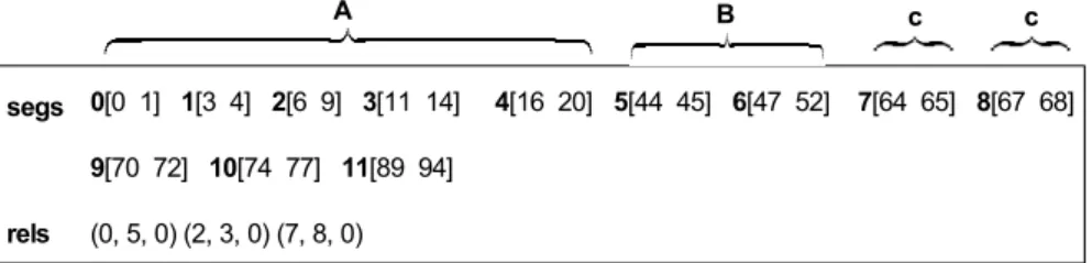
Given the impossibility of associating segment D and D’ through a similarity relation, what does the genetic algorithm? Following the fitness function, it tries to find segments that lead to a bigger portion of covered area with the minimum possible differences between related segments. In order to achieve this, after the first four segments, it divides the rest of the piece in another four segments, two of which are equal (segments 4 and 6 in Fig. 10). These two segments, constituted by two occurrences of segment c plus the common beginning of segments D and D’, are, after the two occurrences of segment A, the two bigger identical segments of the piece. This way of doing things is, in fact, consistent with Ruwet’s analysis procedure: “first try to identify the bigger identical segments existing in the piece”. In the second segmentation of this piece, the interval sequence that was analysed was composed by segments [0 20], [44 52], [64 73], [75 77] and [71 88] by this order. Fig. 11 depicts the structure of the 18 best individuals generated in the 30 runs done. These individuals, besides the two occurrences of segment c, allow the identification of the similarity between the beginning of segments A and B/B’ (segments 0 and 5 in the figure), and the similarity between two sub-segments of A (segments 2 and 3).

segs (0, 5, 0) (2, 3, 0) (7, 8, 0) rels 0[0 1] 1[3 4] 2[6 9] 3[11 14] 4[16 20] 5[44 45] 6[47 52] 7[64 65] 8[67 68] 9[70 72] 10[74 77] 11[89 94] c c A B

Fig. 11. Best individuals generated in the second segmentation of «Kalenda Maya»

4

Conclusions and Future Work

In this paper we have presented a genetic algorithms based approach to musical pattern extraction. In the first phase of this research work we have been more engaged with the question of how this type of algorithms can be used to effectively solve the

problem without worrying about complexity issues. The experiments we have done allow us to think that, in fact, this approach is a viable one (besides «Maria muoter reinû maît» and «Kalenda Maya», we have done experiments with some others pieces as, for example, Debussy’s «Syrinx», with also good results).

Our future work will comprise two types of tasks: some in which the goal will be to increase the quality of the generated segmentations, as well as the probability of generating them, and some in which the goal will be to study and, if possible, reduce the algorithm’s complexity (each run for the first segmentation of the two pieces used in this paper took approximately 0.4 seconds in a AMD Athlon XP 1.54 GHz). Some ideas for the first set of tasks are: the utilization of more music oriented distance measures such as the ones described in [2] or [9]; the comparison of segments in their retrograde and inverse form; the utilization of a better classification algorithm. In what concerns to complexity, it can be reduced if we avoid the comparison of two segments more than once. This may happen because it is almost certain that, during the search process, two or more individuals will have some common segments. We think that a data structure similar to the one used in [2] may help avoiding this repetition. The challenge with this method will be to maintain space complexity to reasonable levels.

References

1. Rolland, P.Y, Ganascia, J.G.: Musical Pattern Extraction and Similarity Assessment. In E. M. Miranda (Ed.), Readings in Music and Artificial Intelligence, Harwood Academic (2000) 115-144

2. Rolland, P.Y.: Discovering Patterns in Musical Sequences. In Journal of New Music Research, 28, nº 4 (1999) 334-350

3. Cambouropoulos, E.: Towards a General Computational Theory of Musical Structure. PhD Thesis, University of Edinburgh (1998)

4. Meredith, D., Wiggins, G. A., Lemström, K.: Pattern Induction and Matching in Polyphonic Music and Other Multi-dimensional Datasets. Proceedings of the 5th World Multi-Conference on Systemics, Cybernetics and Informatics (SCI2001), Volume X (2001) 61-66

5. Mitchell, M.: An Introduction to Genetic Algorithms, MIT Press (1996)

6. Pereira, F.: Estudo das Interacções entre Evolução e Aprendizagem em Ambientes de Computação Evolucionária. PhD Thesis, Universidade de Coimbra (2002) 7. Stephen, G.: String Search. Technical Report, School of Electronic Engineering

Science, University College of North Wales (1992)

8. Ruwet, N.: Langage, Musique, Poésie. Editions du Seuil, Paris (1972)

9. Perttu, S.: Combinatorial Pattern Matching in Musical Sequences. Master´s Thesis, University of Helsinki, Series of Publications, C-2000-38 (2000)