1
Hydrodynamic changes imposed by tidal energy converters on extracting energy 1
on a real case scenario 2
Pacheco, A.1*, Ferreira, Ó.1
3
1CIMA/Universidade do Algarve, Edifício 7, Campus de Gambelas Faro, 8005-139, Portugal, ampacheco@ualg.pt, 4 oferreir@ualg.pt 5 6 Abstract 7
The development on tidal turbine technology is ongoing with focus on several aspects,
8
including hydrodynamics, operation and environment. Before considering an area for
9
exploitation, tidal energy resource assessments in pre-feasibility energy extraction areas
10
must include the relevant characteristics of the device to be used. The present paper uses
11
the momentum source approach to represent a floatable tidal energy converter (TECs) in
12
a coastal hydro-morphodynamic model and to perform model simulations utilising
13
different TEC array schemes by quantifying the aggregated drag coefficient of the
14
device array. Simulations for one-month periods with nested models were performed to
15
evaluate the hydrodynamic impacts of energy extraction using as output parameters the
16
reduction in velocity and water-level variation differences against a no-extraction
17
scenario. The case study focuses on representing the deployment of floatable E35
18
Evopod TECs in Sanda Sound (South Kintyre, Argyll, Scotland). The range in power
19
output values from the simulations clearly reflects the importance of choosing the
20
location of the array, as slight changes in the location (of <1 km) can approximately
21
double the potential power output. However, the doubling the installed capacity of
22
TECs doubles the mean velocity deficit and water-level differences in the area
23
surrounding the extraction point. These differences are amplified by a maximum factor
24
of 4 during peak flood/ebb during spring tides. In the simulations, the drag coefficient is
25
set to be constant, which represents a fixed operational state of the turbine, and is a
26
limitation of coastal models of this type that cannot presently be solved. Nevertheless,
27
the nesting of models with different resolutions, as presented in this paper, makes it
28
possible to achieve continuous improvements in the accuracy of the quantification of
29
momentum loss by representing turbine characteristics close to the scale of the turbine.
30 31
Keywords: Tidal energy; Tidal energy converters; Floatable tidal turbines; 32
Hydrodynamic modelling; Sanda Sound, Scotland.
2 1. Introduction
34
The hydrokinetic energy that can be extracted from tidal currents is one of the most
35
promising renewable energy sources [1]. Tidal energy extraction is very site specific,
36
that is, the methods for determining the limits of and potential for energy extraction
37
from a channel differ from site to site. Although the effects of removing energy may not
38
be detectable when one or even ten tidal turbines are concerned, extracting tidal energy
39
at commercial scales can potentially have several impacts on the environment, including
40
a reduction in tidal amplitude, disruptions to flow patterns and concomitant changes in
41
the transportation and deposition of sediments, changes in the population distributions
42
and dynamics of marine organisms, modifications to water quality and marine habitats,
43
increases in ambient noise, and greater levels of mixing in systems in which salinity and
44
temperature gradients are well defined [2–7]. Disruptions to flow patterns may also
45
have consequences for the downdrift energy extraction potential, endangering
46
implementation schemes and their efficiency; for example, the efficiency of a Tidal
47
Energy Converter (TEC) positioned in the wake of another device within TEC array
48
schemes.
49
An understanding of the hydrodynamic shifts induced by TEC devices can be obtained
50
through the use of numerical modelling techniques, calibrated using databases for
51
different test case sites. When modelling the flow across turbines, a decision has to be
52
made about how the properties of TECs should be represented in the coastal model, that
53
is, how the drag forces associated with power extraction are modelled. The
54
representation of those forces aims to “upscale” the effects of the detailed flow and
55
turbulence around a simplified turbine to give a coarse representation of the
56
hydrodynamic forces acting on a turbine or on a group of turbines [8]. In the open
57
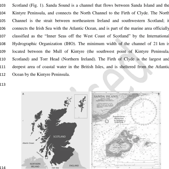
source Delft3D model, this can be effectively performed using porous plates by analogy
58
with the actuator disc theory. The data needed for applying this approach require the
59
determination of a momentum loss term able to represent the extraction of energy from
60
the free flow. Ideally, this loss term should be determined by analysing the turbulence
61
scales and velocity profile distortion under different flow conditions while operating
62
TECs in real conditions. However, because the availability of data on operating TECs in
63
real conditions is scarce, the momentum loss term is calculated based on TEC prototype
64
characteristics, physical assumptions, and/or data collected from testing scale models in
65
physical tanks. Prior to adding the momentum loss term into the modelling equations
3
and evaluating different energy extraction scenarios based on simulations, the numerical
67
models first need to reproduce the hydro-morphodynamic characteristics of the area of
68
interest.
69
This paper presents the methods for setting up the Delft3D model at Sanda Sound,
70
South Kintyre Peninsula (Argyll, Scotland) to gain realistic insights into the
71
hydrodynamic impacts of energy extraction in confined channels and to consider
72
different solutions for effectively simulating energy extraction with reference to the
73
installation of an array of devices (E35 Evopods) within the study area. The paper
74
explains the modelling set-up, the calibration factors used, and the validation procedures
75
adopted both before and after incorporating turbine effects. The turbine characteristics
76
were obtained using drag data from prototype testing in both physical tanks and real
77
conditions. These values were used for determining the momentum loss term induced
78
by the energy extraction, which was then implemented on the numerical mesh via
79
porous plates and using appropriate scaling factors. This procedure allowed the
80
momentum loss term derived from the energy extraction of an idealised array scheme to
81
be determined and simulations to evaluate the potential impacts of energy extraction on
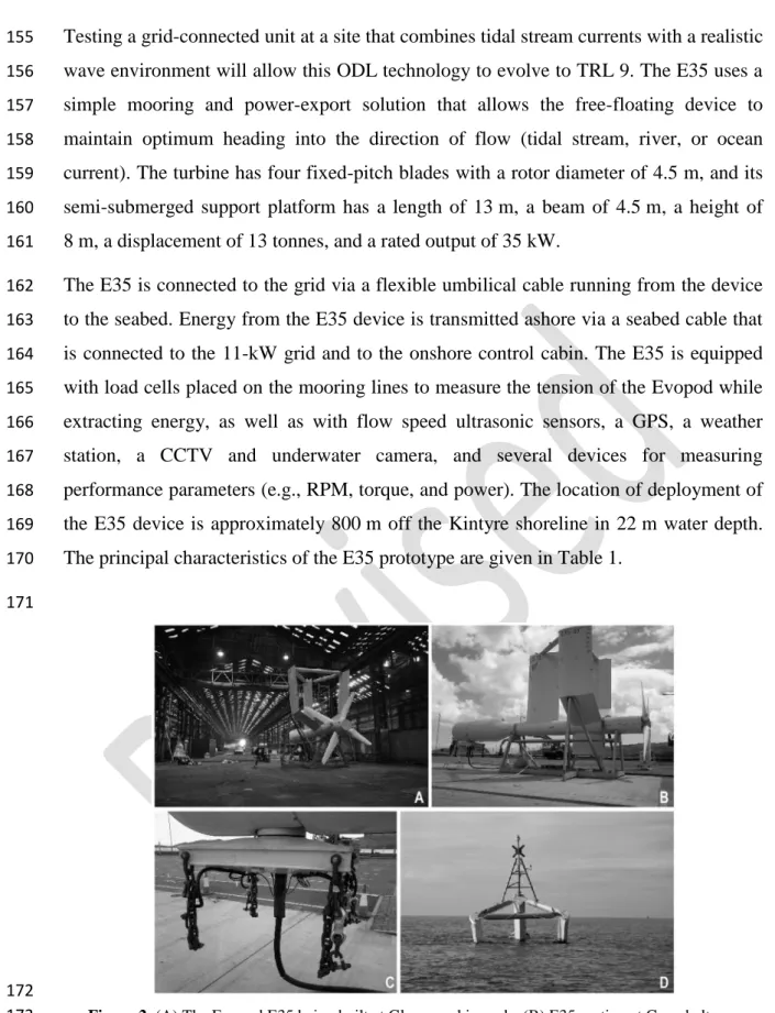
82
flow patterns to be performed.
83
The novelty of the present paper can be stressed by two main points: (1) this is the first
84
paper trying to model floatable tidal devices (e.g. such as the Evopod) on a numerical
85
modelling using the aggregate drag approach to reproduce the effects of energy
86
extraction by an array scheme. The attempt relates directly to the local 1MW project
87
that is predicted to future be implemented at Sanda Sound; and (2) the methodology
88
used to achieve the proposed goals is focused on the use of coupled nested models using
89
Delft3D Dashboard, an approach that can be easily implemented elsewhere. Although
90
direct comparisons with experimental data will be carried on soon as the prototype is
91
fully functional on the water, the present paper addresses the challenges of setting up a
92
model on a remote coastline such as Sanda Sound making the best use of the available
93
information (e.g. coupling available bathymetric and hydrodynamic data, existing data
94
on Evopod testing in the Newcastle wave-current-wind tank and on the real case
95
scenario of Strangford Lough). Those tests allowed determining the drag forces
96
associated with energy extraction from the free flow, which complemented the available
97
data on the characteristics of the 1:4 Evopod prototype (E35 kW).
98 99
4 2. Study case
100
2.1. Site characteristics 101
The study site is Sanda Sound, which is located off the Mull of Kintyre in southwest
102
Scotland (Fig. 1). Sanda Sound is a channel that flows between Sanda Island and the
103
Kintyre Peninsula, and connects the North Channel to the Firth of Clyde. The North
104
Channel is the strait between northeastern Ireland and southwestern Scotland; it
105
connects the Irish Sea with the Atlantic Ocean, and is part of the marine area officially
106
classified as the “Inner Seas off the West Coast of Scotland” by the International
107
Hydrographic Organization (IHO). The minimum width of the channel of 21 km is
108
located between the Mull of Kintyre (the southwest point of Kintyre Peninsula,
109
Scotland) and Torr Head (Northern Ireland). The Firth of Clyde is the largest and
110
deepest area of coastal water in the British Isles, and is sheltered from the Atlantic
111
Ocean by the Kintyre Peninsula.
112 113
114
Figure 1. (A) Map of Scotland with small box (bottom left) depicting the location of the test site, Sanda 115
Sound; (B) Admiralty Chart 2126 marking the location of the Evopod E35 mooring (circle)
116 117
2.2. Oceanographic setting 118
Scotland’s location in the northern part of the British Isles and the steep bathymetry of
119
the continental slope together act as a barrier between the oceanic regions and the shelf
120
sea systems, reducing the amount of water that is able to move from the deeper waters
121
of the North Atlantic into the shallower waters of the Scottish continental shelf.
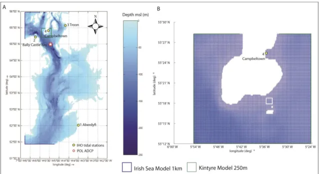
5
Scotland has a maritime climate that is strongly influenced by the oceanic waters of the
123
North Atlantic and the prevailing southwesterly winds. As these winds blow over the
124
regions of the North Atlantic, warmed by the North Atlantic Current, they pick up heat
125
that gives Scotland a relatively mild, wet climate considering its latitude [9].
126
The wave climate of Scotland is influenced mainly by conditions in the North Atlantic
127
Ocean, where the fetch is sufficiently long to establish large, regular waves (i.e., swell)
128
[10]. The north and west of Scotland (the Hebrides, Orkney Islands, and Shetland
129
Islands) are most exposed to these conditions [11,12]. Wave heights are greatest in the
130
most exposed waters of the north and west, and decrease markedly into the North Sea
131
and southwards from there into both the Irish Sea and the English Channel [13]. Within
132
the Irish Sea, the waves tend to be locally generated, have fairly short periods (50-yr
133
mean values in the order of 10 s within the Irish Sea and 15 s at its outer entrances), and
134
are relatively large (50-yr significant wave heights ranging from 8 m within the Irish
135
Sea to 12 m at its entrances) [14]. Sanda Sound is protected from NW waves because of
136
Kintyre Peninsula, but is relatively exposed to W-SW waves of 2–3 m amplitude that
137
propagate into the sound in the winter months [15].
138
Overall, the tidal range along Scotland’s coast is generally between 4 and 5 m, with the
139
highest tidal ranges being found in the inner Solway Firth where the mean spring tidal
140
range lies between 7 and 8 m [9]. The tidal range is a minimum between Islay and the
141
Mull of Kintyre and in the northeastern North Sea (amphidromic points). The tidal
142
range at Sanda Sound is indicated on the Admiralty Chart to be 2.8 m at spring tides.
143
The tidal currents are intensified in localised areas, usually where the flow is
144
constrained by topography. This includes areas such as between the Orkney Islands and
145
Shetland Islands, the Pentland Firth, off the Mull of Kintyre, and the Hebrides, where
146
tidal streams can be as high as 3.5–4.5 ms−1. In particular, the tidal current speeds
147
within Sanda Sound are 2.0–2.5 ms−1, ideal for tidal stream devices.
148 149
2.3. Tidal energy conversion device 150
On 7 August 2014, the company Oceanflow Development Limited (ODL) deployed a
151
1:4 scale semi-submerged mono-turbine, the E35 Evopod™ [16], in Scottish waters at
152
Sanda Sound (Fig. 2). The ODL technologies, namely, a turbine generator system and
153
the mono-turbine support platform, are at Technology Readiness Level (TRL) 7.
6
Testing a grid-connected unit at a site that combines tidal stream currents with a realistic
155
wave environment will allow this ODL technology to evolve to TRL 9. The E35 uses a
156
simple mooring and power-export solution that allows the free-floating device to
157
maintain optimum heading into the direction of flow (tidal stream, river, or ocean
158
current). The turbine has four fixed-pitch blades with a rotor diameter of 4.5 m, and its
159
semi-submerged support platform has a length of 13 m, a beam of 4.5 m, a height of
160
8 m, a displacement of 13 tonnes, and a rated output of 35 kW.
161
The E35 is connected to the grid via a flexible umbilical cable running from the device
162
to the seabed. Energy from the E35 device is transmitted ashore via a seabed cable that
163
is connected to the 11-kW grid and to the onshore control cabin. The E35 is equipped
164
with load cells placed on the mooring lines to measure the tension of the Evopod while
165
extracting energy, as well as with flow speed ultrasonic sensors, a GPS, a weather
166
station, a CCTV and underwater camera, and several devices for measuring
167
performance parameters (e.g., RPM, torque, and power). The location of deployment of
168
the E35 device is approximately 800 m off the Kintyre shoreline in 22 m water depth.
169
The principal characteristics of the E35 prototype are given in Table 1.
170 171
172
Figure 2. (A) The Evopod E35 being built at Glasgow shipyards; (B) E35 seating at Campbeltown 173
harbour; (C) the E35 is tethered to the sea bed using a 4-point catenary spread mooring system with
174
simple pin-pile or gravity anchors. The E35 rotates on its mooring so that it is always aligned with the
175
flow; (D) deployment of the E35 at Sanda Sound at the mooring location indicated in Figure 1.
176 177 178
7
Table 1. Evopod E35 specifications of the 1:4 scale model deployed at Sanda Sound (South Kintyre, 179 Scotland). 180 Parameter Value Number of blades (N) 4 Length (m) 13 Height (m) 8 Beam (m) 4.5
Weight of superstructure (tonnes) 10.4 Weight of power take-off equipment (tonnes) 2.6
Min. installation depth (m) 16
Max. installation depth (m) No limit
Design lifetime (years) 20
Cut in speed (ms−1) 0.7
Rated flow speed (ms−1) 2.3
Rated power (kW) at rated flow speed 35
Maximum flow speed (ms−1) 3.2
181
The deployment of the E35 at Sanda Sound is a unique opportunity to understand the
182
long-term performance of a floating, tethered turbine in an energetic tidal-flow
183
environment, as ODL holds a 7-year lease from The Crown Estate to operate the device.
184
The E35 displays a navigation light (flashing yellow in a 360° sweep at a 5-s interval)
185
and a yellow St Andrews Cross on its mast (marked as such on Admiralty Chart 2126,
186
Fig. 1B). Vessels can therefore pass Evopod™ units just as they would pass a
187
navigation buoy. Since its deployment, the trials have demonstrated the Evopod’s low
188
levels of motion and robustness at the moderately fast flowing tidal site
189
(http://www.oceanflowenergy.com/news26.html), which in the winter months is also
190
exposed to a harsh wave environment emanating from the Atlantic Ocean and Irish Sea.
191
The streamlined surface-piercing struts and turret mooring of the floating platform
192
ensure that the device always faces into the flow whatever the wave direction, and the
193
small water-plane area of the struts and the deeply submerged tubular hull of the device
194
ensure that the buoy has very low levels of motion compared with more conventional
195
surface-floating platforms or buoys (Fig. 2).
196 197
3. Methods 198
3.1. Numerical Modelling Using Delft3D 199
Delft3D-Flow (Delft Hydraulics) is a multi-dimensional hydrodynamic (and transport)
200
simulation programme that calculates non-steady flow and transport phenomena
201
resulting from tidal and meteorological forcing on a rectilinear or curvilinear
8
fitted grid. The model is a finite difference code that solves the baroclinic Navier–
203
Stokes and transport equations under shallow-water and Boussinesq assumptions [17].
204
The hydrostatic shallow-water equations, expressing the conservation of mass and
205
momentum, are given in Cartesian rectangular coordinates in the horizontal by:
206 𝜕𝜉 𝜕𝑡+ 𝜕[(𝑑+𝜁)𝑈] 𝜕𝑥 + 𝜕[(𝑑+𝜁)𝑉] 𝜕𝑦 = 𝑄 (1) 207 𝜕𝑈 𝜕𝑡 + 𝑈 𝜕𝑈 𝜕𝑥 + 𝑉 𝜕𝑈 𝜕𝑦− 𝑓𝑉 = −𝑔 𝜕𝜉 𝜕𝑥− 𝑔 𝜌0∫ 𝜕𝜌′ 𝜕𝑥𝑑𝑧 + 𝜏𝑠𝑥−𝜏𝑏𝑥 𝜌0(𝑑+𝜍)+ 𝑣ℎ∇ 2𝑈 𝜁 −𝑑 (2) 208 𝜕𝑉 𝜕𝑡+ 𝑈 𝜕𝑉 𝜕𝑥+ 𝑉 𝜕𝑉 𝜕𝑦∓ 𝑓𝑈 = −𝑔 𝜕𝜉 𝜕𝑦− 𝑔 𝜌0∫ 𝜕𝜌′ 𝜕𝑦𝑑𝑧 + 𝜏𝑠𝑦−𝜏𝑏𝑦 𝜌0(𝑑+𝜍)+ 𝑣ℎ∇ 2𝑉 𝜁 −𝑑 (3) 209
where: 𝜁 (x,y) is the water level above a reference plane; 𝜉 are the horizontal
210
coordinates; 𝑑(𝑥, 𝑦) is the depth below the reference plane; 𝑈 and 𝑉 are the vertically
211
integrated velocity components in the 𝑥 and 𝑦 directions, respectively; 𝑄 represents the
212
intensity of mass sources per unit area (i.e., the contributions per unit area due to the
213
discharge or withdrawal of water, precipitation, and evaporation); 𝑓 is the Coriolis
214
parameter; 𝑔 is the gravitational acceleration; 𝜐ℎ is the horizontal eddy viscosity
215
coefficient; 𝜌𝑜 and 𝜌′ are the reference and anomaly densities, respectively; 𝜏𝑏𝑥 and 𝜏𝑏𝑦
216
are the shear stress components at the bottom; and 𝜏𝑠𝑥 and 𝜏𝑠𝑦 are the shear stress
217
components at the surface. The vertical velocity (𝑊) is obtained from the continuity
218 equation: 219 𝜕𝜁 𝜕𝑡+ 𝜕ℎ𝑈 𝜕𝑥 + 𝜕ℎ𝑉 𝜕𝑦 + 𝜕𝑊 𝜕𝜎 = 0 (4) 220
Two models were set up through Delft Dashboard, a stand-alone Matlab-based
221
graphical user interface coupled to the Delft3D modelling suite (Deltares) that allows
222
computations for hydrodynamics, waves, and morphodynamics to be made. The first
223
model is a coarse model with a resolution of 1 km covering the Irish Sea and extending
224
out to the Outer Hebrides (Fig. 3A). The second model is a medium-resolution model of
225
Kintyre Peninsula with a cell spacing of 250 m (Fig. 3B). The reason for choosing two
226
independent models was to create a nested model, using better and more realistic
227
boundary conditions for the medium-resolution model than was used for the
coarse-228
resolution run.
229 230
9 231
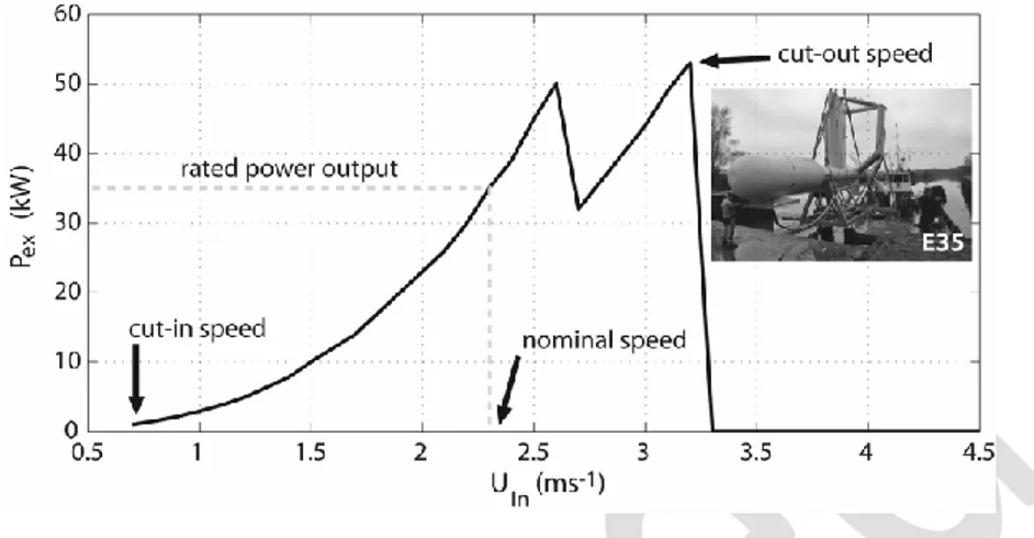
Figure 3. (A) Irish Sea numerical grid set-up with the prescribed model boundaries and 1-km resolution; 232
(B) a zoom-in to the area of interest, Sanda Sound, Kintyre Peninsula with a 250-m-resolution grid, with
233
the white box representing the area of interest for the deployment of an array of E35 devices.
234 235
To set up both models, rectilinear orthogonal grids in Cartesian coordinates were built
236
using Delft dashboard utilities and a compilation of available bathymetric data. It is
237
important to note that the chosen model resolutions are uniquely related to the available
238
bathymetry data and can therefore be further improved when high-resolution data are
239
available (for example, multi-beam bathymetry would provide a resolution of 2 m and
240
would allow a model to be nested at the turbine scale). The vertical resolution is
241
provided via sigma level coordinates to allow for a free surface. The datasets used for
242
modelling set-up are described in Table 2. The coarse-resolution study domain was
243
divided by 410 × 406 grid points in the 𝑀 and 𝑁 directions, respectively, resulting in
244
grid cell dimensions of 1 km × 1 km. At the model boundary (blue lines in Fig. 3A), the
245
sea level was prescribed using the ranges of the main tidal constituents by computing
246
the tidal elevation at the boundaries for each time step. The Delft dashboard has a ‘Tide
247
Stations’ toolbox (using both IHO and XTide stations) that allows the user to both view
248
and download water-level time series derived using astronomical constituents for a
249
selected tidal station and to directly define observation points in Delft3D-Flow.
250
The finer resolution was divided by 206 × 110 grid points in the 𝑀 and 𝑁 directions,
251
respectively, resulting in grid cell dimensions of 250 m × 250 m. At the open boundary
252
(green line in Fig. 3B), the water level was prescribed using the ranges of the
10
series values outputted from the coarse model run for each time step. Both models were
254
run on 3D mode with 3-sigma levels and the time step used was 15 s, which, according
255
to the Courant–Friedrichs–Levy criterion, is sufficiently small to ensure numerical
256
stability. The spatial discretisation of the horizontal advection terms was carried out
257
using the cyclic method, and time integration was based on the ADI method [18].
258 259
Table 2. Datasets used for the modelling set-up. 260
Type of Data Details Source
Bathymetry
2014. General Bathymetric Chart of the Oceans (GEBCO)
Coverage: Irish Sea
Resolution: 30 arc-second interval grid ~1 km
International Hydrographic Organization, Intergovernmental Oceanographic Commission, and
others
Bathymetry
2014. European Marine Observation and Data Network (EMODNet)
Coverage: Irish Sea Resolution: 250 m
EMODNet Bathymetry portal – http://www.emodnet-bathymetry.eu
National Oceanography Centre OceanWise Limited Bathymetry 2012. Multibeam H1355. Coverage: Kintyre Resolution: 2 m UK Hydrographic Office Currents
1993. Upward-looking, bottom-mounted ADCP Site (54°59.83N, 05°29.96W, water depth 139
m, Fig. 3). Part of a collection of sites used in the North Channel experiment (Challenger
Cruises)
Proudman Oceanographic Laboratory (now National Oceanography Centre)
Water levels 2015. Tidal gauge stations
International Hydrographic Organization, Intergovernmental Oceanographic Commission and
others
261
The water levels were computed at grid cell centres and velocity components were
262
defined at the midpoints of the grid cell faces (i.e., Arakawa-C staggered grids). The
263
horizontal large-eddy simulation (HLES) model for simulating horizontal turbulence
264
was combined with the use of the 𝑘 − 𝜀 turbulence model. HLES assumes that the
265
small-scale turbulent motions are isotropic, that is, they are not affected by large-scale
266
geometry. Because the objectives of the present work were to test the model sensitivity
267
in order to represent the far-wake modification related to tidal energy extraction, the
268
Delft3D-Flow module was run without wind and wind–wave forcing. The physical and
269
numerical parameters chosen for each model are provided in Table 3.
11
Table 3. Delf3D parameters for the hydro-morphodynamic transport model. 271
Parameters Model 1 Model 2
Resolution 1 km 250 m
Coordinate system Sigma Sigma
Grid points in M × N Directions 410 × 406 206 × 110
Number of layers 3 3
Time step 15 s 15 s
Forcing type Astronomical (IHO stations) Water-level time series generated from Model 1
Reflection parameter alpha (s2) 1000 1000
Water density (kgm−3) 1025 1025
Gravity (m2s−1) 9.81 9.81
Roughness (m1/2s−1, Chezy)* 100 100
Horizontal eddy viscosity (m2 s−1) 10 1
Horizontal eddy diffusivity (m2
s−1)
10 n/a
Vertical eddy viscosity (m2 s−1) n/a 1
Model for 2D turbulence Sub-grid scale HLES Sub-grid scale HLES
Model for 3D turbulence n/a k-Epsilon
* value determined using Eq. 5 for an average depth of 20 m (E35 deployment depth) and using the Manning–Strickler law (𝛼 =
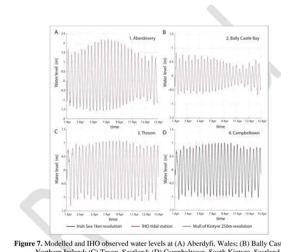
272
0.0474; 𝛽 = 1/3 [19]
273 274
The Irish Sea hydrodynamic model was validated against a moored Acoustic Doppler
275
Current Profiler (ADCP) south of Kintyre Peninsula (54°59.83N, 05°29.96W, water
276
depth 139 m) deployed by the Proudman Oceanographic Laboratory (now National
277
Oceanography Centre, Liverpool) under the POL North Channel Experiment
278
(Challenger Cruises C106 and C107). The ADCP (Fig. 3A) was deployed at a fixed
279
depth (139 m), and ENU velocity components were measured from the sensor over a
280
range of depths every 10 min (cell size= 8 m). The equipment return 78% of good data
281
collecting instantaneous velocities between 24-127 m due to the side lobe interference at
282
surface (no data between 0-24 m) and blanking (no data between 127-139 m). To
283
extrapolate the missing data at surface and bottom the 1/6 power law was applied. The
284
instantaneous measurements (i.e. real and extrapolated at 8 m intervals) were then
285
integrated through the water column to obtain depth-averaged velocity and direction
286
values to be compared with the model output.
287
Calibration tests were performed to match modelled and measured water levels using
288
the tidal observation stations inside each domain by altering grid properties (e.g.,
289
number of cells and grid refinement), boundary conditions (e.g., type and number of
290
boundaries and reflection parameter alpha), physical parameters (e.g., roughness and
291
horizontal eddy viscosity), and numerical parameters (e.g., smoothing time). Of all the
292
parameters analysed, the velocity field is most sensitive to the input model roughness.
293
As in hydraulic engineering, Delft3D uses a resistance coefficient (e.g., Chezy’s
12
Coefficient 𝐶 or Manning’s 𝑛) as input for bottom roughness. For example, when
295
Chezy’s or Manning’s laws are written in a form applicable to the sea, they are related
296
mathematically to the bed properties [19]:
297
𝐶 ≈ [𝛼(𝑧0𝑔 ℎ)𝛽
]0.5 =ℎ𝑔𝑛1/32 (5)
298
where: ℎ is the water depth; 𝑔 is the acceleration due to gravity; 𝛼 and 𝛽 are constants
299
[19]; and 𝑧0 is the bed roughness length, which in rough hydrodynamic flow is ~𝑑50/
300
12, with 𝑑50 being the grain-size diameter. From observations made by diving transects
301
performed when installing the seabed umbilical apparatus and power export
302
infrastructure to shore, the Sanda Sound bottom properties were found to include gravel,
303
sand, mud, and shells. These bottom characteristics are in accordance with the
304
information provided on Admiralty Chart No. 2126 (e.g., G.S.M.Sh). The mean values
305
of 𝑧0 for a bottom with these sediment types is ~0.3 mm [19], which corresponds to a
306
value of 𝐶 of 90–100 m0.5/s for deployment depths of 20–25 m (the E35 deployment
307
depth).
308 309
3.2. Modelling tidal energy arrays 310
It is not yet computationally feasible to construct a numerical model capable of
311
resolving the sub-turbine-scale turbulence (~0.01 m) that is generated as a turbine turns
312
and of incorporating the 20–500 km of the coastal ocean around the site needed to
313
model tidal patterns in the region [8]. In investigations of coastal hydrodynamics, the
314
grid resolution tends to be low compared with the gradients of the water level, of the
315
velocity, and of the bathymetry (i.e., the hydrostatic pressure assumption may locally be
316
invalid). The incorporation of turbines into coastal models concerns mainly how the
317
drag forces associated with power extraction are modelled [8, 20]. The presence of
318
obstacles in the flow may generate sudden transitions from flow contraction to flow
319
expansion. The forces due to obstacles in the flow that are not resolved (sub-grid) on the
320
horizontal grid need to be parameterized. The energy extraction (𝑃𝑒𝑥, Js−1) can be
321
simulated, in principle, by applying an extraction-related retarding force on the flow
322
(𝑈𝐼𝑛, ms−1) using an actuator disc, which can be considered as the effective swept area
323
of a device, perpendicular to the undisturbed fluid flow:
324
𝐹𝑋 = −𝑈𝑃𝑒𝑥
𝐼𝑛 (6)
13
where 𝐹𝑋 (N) is the retarding force on the fluid as it passes through the disc. This
326
equation does not include the influence of fluid blockage that the technology may also
327
apply to the fluid [21]. The value of 𝐹𝑋 (Eq. 6) is normally derived from the most
328
established model for axial force on bodies generating axial resistance (such as a rotor)
329
in oscillatory flow, namely, Morison’s (1950) equation [22]. The Morison equation is
330
the sum of two force components: a drag force (𝐹𝐷) proportional to the square of the
331
instantaneous flow velocity and an inertia force (𝐹𝐼) in phase with the local flow
332
acceleration:
333
𝐹𝑋(𝑡) = 𝐹𝐷+ 𝐹𝐼 =12𝜌𝑈𝑖𝑛(𝑡)|𝑈𝑖𝑛(𝑡)|𝐴𝑇𝐶𝐷+ 𝜌𝑢̇𝑖𝑛(𝑡)𝑉𝑇𝐶𝑀 (7)
334
where: 𝐴𝑇 is the swept area (𝜋𝐷2/4); 𝑉𝑇 is the volume of the circumscribing sphere
335
(assuming disc-like bodies such as a rotor) (𝜋𝐷3/6); 𝑈
𝑖𝑛 and 𝑢̇𝑖𝑛 are the flow velocity
336
and acceleration, respectively; 𝜌 is the fluid density; and 𝐶𝐷 and 𝐶𝑀 are two empirical
337
hydrodynamic coefficients, the drag and inertia coefficients, respectively, given by:
338 𝐶𝑀 = 6<𝐹𝑋𝑢̇𝑖𝑛> 𝜌𝜋𝐷3<𝑢̇𝑖𝑛𝑢̇𝑖𝑛> (8) 339 𝐶𝐷 = 𝜌𝜋𝐷28<𝐹<𝑈𝑋𝑈𝐼𝑛> 𝐼𝑛𝑈𝐼𝑛|𝑈𝐼𝑛|> (9) 340
In Delft3D-Flow, obstacles in the flow are denoted as hydraulic structures [17]. These
341
hydraulic structures should be located at velocity points of the staggered grid. To model
342
the force on the flow generated by a hydraulic structure, the flow in a computational
343
layer is blocked. Because a hydraulic structure generates a loss of energy besides that
344
caused by bottom friction, an additional force term is added to the momentum equation
345
to parameterize the extra loss of energy. With respect to Froude’s actuator disc theory, a
346
porous plate is used by Delft3D as the hydraulic structure for representing a turbine, that
347
is, a partially transparent structure that extends to the flow along one of the grid
348
directions. Details on modelling tidal energy extraction in coastal models using the
349
actuator disc theory are given by Draper et al. [23].
350
The principle differences between using porous plates and actual TECs are as follows:
351
(1) the momentum is extracted from the flow and not converted into mechanical motion
352
of the rotor; (2) vortices shed from the edge of the plate differ from those caused by the
353
blades of the TECs; and (3) the swirl angle of the flow from the porous plate is zero
354
[20]. These effects are exclusive to the far wake, and the modelling of TECs in Delft3D
355
focuses on the far-wake effects of the TECs [24]. Thus, it can be assumed that the far
14
wake is influenced only by the thrust, the diameter of the TECs, the ambient turbulence,
357
and, to a lesser extent, the turbine-generated turbulence.
358
When the turbine rotor extracts power from the fluid (Eq. 6) this manifests as a pressure
359
drop and a lower fluid velocity behind the rotor plane (Fig. 4A), which in turn manifests
360
as a thrust force, 𝐹𝑋. Owing to the pressure drop, momentum is extracted. The pressure
361
is assumed to be uniform over the area of the disc. The pressure drop is followed by a
362
decay of the velocity downstream of the disc. Consequently, the control volume
363
expands to satisfy the conservation of mass, that is, the loss of momentum induces a
364
wake. The wake can greatly influence the efficiency of a TEC positioned in the wake of
365
another TEC, for example, in tidal arrays.
366 367
368
Figure 4. (A) A turbine in a volume-constrained 2D flow field; (B) TEC domain represented as porous 369
plates to simulate flow blockage (adapted from [21]).
370 371
The porosity of the plate is controlled by a quadratic friction term to simulate the energy
372
losses and is used to add the momentum sink in the governing momentum equations
373
(Eq. 2), representing the pressure drop across the rotor and simulating the extraction of
374 energy (Fig. 4B): 375 𝜕𝑈 𝜕𝑡 + 𝑈 𝜕𝑈 𝜕𝑥 + 𝑉 𝜕𝑈 𝜕𝑦− 𝑓𝑉 = 𝜕 𝜕𝑥(𝜇 𝜕𝑈 𝜕𝑥) + 𝜕 𝜕𝑦(𝜇 𝜕𝑈 𝜕𝑦) − 1 𝜌( 𝜕𝑝 𝜕𝑥) + 𝑓𝑥− 𝑀𝜉 (10) 376
15
where: 𝜇 is the kinematic water viscosity; 𝑓𝑥 is the horizontal Reynolds stresses; and 𝑀𝜉
377
is the source or sink of momentum in the 𝜉 (or x) direction (i.e., perpendicular to the
378
flow), given by:
379
𝑀𝜉 = −𝐶𝑙𝑜𝑠𝑠𝑈𝐼𝑛 2
Δ𝑥 (11)
380
𝑀𝜉 has the form of an acceleration term (ms−2), where 𝐶𝑙𝑜𝑠𝑠 is the quadratic friction
381
coefficient and input term in the model, 𝑈𝐼𝑛 is the velocity in the 𝜉 (or x) direction, and
382
Δ𝑥 is the cell width in the x direction (held at the v-point of cell 𝑀, 𝑁). During the
383
simulation, it is assumed that the hydraulic structure is a “sub-grid” and that there is a
384
local equilibrium between the force and the flow due to the obstruction (i.e., generated
385
by the turbine) and the local water-level gradient.
386
The drag force (𝐹𝐷) in the direction of the fluid is the thrust (𝑇), namely, a mechanical
387
force generated by the contact of and interaction between a solid object and any fluid
388
(derived from Eq. 7). Conceptually, for a simple array of identical turbines, the total
389
drag force of N turbines (𝐶𝐷,𝑡𝑜𝑡𝑎𝑙) can be split into two parts, one due to
support-390
structure drag and another due to power extraction [8]:
391
𝐶𝐷,𝑡𝑜𝑡𝑎𝑙 =2𝐴𝑁
𝑐(𝐴𝑠𝐶𝑠+ 𝐴𝑇𝐶𝑇1) (12)
392
where: 𝑁 is the total number of turbines; 𝐶𝑇1 is one turbine’s thrust coefficient based on
393
the area swept by the blades 𝐴𝑇; 𝐶𝑠 is the gross drag coefficient of the structure
394
supporting one turbine, for example, the fairing and mooring lines, based on their
395
frontal area 𝐴𝑠; and Ac is the channel cross-sectional area. It is important to consider the
396
drag from the supporting structure of the turbine, because this drag can make a
397
significant contribution to the energy removed from the flow [8, 25]. Thus, the total
398
drag force on the fluid (𝐹𝐷,𝑡𝑜𝑡𝑎𝑙) due to power extraction by an array is typically
399
expressed as a quadratic drag law of the form:
400
𝐹𝐷,𝑡𝑜𝑡𝑎𝑙 = 𝜌𝐶𝐷,𝑡𝑜𝑡𝑎𝑙 𝐴𝑐𝑈𝑖𝑛2 = 𝜌𝑁2(𝐴𝑠𝐶𝑠+ 𝐴𝑇𝐶𝑇1)𝑈𝐼𝑛2 (13)
401
The momentum loss term (𝑀𝜉) can be written as a relationship between the total drag
402
force and the mass of one Delft3D grid cell:
403 −𝜌 𝑁 2(𝐴𝑠𝐶𝑠+𝐴𝑇𝐶𝑇1) 𝑈𝐼𝑛2 𝜌∆x∆yH = −𝐶𝑙𝑜𝑠𝑠 𝑈𝐼𝑛2 Δ𝑥 (14) 404
16
where H is the cell depth and ∆y is the cell size in the y direction (perpendicular to the
405
flow, in rectilinear grids ∆y = ∆x), which results in a relationship for determining 𝐶𝑙𝑜𝑠𝑠:
406
𝐶𝑙𝑜𝑠𝑠 =𝑁(𝐴𝑠𝐶𝑠+𝐴𝑇𝐶𝑇1)
2∆yH (15)
407
In channels with complex bathymetry, the free-stream flow may differ for each turbine.
408
For the purpose of simplification, here all the turbines are assumed to experience the
409
same free-stream flow and to have the same drag coefficient. Thus, the force on one
410
turbine and the power produced by one turbine in an array can be expressed as [8]:
411
𝐹1 = 𝜌2(𝐴𝑠𝐶𝑠+ 𝐴𝑇𝐶𝑇1)|𝑈𝐼𝑛|𝑈𝐼𝑛 (16)
412
𝑃1 =𝜌2(𝐶𝑃1𝐴𝑇)|𝑈𝐼𝑛|3 (17)
413
where 𝐶𝑇1 is the thrust coefficient of a single turbine and 𝐶𝑃1 is the power coefficient.
414
After determining the above values, the user can adjust the model by (1) manipulating
415
the aggregated drag coefficient of the array, 𝐶𝐷,𝑡𝑜𝑡𝑎𝑙 (Eq. 12), or (2) by manipulating the
416
individual drag coefficient of the turbine, 𝐶𝑇1. The value of 𝐶𝑇1 can be estimated using
417
the efficiency curve for a generic tidal turbine and the properties of prototypes (Fig. 5;
418
Table 1). The 𝑃𝑒𝑥 – 𝑈𝑖𝑛 E35 curve (Fig. 5) as well as values of 𝐶𝐷 were obtained from
419
OceanFlow Energy, and are based on scaling test values obtained from the wind–wave–
420
current tank at Newcastle University using a 1:40 scale model and tests performed at
421
Strangford Narrow using a 1:10 scale model. Both series of tests measured power
422
output, shaft speed, torque, and the drag experienced by the device under the influence
423
of variables such as inflow velocity, operating depth, wave period and amplitude,
424
pitch/yaw angles of the turbine, and blade pitch angle.
425
The E35 is linked to a control unit onshore. As waves build up in height the
426
instantaneous flow speed as a wave crest passes the rotor will exceed the rated flow
427
speed which is nominally 2.3 m/s. When the device sees around 2.5 ms-1 the generator
428
is at its maximum overload rated output (i.e. 52.5 kW) and is operating at or close to the
429
peak Cp value. When the control system detects that the flow is exceeding 2.5 ms-1 it
430
increases the load on the generator until the rotor is working at a lower tip speed ratio
431
and moves into the stall regime. The rotor is less efficient when working in the stall
432
regime so there is an immediate drop off in power output (see Fig. 5). If the waves
433
continue to get larger then as the peak velocity increases with wave height the
434
instantaneous power output continuous to rise. When the control system logs that the
17
rotor is already operating in the stall regime and that the power is consistently
436
exceeding the maximum instantaneous output of around 50 kW then it will shut down
437
the turbine by applying the brake and only allow the brake to be released when the
438
sampled peak flow speed consistently falls below 3.0 ms-1.
439 440
441
Figure 5. Power curve of the E35 Evopod for the 1:4 scale model deployed at Sanda Sound, South 442
Kintyre (Argyll, Scotland).
443 444
The total drag of the model was measured via load cells, and the thrust (from the rotor
445
spinning) was estimated by subtracting the other Evopod drag components (e.g.,
446
mooring lines, the presence of the supporting structure of the rotor itself) from the total
447
drag. The robustness of the physical tank results was confirmed by comparing them
448
with theoretical values computed using the blade element momentum (BEM) theory
449
[26, 27]. As the grid spacing is dependent on the bathymetric data available (i.e., 250 m
450
resolution), the “distributed-drag approach” [8] was used by enhancing the natural
451
bottom drag coefficient, 𝐶𝐷,𝑡𝑜𝑡𝑎𝑙, over the area spanned by the array. The model uses a
452
“sigma” coordinate system, which means that the thickness of the vertical layers
453
changes as the water level rises and falls according to tidal movements. The position of
454
a porous plate is specified in terms of these layers. Because the porous plates are
455
represented in grid cells of ~20–25 m depth, the first sigma layer is 33.3% of the total
456
depth (i.e., the first ~7 m of the water column). For a floating turbine with a rotor
457
diameter of 4.5 m, the extraction always occurs between the water line and a depth of
458
~7 m, independently of the rise and fall of the water column as the tide ebbs and floods.
459
Since an area of 50 m × 50 m is required for the moorings of each E35 device, each cell
460
can fit approximately five turbines, and 𝐶𝐷,𝑡𝑜𝑡𝑎𝑙 and 𝐶𝑙𝑜𝑠𝑠 were determined using
18
Equations 12 and 15, respectively (Table 4). The power available at each grid cell is
462
directly related to the inflow velocity to which the turbine is exposed. The rotor
463
diameters of TECs are dimensioned to approximately half the water depth, and, in
464
general, TECs convert 30% to 40% of the available energy in the current flowing
465
through the rotor into electrical power.
466 467
Table 4. Drag force (Fd) and array drag coefficient (CD,total) values based on the Evopod E35 𝑈𝐼𝑛–𝑃𝑒𝑥
468
curve and characteristics. Array drag coefficient values were determined considering a grid cell size of
469
250 m, five turbines per cell (all operating at nominal velocity), and a cell depth (H) of ~20 m.
470 471
Parameter Description Value
D Diameter of the rotor (m) 4.5
As TEC frontal area (m2) 20.3
AT Rotor swept area (m2) 16
Cs Gross drag coefficient of the structure 0.19
CT Thrust coefficient 0.71
L TEC length (m) 13
B TEC beam (m) 4.5
VT Volume of the circumscribing sphere (m3) 47.7
UIn Nominal speed (ms−1) 2.3
d Depth of the cell (m) 20
Fd Drag force at nominal speed (N) 30435
CD,total Array drag coefficient 0.012
472
For the particular case of the E35 device, the influence of the rotor occupies ~33% of
473
the water column. Assuming that the turbines are oriented cross-flow, the inflow
474
velocity is one-third of the cross-flow component at the depth outputted from the
475
Delft3D (i.e., the first sigma cell). Thus, five turbines each with a diameter of 4.5 m
476
occupying a grid cell of 250 m means that the total area occupied by E35 devices is
477
~10% of the grid cell size. The potential extractable kinetic power produced by a single
478
E35 device is given by:
479
𝑃𝐸35= 12𝜌𝐶𝑝𝐴𝑇𝑈𝐼𝑛3 (18)
480
where 𝐶𝑝 is the power coefficient, that is, the effectiveness of a turbine at a specific
481
flow velocity. For simplicity, and according to the flume tests, 𝐶𝑝~ 0.33 for the E35. A
482
depiction of the layout is given in Figure 6.
19
The device capacity factor is the ratio of the actual energy produced per annum divided
484
by the potential energy produced if the device was working continuously at its rated
485
output. The potential energy recovered over a year is given by:
486
𝐸𝐴𝑛𝑛𝑢𝑎𝑙 =12𝜌𝐶𝑝𝐴𝑇𝑈𝑚𝑎𝑥3 43𝜋𝑇 (19)
487
where 𝑇 is the annual period and 𝑈𝑚𝑎𝑥 is the nominal velocity. Therefore the energy
488
produced by a device in sinusoidal flow is only 3𝜋4 or 0.424 times that produced in a
489
steady current of the same maximum speed [28].
490 491
492
Figure 6. Sketch of the layout of the Evopod E35 turbines at Sanda Sound with power take-off (PTO) to 493
shore. Turbines are represented as porous plates at several grid cells of 250 m × 250 m in the Delft 3D
494
hydrodynamic model. The grid area represents a location inside the white box of Figure 3A. The grey grid
495
cells are blocked to simulate the extraction of energy by the momentum loss term (𝐶𝑙𝑜𝑠𝑠). Velocity deficit
496
and water-level differences are assessed in grid cells up current and down current of the porous plates
497
(i.e., cells ABC, DEF, and GHI).
498 499
The reference situation is the model run without turbines. The two analysed scenarios
500
are: (S1) the placement of a row of 15 turbines (Pplates 1–3) from N to S occupying
20
750 m of the channel area between cells ABC and cells DEF; and (S2) the placement of
502
two rows with a total of 30 turbines, 15 from N to S occupying 750 m of the channel
503
area between cells ABC and cells DEF, and the other 15 (Pplates 4–6) from N to S
504
occupying another 750 m of the channel area between cells DEF and cells GHI (Fig. 6).
505
One-month model runs were used to assess the energy production and hydrodynamic
506
impact of the tidal array by simulating both the momentum extraction and the induced
507
far-wake effect of each array scheme, comparing the velocity field with and without the
508
inclusion of porous plates for point locations (i.e., cells ABC, DEF, and GHI),
509
immediately upward and downward of the array scheme.
510
The velocity deficit (𝑈𝐷) is determined by:
511
𝑈𝐷 = (𝑈𝐼𝑛−𝑈𝑇
𝑈𝐼𝑛 ) (20)
512
where 𝑈𝑇 is the velocity at the cell with turbines represented as porous plates.
513
Differences in water elevation (𝑊𝐿𝐷) were determined for each cell (A–G, Fig. 6) by
514
subtracting the water elevation output from the no-extraction scenario. By including the
515
porous plates as an analogy to the disc theory, a pressure drop is formed close to the
516
porous plate. This pressure drop manifests as a thrust force (𝐹𝐷,𝑡𝑜𝑡𝑎𝑙), and momentum is
517
extracted (𝑀𝜉). The pressure is assumed to be uniform over the area of the porous plate.
518
The pressure drop is followed by a decay of the velocity downstream of the disc (𝑈𝐷).
519
Consequently, the control volume expands to satisfy the conservation of mass. The
520
𝐶𝐷,𝑡𝑜𝑡𝑎𝑙 is dependent on the operational conditions, which means that 𝐶𝑙𝑜𝑠𝑠 should be
521
modified by considering the inflow velocity at the entry of the rotor. This is not yet
522
possible using coastal models such as Delft3D, and therefore simulations must be
523
performed using a constant coefficient.
524 525 4. Results 526 4.1.Model Validation 527
A comparison between measured and modelled water levels was performed for four
528
sites located in the Irish Sea covering the spring and neap periods (Fig. 7). For site 1
529
(Aberdyfi, circle 1 in Fig. 3A), located on the eastern coast of Ireland and close to the
530
model boundary, the agreement is good (r2 = 0.96, RMSE = 0.20 m). The model
531
performs slight better during high tide, under predicting the peak water levels at low
21
tide, especially during spring tides (Fig. 7A). For sites 2 (Bally Castle Bay, Northern
533
Ireland) and 3 (Troon, west coast of Scotland) (circles 2 and 3 in Fig. 3A, respectively),
534
which are closer than site 1 to the Kintyre Peninsula, the agreement is very good (r2 =
535
0.99, RMSE = 0.01 m) during the spring–neap cycle (Fig. 7B–C). Finally, for site 4
536
(Campbeltown, located north of Sanda Sound on the Kintyre Peninsula) (circle 4 in
537
Fig. 3), the agreement between modelled values and the IHO tidal station values is
538
overall very good (r2 = 0.99, RMSE = 0.01 m), particularly considering that site 4
539
belongs to both the coarse- and medium-resolution models.
540 541
542
Figure 7. Modelled and IHO observed water levels at (A) Aberdyfi, Wales; (B) Bally Castle Bay, 543
Northern Ireland; (C) Troon, Scotland; (D) Campbeltown, South Kintyre, Scotland.
544 545
A comparison between measured and modelled depth-averaged current speeds and
546
current directions was performed for the POL ADCP site (see location in Fig. 3). In
547
general, the agreement is very good: r2 = 0.83, RMSE = 0.09 ms−1 for the current speed;
548
and r2 = 0.84, RMSE = 30° for the current direction (Fig. 8). Overall, the
coarse-549
resolution model is able to reproduce the water level, current speed, and current
550
direction observed at the IHO tidal stations and those obtained using ADCP
22
measurements. The coarse-resolution model can therefore be used with confidence to
552
generate the boundary conditions for the medium-resolution model.
553 554
555
Figure 8. Modelled and measured (A) current speed and (B) current direction at a point south of Kintyre 556
Peninsula in the Irish Sea (54°59.83N, 05°29.96W, water depth 139 m).
557 558
4.2. Energy extraction simulations 559
The modelled cross-rotor flow for the top third of the water column during the peak ebb
560
of spring tides is shown in Figure 9A, and the cross-rotor flow velocity magnitude and
561
potential extractable power for a single E35 device are displayed in Figure 9B and C,
562
respectively. Assuming a constant 𝐶𝑝 in Equation 18, and taking into account the porous
563
plate locations (see Fig. 6), the potential extractable power of five turbines for a grid
564
cell was modelled and is shown in Figure 10. Each plot in Figure 10 shows the annual
565
power output in MWh, obtained by integrating the hourly results of extractable kinetic
566
power throughout the analysed month and then multiplying by 12 months. For a total of
567
30 E35 turbines (with a total installed capacity of ~1 MW), the total power output is
568
~1500 MWh (five E35 devices per cell), with values ranging between 168 and
569
303 MWh. The range in power output values clearly reflects the importance of choosing
570
the location of the array, as slight changes in the location (of <1 km) can approximately
571
double the potential power output.
572 573
23 574
Figure 9. (A) Modelled cross-rotor flow for the top third of the water column during peak ebb of spring 575
tides, showing the area of interest around the location of the currently deployed E35 device (white box);
576
(B) representative flow velocities for a grid cell inside the area of interest (𝑈𝐼𝑛); (C) potential extractable
577
power for a single E35 device for a representative month. The black box marks the maximum potential
578
kinetic power extracted by a single device at peak flow (spring tides, ~30kW).
579 580
581
Figure 10. (A–F) Extractable power (kW/cell) and annual power output estimates (MWh) for each grid 582
node location represented by a 250 m × 250 m cell size in which five E35 devices are hypothetically
583
placed, extracting power in the top third of the water column (~20 m depth), and assuming a constant
584
power coefficient (𝐶𝑝) and uniform flow (𝑈𝐼𝑛).
585 586
The effect of the turbines was then included as a loss in the momentum equations
587
according to the above scenarios (as represented in Fig. 6) and by choosing an area
588
within the model where cell depths were ~20–25 m. The results for velocity deficit (𝑈𝐷)
589
and water-level differences (𝑊𝐿𝐷) for scenarios S1 and S2 are shown in Figs. 11 and
590
12, respectively. For S1, and for one-month simulations, the mean values of 𝑈𝐷 varied
591
from ~0.035 ms−1 (Cells A and D), to ~0.02 ms−1 (Cells B and E), and to ~0.03 ms−1
24
(Cells C and F). Maximum flow alterations ranging from 0.07 up to 0.16 ms−1 were
593
registered. For water-level differences, the mean 𝑊𝐿𝐷 ranged between 1.6 and 2.0 mm
594
with maximums of ~8.5–11.0 mm.
595 596
597
Figure 11. (A–F) Estimated velocity deficit (𝑈𝐷, A1–F1) and water-level differences (𝑊𝐿𝐷, A2–F2)
598
determined for the cells upward (ABC) and downward (DEF) of porous plates 1 to 3. The momentum loss
599
was determined with a constant 𝐶𝑙𝑜𝑠𝑠 assuming that the E35 devices were working at nominal velocity.
600 601
Adding more turbines to the model directly increases the values of both 𝑈𝐷 and 𝑊𝐿𝐷
602
(Fig. 12). S2 was run with six porous plates representing the energy extraction of 30
603
turbines (i.e. installed capacity 1050kW) hypothetically placed with an interval of three
604
cells between two groups of 15 turbines (i.e., 15 turbines upward and 15 downward of
605
cells DEF, Fig. 6). The mean 𝑈𝐷 is ~0.1 ms−1 for cells A, D, and G, ~0.07 ms−1 for cells
25
B, E, and H, and ~0.08 ms−1 for cells C, F, and I. However, the maximum flow
607
alterations have a greater influence on velocity deficit, with values of 0.30, 0.35, and
608
0.30 ms−1 (cells A, D, and G, respectively), 0.25, 0.42, and 0.38 ms−1 (cells B, E, and H,
609
respectively), and 0.2, 0.4, and 0.5 ms−1 (cells C, F, and G, respectively). With respect
610
to water-level differences, the mean 𝑊𝐿𝐷 ranges between 2.1 and 5.1 mm with
611
maximums of ~13–26 mm. These results show that doubling the installed capacity has
612
the effect of approximately doubling the mean velocity deficit and water-level
613
differences and of increasing by a factor of 4 the registered maximum values of 𝑈𝐷 and
614
𝑊𝐿𝐷, mainly during spring tides.
615 616
617
Figure 12. (A–I) Estimated velocity deficit (𝑈𝐷, A1–I1) and water-level differences (𝑊𝐿𝐷, A2–I2)
618
determined for the cells upward (ABC), central (DEF), and downward (GHI) with respect to porous plates
619
1 to 6. The momentum loss was determined with a constant 𝐶𝑙𝑜𝑠𝑠 assuming that the E35 devices were
620
working at nominal velocity.
621 622
26 4.3.Capacity Factor of a small array 623
Based on the modelling simulations annual power output estimates (MWh) for each grid
624
node location were determined (Fig. 11) considering the placement of five E35 devices
625
for node on a total of 30 turbines. Considering the nominal velocity on Eq.19 and if a
626
tidal variation is assumed to be sinusoidal then the theoretical capacity factor is the area
627
under the sinusoid is 0.424 times the peak output (power output at peak flow speed).
628
Likewise, if a neap tide is half the speed of a spring tide then the theoretical capacity
629
factor over a lunar month drops to 0.212 times the peak output. Other capacity factors
630
can be determined e.g. if the 2nd tide is only 80% of the first tide, which is not
631
uncommon, then the theoretical capacity factor drops further to 0.17. However by rating
632
the turbine to give its peak output at less than the maximum spring tide flow speed it is
633
possible to push up the capacity factor and a value of 0.30 is reasonable. Based on the
634
results obtained by the model simulations, Table 5 presents the capacity factors
635
calculated for each of the grid nodes.
636 637
Table 5. Summary of the capacity factors and total annual output (MWh) based on the simulations 638
performed for a small array of floatable E35 devices placed at Sanda Sound.
639
Parameter Pplate1 Pplate2 Pplate3 Pplate4 Pplate5 Pplate6
Rated output (kW) 35 35 35 35 35 35
Annual power output per turbine (MWh)
40.2 56.2 57.8 33.6 47 60.6
Capacity Factor 0.14 0.20 0.21 0.12 0.17 0.22
Number of turbines 5 5 5 5 5 5
Total Installed Capacity (all turbines) (kW)
175 175 175 175 175 175
Total Annual Output (all turbines) (MWh)
201 281 289 168 235 303
640
Considering the rated output of E35 (35kW) and a capacity factor of 0.3, and assuming
641
fix other parameters such as 𝐶𝑝 (0.33), transmission efficiency (96%) and availability
642
(95%), the theoretical annual output for a single turbine is 84 MWh which traduces to a
643
total of 2517 MWh for a small array of 30 E35 turbines (1050kW of installed capacity).
644
Based on the simulations performed within this paper (Fig. 11) the total annual output is
645
of 1477 MWh (Table 5) i.e. 59% of the theoretical annual output. The location
646
represented by Pplate6 reports the higher capacity factor, which means that if similar
647
locations were found a total of 1818 MWh of annual energy could be produced by a
648
small array of 30 turbines i.e. 72% of the theoretical annual output, representing an
649
increment of 13% on energy production in respect to the sketch alignment of Fig. 6.
27 5. Discussion
651
Hydrodynamic coastal models can be used to incorporate large numbers of turbines
652
using a coarse representation of the devices, such as presented in this paper. These
653
models are required for analysing fluid flows, improving complex simulation scenarios
654
prior to installing TECs, and establishing energy extraction maximum limits without
655
causing significant disturbances to the flow, to the sediment transport patterns, and to
656
channel cross-section stability [7–8, 20, 29–30]. Currently, little is known about the
657
environmental effects of TEC devices. To successfully perform environmental impact
658
studies with respect to such devices, it is essential to understand the local
659
hydrodynamics, namely, how flow varies naturally and how any proposed tidal energy
660
array compares with such natural variability [30-32].
661
The tidal energy industry is reaching commercial status following the testing of
662
different TEC prototypes in recent years. The next logical step for the industry is the
663
installation of multiple devices in arrays. The “distributed-drag approach” used in the
664
present study is able to give a good indication of the potential power that can be
665
extracted by these device arrays. Results from the simulations performed here showed
666
that for the selected location, a 1-MW installed capacity at Sanda Sound Channel with
667
E35 Evopod floatable devices can yield a combined annual power output of
668
~1500 MWh. Using porous plates in locations with high resource potential, and
669
assuming that equivalent locations could be found within or in the vicinity of Sanda
670
Sound, the annual maximum power output for the same installed capacity could reach
671
>2500 MWh (considering a capacity factor of 0.3).
672
The values for power output calculated in the present study are slightly lower than those
673
obtained from preliminary spectral modelling provided by consultants Aquamarine
674
Power, who calculated a total annual power output of 2500–3100 MWh for a 1-MW
675
tidal array deployed at Sanda Sound [13]. However, as demonstrated in the present
676
study, slight alterations in inflow velocities caused by differences in device location of
677
just 1 km can double the power output. These results are important since show that
678
small alteration on the flow related to the placement of turbines can change
679
considerably the annual power output. Therefore, resource assessments of power output
680
for a given site using coastal models provide a good preliminary evaluation that should
681
be complemented with detailed ADCP measurements. The use of floatable and smaller
682
devices such as the E35 has obvious advantages, because these devices can be easily