Revista Brasileira de
Engenharia Agrícola e Ambiental
Campina Grande, PB, UAEA/UFCG – http://www.agriambi.com.br
v.20, n.6, p.551-556, 2016
Non-destructive models for leaf area determination in canola
Francilene de L. Tartaglia
1, Evandro Z. Righi
1, Leidiana da Rocha
1,
Luis H. Loose
2, Ivan C. Maldaner
3& Arno B. Heldwein
1 DOI: http://dx.doi.org/10.1590/1807-1929/agriambi.v20n6p551-556A B S T R A C T
The leaf is a very important structure of the plants, since it allows gas exchanges and the transformation of light energy into chemical energy. This study aimed to generate and test mathematical models for leaf area estimation in canola based on leaf dimensions. Two experiments were conducted with canola in 2014, in which leaves were collected in different phenological stages with different sizes and shapes. Subsequently, leaf length, width and area were measured (with automatic meter) in 606 leaves, which included 371 ovate and 235 lanceolate leaves. The models were generated using length, width and length versus width as independent variables and leaf area as dependent variable. The models were validated using a group of leaves different from those used to generate the models. A total of 27 models were obtained and those with best statistics and higher simplicity were selected. The polynomial model LA = 0.88735 W2 + 0.93503 W and the power model LA = 1.1282 W1.9396 can be
used for both types of leaves and have high accuracy in the estimation of canola leaf area.
Modelos não destrutivos para determinação
da área foliar em canola
R E S U M O
A folha é uma estrutura de grande importância para as plantas, visto que por meio dela ocorrem as trocas gasosas e a transformação da energia luminosa em energia química. O objetivo neste trabalho foi gerar e testar modelos matemáticos para a estimativa de área foliar de folhas de canola em função das dimensões foliares. Para isto foram realizados dois experimentos com canola no ano de 2014 e coletadas folhas em diferentes estágios fenológicos e de diferentes tamanhos e formas; posteriormente foram medidos o comprimento, a largura e a área foliar (com medidor automático) de 606 folhas dentre as quais 371 ovaladas e 235 lanceoladas. Os modelos foram gerados utilizando-se comprimento, largura e comprimento versus largura como variáveis independentes e a área foliar como variável dependente. Os modelos foram validados com um grupo distinto de folhas dos utilizados para a geração. Obteve-se o total de 27 modelos escolhendo-se aqueles que apresentaram as melhores estatísticas e maior simplicidade. Os modelos que podem ser utilizados para ambos os tipos de folhas e apresentam alta precisão de estimativa de área foliar em canola, são o modelo polinomial AF = 0,88735 L2 + 0,93503 L e o modelo potencial
AF = 1,1282 L1,9396.
Key words:
Brassica napus
ovate leaves lanceolate leaves modeling
Palavras-chave:
Brassica napus
folhas ovaladas folhas lanceoladas modelagem
1 Universidade Federal de Santa Maria/Centro de Ciências Rurais/Departamento de Fitotecnia. Santa Maria, RS. E-mail: [email protected]
(Corresponding author); [email protected]; [email protected]; [email protected]
2 Instituto Federal Forroupilha. Santo Ângelo, RS. E-mail: [email protected]
3 Instituto Federal Farroupilha. São Vicente do Sul, RS. E-mail: [email protected]
Introduction
Canola (Brassica napus L. var. oleifera) is a cold-season oilseed plant cultivated in Southern Brazil (Krüger, 2011). Its yield is influenced by different environmental, physiological and morphological factors, among which leaf area (LA) is a parameter indicative of crop yield, since biomass accumulation occurs through photosynthesis and the leaf is the main plant organ, responsible for gas exchanges and light energy interception (Pereira et al., 1997; Favarin et al., 2002).
Accurate LA measurements are essential to understand the interaction between plant growth and the environment in which they develop (Jesus et al., 2001). There are non-destructive methods for LA determination using simple and easily operated devices that preserve leaf integrity (Adami et al., 2008; Fagundes et al., 2009; Bakhshandeh et al., 2011). Some examples are models generated for tomato and cucumber (Blanco & Folegatti, 2003), melon (Lopes et al., 2007), sunflower (Maldaner et al., 2009) and crambe (Toebe et al., 2010).
For the canola crop, there are the models of Chavarria et al. (2011) and Cargnelutti Filho et al. (2015). However, applying only one model to determine canola leaf area may not be adequate, because the leaves are morphologically different along its development (Iriarte & Valetti, 2008) and one model for each cultivar becomes unviable, since new cultivars are frequently released. On the other hand, it is necessary to verify which is the variability existing between cultivars and cultivation environments for canola leaf area in the producing regions of Brazil. Thus, this study aimed to generate and test mathematical models for leaf area estimation in canola based on leaf dimensions.
Material and Methods
The experiment was carried out at the Department of Plant Science of the Federal University of Santa Maria (UFSM), in the municipality of Santa Maria, RS, Brazil (29° 43’ 23” S; 53º 43’ 15” W; 95 m). The climate of the region, according to Köppen’s classification, is Cfa, humid subtropical with hot summers and without a defined dry season (Heldwein et al., 2009). The soil in the experimental area is classified as sandy dystrophic Red Argisol (Streck et al., 2008). Soil correction and fertilization were based on its chemical analysis, following the recommendations of the manual of fertilization and liming for the states of Rio Grande do Sul and Santa Catarina (SBCS, 2004).
The spacing used in the first experiment was 0.30 m between rows and 0.08 m between plants, totaling a population of 416,666 plants ha-1;the second experiment used a spacing
of 0.50 m between rows and 0.06 m between plants, totaling a population of 400,000 plants ha-1. The first experiment was
sown on May 15, 2014, and emergence occurred on May 20, 2014; the second experiment was sown on June 9, 2014, and emergence occurred on June 15, 2014. The experiments were set in randomized blocks, in a split-plot scheme, with four replicates. Three manual weedings were performed for weed control, while pests (Diabrotica speciosa L.) were controlled through the application of insecticide in the vegetative stage.
Four canola cultivars were sown: Hyola 433, Hyola 411, Hyola 420 and Hyola 61. Three leaf collections were performed in these experiments, on July 28, July 29 and August 13, 2014, which encompassed the stages of formation of rosette, flower bud and flowering. Samples were collected in different phenological stages and in leaves of different sizes and shapes, because canola plants produce leaves of different shapes along the cycle.
These leaves with different shapes can be grouped into two distinct categories; the first one is called ovate and includes basal and petiolate leaves, arranged in the form of a rosette, while the second one, the lanceolate, refers to smaller leaves and amplexicaul leaves that emerge after stem elongation.
After plant collection, the leaves were separated from the stem and only those photosynthetically active, with no damage or deformation caused by diseases, insects or other external factors, were selected. Length, width and area were measured in these leaves, in a total of 606 leaves, 371 ovate and 235 lanceolate, with width from 0.3 to 16.5 cm, length from 1.8 to 22.5 cm and leaf area from 0.36 to 273. 97 cm².
Length (L) was measured with a graduated ruler, considering the length of leaf blade along the midrib, disregarding the petiole. Width (W) was determined by measuring the longest width of the leaves perpendicularly to the midrib. Leaf area (LA) for both types of leaves was obtained with a leaf area integrator (LICOR 3000).
The models were generated using length (L), width (W) and the product of length versus width (L.W) as independent variables, and the measured LA as dependent variable. Linear, quadratic, exponential and power models were obtained using the program Sigma Plot®. Models with distinction between ovate and lanceolate leaves were generated using 186 ovate leaves and 117 lanceolate leaves, while models without such distinction were generated using 303 mixed leaves. The aim was to identify which independent variable is best correlated with LA and whether a general model can be used to determine canola LA or if it is necessary to use one model for each type of leaf. The slope was estimated by forcing the line to pass through the origin (null intercept), because it is more correct according to Richter et al. (2014), since if there are no linear dimensions, there is no leaf area.
For validation, the obtained models were tested with a set of leaves different from those used to generate the models, but with the same number of mixed, ovate and lanceolate leaves. LA estimated by the mathematical model was compared with the LA measured through the analysis of data dispersion around the 1:1 line, in order to select the model in which the line generated between the values observed and obtained by the model was as close as possible to the 1:1 line.
model developed by Chavarria et al. (2011) in Passo Fundo, RS, was also tested, in order to verify whether this model was valid for both types of canola leaves.
Results and Discussion
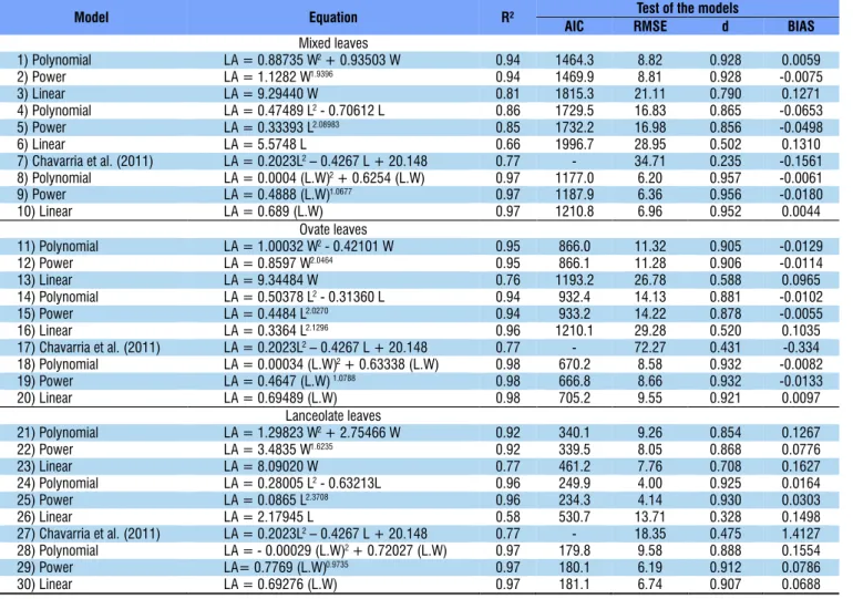
Initially, the relationship of length, width and length versus width (L.W) with leaf area was tested through linear, quadratic, power and exponential regressions. However, the exponential equations did not fit and were disregarded from the study. After this previous analysis, 27 linear, quadratic and power models were obtained (Table 1). Isolated models for each cultivar were also generated, but the coefficients of each model were similar to those of general models. Thus, there was no need for one model for each cultivar, which is desired, because new cultivars are released every year and it can disqualify the model for future use.
Canola leaf area is estimated with greater accuracy by the models that use the product of leaf Length x Width (L.W) as independent variable, compared with models that use only one leaf dimension (Table 1). Similar results were obtained by Hinnah et al. (2014), Serdar & Demirsoy (2006) and Keramatlou et al. (2015) for eggplant, chestnut and Persian walnut, respectively. This result occurs because the product
L.W is an area, thus requiring the adjustment of the reducing coefficients in each model.
For mixed leaves, LA is best estimated by polynomial and power equations, Models 8 and 9, respectively, which use L.W as independent variable. However, the Models 1 and 2, which use only width (W) as independent variable, show similar results, with the advantage of using only one variable, thus surpassing the models for ovate leaves when only W is used (Table 1).
LA is best estimated by the power equation, Model 19, for ovate leaves and by the power equation, Model 29, for lanceolate leaves. Both use L.W as independent variable (Table 1). When the choice is only one of the leaf dimensions to estimate leaf area, the independent variable with highest correlation with LA varies depending on the type of leaf. For lanceolate leaves, length (L) is the best variable to estimate LA, while width (W) is the best variable for ovate leaves. Thus, the power equations Model 12 for ovate leaves, which requires only the variable W, and Model 25 for lanceolate leaves, which requires only the variable L, show good results, with the advantage of using only one of the leaf dimensions.
The analysis of data dispersion around the 1:1 line indicates that some of the developed models show high capacity and accuracy for the estimation of canola leaf area (Figure 1).
Initially, due to the morphological difference between the leaves, the use of different models to accurately estimate canola
Model Equation R² Test of the models
AIC RMSE d BIAS
Mixed leaves
1) Polynomial LA = 0.88735 W2+ 0.93503 W 0.94 1464.3 8.82 0.928 0.0059
2) Power LA = 1.1282 W1.9396 0.94 1469.9 8.81 0.928 -0.0075
3) Linear LA = 9.29440 W 0.81 1815.3 21.11 0.790 0.1271
4) Polynomial LA = 0.47489 L2- 0.70612 L 0.86 1729.5 16.83 0.865 -0.0653
5) Power LA = 0.33393 L2.08983 0.85 1732.2 16.98 0.856 -0.0498
6) Linear LA = 5.5748 L 0.66 1996.7 28.95 0.502 0.1310
7) Chavarria et al. (2011) LA = 0.2023L2– 0.4267 L + 20.148 0.77 - 34.71 0.235 -0.1561 8) Polynomial LA = 0.0004 (L.W)2+ 0.6254 (L.W) 0.97 1177.0 6.20 0.957 -0.0061
9) Power LA = 0.4888 (L.W)1.0677 0.97 1187.9 6.36 0.956 -0.0180
10) Linear LA = 0.689 (L.W) 0.97 1210.8 6.96 0.952 0.0044
Ovate leaves
11) Polynomial LA = 1.00032 W2- 0.42101 W 0.95 866.0 11.32 0.905 -0.0129
12) Power LA = 0.8597 W2.0464 0.95 866.1 11.28 0.906 -0.0114
13) Linear LA = 9.34484 W 0.76 1193.2 26.78 0.588 0.0965
14) Polynomial LA = 0.50378 L2- 0.31360 L 0.94 932.4 14.13 0.881 -0.0102
15) Power LA = 0.4484 L2.0270 0.94 933.2 14.22 0.878 -0.0055
16) Linear LA = 0.3364 L2.1296 0.96 1210.1 29.28 0.520 0.1035
17) Chavarria et al. (2011) LA = 0.2023L2– 0.4267 L + 20.148 0.77 - 72.27 0.431 -0.334 18) Polynomial LA = 0.00034 (L.W)2+ 0.63338 (L.W) 0.98 670.2 8.58 0.932 -0.0082
19) Power LA = 0.4647 (L.W)1.0788 0.98 666.8 8.66 0.932 -0.0133
20) Linear LA = 0.69489 (L.W) 0.98 705.2 9.55 0.921 0.0097
Lanceolate leaves
21) Polynomial LA = 1.29823 W2+ 2.75466 W 0.92 340.1 9.26 0.854 0.1267
22) Power LA = 3.4835 W1.6235 0.92 339.5 8.05 0.868 0.0776
23) Linear LA = 8.09020 W 0.77 461.2 7.76 0.708 0.1627
24) Polynomial LA = 0.28005 L2- 0.63213L 0.96 249.9 4.00 0.925 0.0164
25) Power LA = 0.0865 L2.3708 0.96 234.3 4.14 0.930 0.0303
26) Linear LA = 2.17945 L 0.58 530.7 13.71 0.328 0.1498
27) Chavarria et al. (2011) LA = 0.2023L2– 0.4267 L + 20.148 0.77 - 18.35 0.475 1.4127 28) Polynomial LA = - 0.00029 (L.W)2+ 0.72027 (L.W) 0.97 179.8 9.58 0.888 0.1554
29) Power LA= 0.7769 (L.W)0.9735 0.97 180.1 6.19 0.912 0.0786
30) Linear LA = 0.69276 (L.W) 0.97 181.1 6.74 0.907 0.0688
The transverse line in each figure is the 1:1 line
Figure 1. Observed leaf area versus leaf area estimated using width (W), length (L) and length versus width (L.W) of canola leaves through various developed equations and the equation of Chavarria et al. (2011)
A. B.
C. D.
E. F.
G. H.
leaf area was expected to be necessary. However, according to the tests of the models, it is clearly possible to use one general model (with no difference regarding the type of leaf), since the RMSE of the model that uses L.W or only width (W) is lower than 8.82 cm², below the values obtained by Kumar (2009), Toebe et al. (2012) and Hinnah et al. (2014), who found minimum RMSE in their models of 71.79 for saffron, 12.56 for
The models selected to estimate leaf area in lanceolate and ovate leaves showed good results, with low RMSE, which varied from 4.14 to 11.28 cm² (Figure 1A; 1B; 1C and 1D), although the models proposed for lanceolate leaves slightly underestimated leaf area. Although these models have high accuracy, their use is more time-consuming, because it is necessary to collect data of leaf length and width, besides classifying leaves as ovate and lanceolate.
Therefore, the general model that uses L.W as independent variable, proposed for all types of leaves, showed excellent results, with data well distributed around the 1:1 line and RMSE of only 6.20 cm² (Figure 1E). Polynomial and power models, both using only width (W) as independent variable, showed high capacity to estimate canola leaf area, with data well distributed around the 1:1 line and RMSE of only 8.81 and 8.82 cm², respectively (Figure 1F and 1G), and with the advantage of using only one of the leaf dimensions, which reduces by 50% the number of measurements, decreasing the working time at the field. The measurement of only one variable is preferable, because, according to Kumar (2009) and Floriano et al. (2006), one must opt for the simplicity and convenience of the models used, provided that they show good fits to the data. These selected models also have lower AIC, d close to 1, and BIAS, close to zero.
The model proposed by Chavarria et al. (2011) was not able to estimate canola leaf area accurately, because it initially underestimates and then overestimates the values, without following the 1:1 distribution (Figure 1H). Its application resulted in the highest RMSE among the tested models (34.7, 72.27 and 18.35 cm²), which may have occurred because the authors did not force the equation to pass through the origin (null intercept), because the model estimates a leaf area of 20.148 cm² even when the independent variable (length) is equal to zero. According to Richter et al. (2014), it is important to force the linear regression to pass through the origin (null intercept), because if there are no linear dimensions, there must not be leaf area. Additionally, Chavarria et al. (2011) also used leaf length (L) as independent variable. However, the variable with highest correlation with canola leaf area when a general model is used is leaf width (W), which is corroborated by the results of Cargnelutti Filho et al. (2015).
The coefficients of the models obtained in the present study for four different cultivars were close to those obtained by Cargnelutti Filho et al. (2015) individually for three cultivars, indicating that one single model can be used for the different canola cultivars under the climatic conditions of Santa Maria-RS. In tests conducted with the equations of Cargnelutti Filho et al. (2015) for Hyola 61 and Hyola 433, with the equations specific for the LA of these cultivars, there was underestimation of more than 10% in the estimated values of LA compared with those in the present study. On the other hand, the general power equation (Model 2) showed deviations in the 1:1 tendency of at most 4% when the cultivars were separated, which demonstrate the capacity for LA estimation of mixed leaves of the power model developed in the present study.
Conclusions
1. Canola leaf area can be accurately estimated based on linear dimensions in a non-destructive way.
2. The morphological difference of the leaves does not have high influence on leaf area estimation, provided that the model based on length versus width (L.W) or only width (W) is used.
3. The polynomial model LA = 0.88735 W² + 0.93503 W and the power model LA = 1.1282 W1.9396 can be used for both
types of leaves and have high accuracy in the estimation of canola leaf area.
Literature Cited
Adami, M.; Hastenreiter, F. A.; Flumignan, D. L.; Faria, R.T. Estimativa de área de folíolos de soja usando imagens digitais e dimensões foliares. Bragantia, v.67, p.1053-1058, 2008. http://dx.doi. org/10.1590/S0006-87052008000400030
Bakhshandeh, E.; Kamkar, B.; Tsialtas, J. T. Application of linear models for estimation of leaf area in soybean [Glycine max (L.) Merr]. Photosynthetica, v.49, p.405-416, 2011. http://dx.doi. org/10.1007/s11099-011-0048-5
Blanco, F. F.; Folegatti, M. V. A new method for estimating the leaf area index of cucumber and tomato plants. Horticultura Brasileira, v.21, p.666-669, 2003. http://dx.doi.org/10.1590/S0102-05362003000400019
Cargnelutti Filho, A.; Toebe, M.; Alves, B. M.; Burin, C.; Kleinpaul, J. A. Estimação da área foliar de canola por dimensões foliares. Bragantia, v.74, p.139-148, 2015. http://dx.doi.org/10.1590/1678-4499.0388
Chavarria, G.; Tomm, G. O.; Muller, A. Mendonça, H. F.; Mello, N.; Betto, M. S. Índice de área foliar em canola cultivada sob variações de espaçamento e de densidade de semeadura. Ciência Rural, v.41, p.2084-2089, 2011. http://dx.doi.org/10.1590/S0103-84782011001200008
Fagundes, J. D.; Streck, N. A.; Kruse, N. D. Estimativa da área foliar de Aspilia montevidensis (Spreng.) Kuntze utilizando dimensões lineares. Revista Ceres, v.56, p.266-273, 2009.
Favarin, J. L.; Dourado Neto, D.; García, A. G. Y; Nova, N. A. V.; Favarin, M. Da G. G. V. Equações para a estimativa do índice de área foliar do cafeeiro. Pesquisa Agropecuária Brasileira, v.37, p.769-773, 2002. http://dx.doi.org/10.1590/S0100-204X2002000600005
Floriano, E. P.; Müller, I.; Finger, C. A. G.; Schneider, P. R. Ajuste e seleção de modelos tradicionais para série temporal de dados de altura de árvores. Ciência Florestal, v.16, p.177-199, 2006. Heldwein, A. B.; Buriol, G. A.; Streck, N. A. O clima de Santa Maria.
Ciência & Ambiente, v.38, p.43-58, 2009.
Hinnah, D. H.; Heldwein, A. B.; Maldaner, I. C.; Loose, L. H.; Lucas, D. D. P.; Bortoluzzi, M. P. Estimativa da área foliar da berinjela em função das dimensões foliares. Bragantia, v.73, p.213-218, 2014. http://dx.doi.org/10.1590/1678-4499.0083
Iriarte, L. B.; Valetti, O. E. Cultivo de colza. – 1.ed. – C. A. de Buenos Aires: Instituto Nacional de Tecnologia Agropecuária, 2008. 156p. Jesus, W. C. de; Vale, F. X. R. do; Coelho, R. R.; Costa, L. C.
Comparison of two methods for estimating leaf area index on common bean. Agronomy Journal, v.93, p.989-991, 2001. http:// dx.doi.org/10.2134/agronj2001.935989x
Krüger, C. A. M. B. Arranjo de plantas e seus efeitos na produtividade de grãos e teor de óleo em canola. Santa Maria: UFSM. 89p. 2011. Doctoral Thesis
Kumar, R. Calibration and validation of regression model for non-destructive leaf área estimation of saffron (Crocus sativus L.). Scientia Horticulturae, v.122, p.142-145, 2009. http://dx.doi. org/10.1016/j.scienta.2009.03.019
Leite, H. G.; Lima, V. C. A. de. Um método para condução de inventários florestais sem o uso de equações volumétricas. Revista Árvore, v.26, p.321-328, 2002. http://dx.doi.org/10.1590/S0100-67622002000300007
Lopes, S. J.; Brum, B.; Santos, V. J.; Fagan, E.B.; Luz, G. L.; Medeiros, S. L. P. Estimativa da área foliar de meloeiro em diferentes estádios fenológicos por fotos digitais. Ciência Rural, v.37, p.1153-1156, 2007. http://dx.doi.org/10.1590/S0103-84782007000400039 Maldaner, I. C.; Heldwein, A. B.; Loose, L. H.; Lucas, D. P.; Guse, F.
I.; Bortoluzzi, M. P. Modelos de determinação não-destrutiva da área foliar em girassol. Ciência Rural, v.39, p.1356-1361, 2009. http://dx.doi.org/10.1590/S0103-84782009000500008
Motulsky, H.; Christopoulos, A. Fitting models to biological data using linear e nonlinear regression: a pratical guide to curve fitting. San Diego: GraphPad Software, 2003. 351p.
Pereira, A. R.; Villa-Nova, N. A.; Sedyiama, G. C. Evapotranspiração. Piracicaba: FEALQ/ESALQ/USP, 1997. 70p.
Pielke, R. A. Mesoscale meteorological modelling. Orlando: Academic Press. 13.ed., 1984. 612p.
Richter, G. L.; Zanon Júnior, A.; Streck, N. A.; Guedes, J. V. C.; Kräulich, B.; Rocha, T. S. M. da; Winck, J. E. M.; Cera, J. C. Estimativa da área foliar de folhas de cultivares antigas e modernas de soja por método não destrutivo. Bragantia, v.73, p.416-425, 2014. http://dx.doi.org/10.1590/1678-4499.0179
SBCS - Sociedade Brasileira do Ciência do Solo. Comissão de Química e Fertilidade do Solo - RS/SC. Manual de adubação e calagem para os Estados do Rio Grande do Sul e Santa Catarina. 10.ed. Porto Alegre,: SBCS , 2004. 404p.
Serdar, Ü.; Demirsoy, H. Non-destructive leaf area estimation in chestnut. Scientia Horticulturae, v.108, p.227-230, 2006. http:// dx.doi.org/10.1016/j.scienta.2006.01.025
Streck, E. V.; Kämpf, N.; Dalmolin, R. S. D.; Klamt, E.; Nascimento, P. C. Do. Shneider, P.; Giasson, E.; Pinto, L. F. S. Solos do Rio Grande do Sul. – 2.ed.- Porto Alegre: EMATER/RS-Ascar, 2008. 222p. Toebe, M.; Brum, B.; Lopes, S. J.; Cargnelutti Filho, A.; Silveira, T. R.
Estimativa da área foliar de Crambe abyssinica por discos foliares e por fotos digitais. Ciência Rural, v.40, p.445-448, 2010. http:// dx.doi.org/10.1590/S0103-84782010000200036
Toebe, M.; Cargnelutti Filho, A.; Loose, L. H.; Heldwein, A. B.; Zanon, A. J. Área foliar de feijão-vagem (Phaseolus vulgaris L.) em função de dimensões foliares. Semina: Ciências Agrárias, v.33, suplemento 1, p.2491-2500, 2012.