Procedure to Evaluate Multivariate Statistical Process Control using
ARIMA-ARCH Models
Adriano Mendonça S
OUZA†1, Francisca Mendonça S
OUZA†1and Rui M
ENEZES†2Abstract: Technological development and production processes require statistical process control in the use
of alternative techniques to evaluate a productive process. This paper proposes an alternative procedure for monitoring a multivariate productive process using residuals obtained from the principal component scores modeled by the general class of autoregressive integrated moving average (ARIMA) and the generalized autoregressive conditional heteroskedasticity (GARCH) processes. We seek to obtain and investigate non-correlated and independent residuals by means of X-bar and exponentially weighted moving average (EWMA) charts as a way to capture large and small variations in the productive process. The principal component analysis deals with the correlation among the variables and reduces the dimensions. The ARIMA-GARCH model estimates the mean and volatility of the principal components selected, providing independent residuals that are analyzed using control charts. Thus, a multivariate process can be assessed using univariate techniques, taking into account both the mean and the volatility behavior of the process. Therefore, we present an alternative procedure to evaluate a process with multivariate features to determine the level of volatility persistence in the productive process when an external action occurs.
Key words: statistical process control, ARIMA models, GARCH models, residual control chart,
autocorrelated process, volatility, multivariate statistical process control
1 INTRODUCTION
The quality of manufactured products is often determined by the joint evaluation of different characteristics. In this case, univariate control charts become inefficient. An alternative procedure for this monitoring could be to monitor these quality characteristics using multiple univariate control charts. However, this would also be unsatisfactory, since they do not consider the correlation among variables [1][2], and in turn do not show precisely when the process is out-of-control, showing many false alarms. Thus, a multivariate control chart is preferred to monitor all the features simultaneously.
If a multivariate control chart signals an out-of-control situation in a T2 Hotelling control chart, a diagnosis should be carried out to find out which variables are causing the out-of-control situation. Several studies have suggested performing p-control charts applied to the principal components (PCs) derived from the original data [3-7]. In this way, PCs are used to identify which variables or group of variables have the largest contribution in the PCs as a way to detect responsibility for the out-of-control signal, so that the special acting cause can be found in the system later. In the presence of non-independent variables, the univariate control charts are inefficient in detecting out-of-control points as shown by Refs. [8-10] because the variables are under the autocorrelation effect.
Based on the discussion above, the aim of this research was to present an alternative procedure for monitoring a multivariate productive process using the residuals that come from the general class of autoregressive integrated moving average (ARIMA) and generalized autoregressive conditional heteroskedasticity (GARCH) models applied to the selected PCs. These residuals are investigated by
†1 Department of Statistics, Federal University of Santa Maria, RS, Santa Maria –RS, Brazil. [email protected]
†2 Department of Quantitative Methods ISCTE Business School, Lisbon, Portugal. [email protected]
Received: April 29, 2011 Accepted: April 20, 2012
J Jpn Ind Manage Assoc 63, 112-123, 2012
means of X-bar and exponentially weighted moving average (EWMA) control charts as a way to capture large and small variations around the mean that may occur in the process. Moreover, we also aim to determine the persistence of volatility when an external action occurs in the production process.
The alternative procedure used to evaluate the autocorrelation using ARIMA-GARCH models is useful because it brings the best parameter estimative that is reflected in the residual series. Furthermore, the GARCH models provide useful information regarding the variability process and its impact in the system by means of the persistence parameter.
In this study, the forecasting ARIMA models developed in Ref. [11], the autoregressive conditional heteroskedasticity (ARCH) models developed in Ref. [12], and the GARCH models developed in Ref. [13] are used. The control charts, X-bar and EWMA, developed in Refs. [14] and [15], respectively, were used to evaluate the stability.
2 METHODOLOGY
The process of continuous iron casting can be considered a heat-transfer process, where the liquid metal is converted by the solidification of a solid, semi-finished product.
The data used in this research are mold temperature, measured by 30 thermocouples (T1, T2, …, T30) positioned
along the template. Each thermocouple displays 245 temperature observations hourly.
Determining these variables and their values along the production process is essential to achieving product quality.
After the liquid metal is modeled according to a specific form, it is cooled by means of water sprays to reduce the high temperature (approx. 1,200°C) as shown in Fig. 1. After refreshment, the metal keeps losing heat in contact with air and maintains the pre-defined form. This stage is very important in cast iron production.
The metal bar in a specific shape is monitored by 30 sensors in the zone-denominated sprays, where the metal liquid iron is refreshed to avoid defects such as different
size specifications due to metal shrinkage, which are consequently considered out-of-control cases. The lack of control also occurs because of the presence of different kinds of material resistance in the same production lot, which after refreshment may interfere in the bounding shape or in the material surface if the refreshment zone is not properly calibrated. In this stage, the stability of refreshment temperature is very important in keeping the process under control.
Fig.
1 Schematic representation of the iron casting cut-ting machine adapted from Moreira (2010).The methodological aspects are described below:
1) Firstly, the stationarity of the series is analyzed in order to obtain stable parameters in the forecasting model [16][17].
2) Next, the series standardization is performed for the decomposition into PCs as a way to avoid measure and scale influences [18]. Thus, the original variables are decomposed into PCs in order to identify sources of instability in the process and to remove the correlation effect among the variables [19].
The principal component analysis (PCA) method was developed in Ref. [20] and later studied in Ref. [21]. Afterwards, several authors [22-28] developed more studies where the main idea was to reduce the data set to be analyzed, especially when the data consisted of a large number of interrelated variables.
transforming the original data set into a new set of variables which maintains the maximum of the variability of the original data set. The new variables are called PCs and they are independent and uncorrelated. This characteristic of independence is useful for future analysis, especially when the original data set is composed of many variables and the correlation is considered a problem, which usually occurs in statistical process control. The Ref. [29] criterion is used to select the PCs derived from the original data, selecting the PCs originating from eigenvalue greater than 1, according to Ref. [29], which in general show a good percentage of explained variance. Another method used had a corresponding cumulative variance of approximately 70% of the total [30].
Considering random vector variables that present a mean vector μ and variance-covariance matrix Σ, we try to find a new set of variables Y1, Y2, …, Yp, which are
uncorrelated with each other, and whose variances of each variable are described in order of decreasing values. So the PCs are ordered from large to small percentage of explained variance calculated by means of its eigenvalue ordered from large to small. These new variables can be written in linear combination, which is called the PC [31].
Each PC will be represented by:
pj pj j
j
a
X
a
X
Y
=
1 1+
+
(1)In order to guarantee that the linear combination has a unique solution and elements are uncorrelated with each other, Eqs. (2) and (3) must be followed.
∑
==
p j ija
1 21
(2)∑
==
p j kj ija
a
10
(3)Equation (2) assumes that the system has a unique solution and Eq. (3) says that for i≠ k with i, k = 1, 2, ..., p; the principal components are independent, i.e., they are orthogonal.
The method of Lagrange multiplier is used to satisfy the conditions of normality and orthogonality, finding the eigenvalues and eigenvectors resulting from
the solution to Eq. (4). The PCs are estimated based on a correlation matrix since it is the way used to standardize data and avoid the scale and magnitude influence among variables as in Eq. (4), where R is the correlation matrix.
0
I
R
−
λ
a
1=
(4)Therefore, from this step on, only univariate procedures are used to represent and study the system of variables [27]. Furthermore, the dimensionality reduction is also performed as in Ref. [28] and used for forecasting purposes.
3) After selecting the PCs and detecting the autocorrelation effect, the ARIMA models are fitted to find the residuals that are, in turn, investigated regarding their heteroskedasticity.
ARIMA models are based on the theory that the behavior of the variable itself answers for its future dynamics [11], and are used to remove serial correlation. Thus, the residual series may present the correct properties to apply control charts, using the residual series to evaluate the process. Generally, a process that is non-stationary follows an ARIMA (p, d, q) process, as in Eq. (5) or its variants as AR(p), MA(q) among other models.
( )
t( )
t du
B
X
B
θ
φ
∆
=
(5)If the process is stationary, generically it can be represented by an ARIMA (p, q) model, as in Eq. (6).
( )
B
X
tθ
( )
B
u
tφ
=
(6)where, B is a backshift operator, d represents the order of integration, ϕ is the term represented by the autoregressive order p, θ is the moving average parameter represented by q, and ut≈ N(0, σ
2
), which is white noise.
Several authors [32-36] have shown that an ARIMA model can be constructed iteratively in four steps: identification, estimation, diagnostic test or check, and forecasting. After several models to be fitted to the PCs, penalty criteria are used to help choose the best forecast model. They are useful because the number of parameters to be estimated is taken into account. Here, the Akaike
Information Criterion (AIC) and the Bayesian Information Criterion (BIC) are applied in the forecast step.
n
L
AIC
=
−
2
ln(
)
+
2
)
ln(
)
ln(
2
L
n
T
BIC
=
−
+
(7) (8) Here, T is the sample size; n is the number of parameters and L is the maximized value of the likelihood function for the estimated model.After the appropriate estimated ARIMA model, the residual assumptions are verified. Even though the residuals are white noise, the ARCH-test is performed to verify the homoskedasticity. If this supposition is not met, it is necessary to fit an ARCH model to estimate the variability behavior. This becomes important because the heteroskedasticity presence is a signal that the process may have large variability and can influence the mean trajectory as the control limit estimation.
From the linear model estimation (ARIMA models), we look for a residual series with zero mean and constant variance and which is non-autocorrelated. These suppositions are necessary to apply residue control charts, with residues independent and identically distributed (i.i.d.) [8]. If this condition is satisfied, the ARIMA model is able to remove the autocorrelation effect from the data. However, if the quadratic residual series is correlated, the residual series is denoted as heteroskedastic and a non-linear model should be used to represent it because the series has non-pure random behavior.
As it is known, the control charts analysis is divided in two phases: phase I, used to analyze the process stability and set up the estimated process parameters, and phase II, used to monitor the process. According to the quality control manager at the industry, the variables are under control, thus we go straight to phase II using the alternative methodology to monitor the process.
4) If volatility is present, a general ARIMA-GARCH model is fitted to select PCs [37]. The joint modeling non-linear modeling - ARCH (p) is performed via ARIMA-ARCH models and considers the level and volatility effects in the series [38], which is simultaneously estimated by means of the EViews 7.0 software. Heteroskedasticity residual tests are performed in order to verify the presence of autoregressive conditional
heteroskedasticity using the ARCH-LM test proposed in Ref. [12].
The main idea behind the ARCH model is the fact that the variance ut in time t, depends on u2t-1. As the variability
can be explained by the volatility that exists between the residual that comes from the linear prediction model, we can observe that the variance of these errors is not constant over time, but it varies from one period to another. Thus, there is an autocorrelation in the variance residual forecast [39].
According to Refs. [13] and [38], if a residual of a linear process follows an ARCH process, it can be set as in Eq. (9), where there is the expression of the ARCH model.
t t t
u
=
σ
2ε
(9) In this way, we can observe that the conditional variance of the error εt to the information available to theperiod (t-1) is distributed, and according to Ref. [36], Eq. (10) is obtained. 2 1 2 i t q i i t
u
− =∑
+
=
α
α
σ
(10)In the case of an ARCH (1) model, one has the conditional variance defined by Eq. (11).
2 1 1 0 2 −
+
=
t tα
α
u
σ
(11)Thus, it is expected that ARCH (1) modeling provides a residual with i.i.d. characteristics as shown in Eq. (12).
(
2)
1 1 0;
0
+
−≈
t tN
α
α
u
ε
(12)where, α0 and α1 are the parameters that explain the
residual variance term [40].
As a model process, the ARCH model must go through a process of identification, estimation and residual diagnostic testing to evaluate the residual characteristics to be useful in forecasting or to help evaluate a productive process.
An ARCH (m) model, where m denotes the model order, expresses the conditional variance model for the conditional mean as a quadratic function of past innovations [41].
To ensure that the conditional variance is positive and weakly stationary, the following parametric restrictions are necessary: α0> 0, αt≥ 0 for all t = 2, …, m and ∑ αt < 1. It
is important to note that the ARCH (p) model can be improved by the GARCH (p, q) model to obtain a parsimonious model in terms of parameters, i.e., the generalized ARCH model as in Eq. (11)
2 1 2 1 2 i t q i i i t q i i t
u
− = − =∑
∑
+
+
=
α
α
β
σ
σ
(13)Comparing Eq. (11) and Eq. (13), it can be seen that the ARCH model is a reduced type of GARCH.
In practice, following the original model proposed by Engle, it is assumed that εt has a normal or t-student
standardized distribution. Large values of εt are followed
by other large values of the series. If we assume that εt
follows an ARCH model, the distribution tails are heavier than those of a normal distribution, which is a necessary condition for applying the model.
5) When ARIMA-GARCH models are estimated using the selected PCs, the joint model is estimated, and its residuals are used to evaluate the productive process by means of X-bar [8], [41] and EWMA control charts [42-44]. Thus, the residual from the ARIMA-ARCH model is expected to be free of autocorrelation and heteroskedasticity effects. Runs tests are used to support the determination of the process stability. This test helps to identify samplings of subgroups that behave non-randomly. This step is applied using the Statistica 7.0 software.
The stability is evaluated using not only the sample out-of-control limits [8] but also the runs test rules [45] to improve the determination of the process stability.
It is important to highlight that in the presence of non-independent data, the control charts are not effective in detecting out-of-control points. Authors such as in Refs. [8] and [9] suggest using a forecasting model to eliminate the autocorrelation and using the residual from this forecast model to evaluate the process stability. Thus, the model that best explains the variable of interest is the best one to produce a residual that can represent the process and be investigated by control charts.
In this case, the forecasted model will be fitted in the PCs and thus a multivariate problem can be analyzed using only univariate techniques. The assumptions required to apply control charts are accomplished because the new data that come from ARIMA-GARCH models give
samples that are non-correlated as they follow an i.i.d. distribution.
3 RESULTS AND DISCUSSION
The stability of temperature in the refreshment zone is very important to maintain the characteristics and the metal specifications. Thus, in this stage we choose to conduct analysis using 30 thermocouples that measure the variable temperatures involved in the production process, which are of great importance in maintaining the product quality characteristics.
Since the variables are correlated and autocorrelated and their properties can mask the control chart performance, it is important and necessary to solve this problem to set a control chart to the data. The solution is to carry out the PCA on the original data set and then use a forecast model on the PCs to obtain independent and non-correlated residuals.
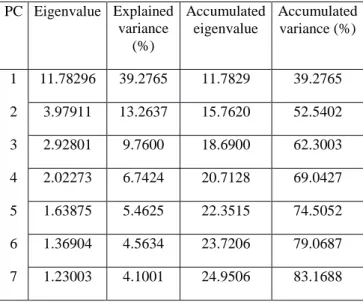
Non-stationary tests such as the ADF test [46] and KPSS test [47] were applied to the original series in levels and then in first differences, showing that the variables T9, T11 , T13, T18, T20, T21, T22, T23, and T29 are non-stationary before running PCA analysis. Therefore, these variables are integrated (d=1 or d=2) and a differencing process must be carried out to make the series stationary. A stationary series is important to obtain stable parameters and enable the model to make accurate predictions. To eliminate the correlation among the variables, PCA is performed in the standardized series using the correlation matrix to extract the PCs. The number of selected PCs, the eigenvalues and the explained variance are presented in Table 1.
The PCs selected were those with eigenvalues greater than 1 [25]. The explained variance of 83% was greater than 70%, and seven PCs were thus obtained to represent the original data.
To find the most highly correlated variables with each PC in order to identify the variable influence in each PC and those most likely to cause instability in the system [26], the factor loadings were used. The most important variables in each PC are shown with own factor loadings in parentheses and only the variables that were statistically significant are displayed.
Table 1 Eigenvalues and percentage of variance
explained with their respective accumulated values for the PC selected.
PC Eigenvalue Explained variance (%) Accumulated eigenvalue Accumulated variance (%) 1 11.78296 39.2765 11.7829 39.2765 2 3.97911 13.2637 15.7620 52.5402 3 2.92801 9.7600 18.6900 62.3003 4 2.02273 6.7424 20.7128 69.0427 5 1.63875 5.4625 22.3515 74.5052 6 1.36904 4.5634 23.7206 79.0687 7 1.23003 4.1001 24.9506 83.1688 PC 1: T6 (0.8701), T7 (0.7789), T8 (0.8728), T16 (0.7219), T17 (0.7391), T26 (0.8535), T27 (0.893856) and T28 (0.883953). PC 2: T5 (0.9070), T15 (0.9152), T19 (0.8998), T25 (0.9195). PC 3: ∆T11 (0.9480); ∆T21 (0.9673). PC 4: ∆T13 (0.9080); ∆T23 (0.8880). PC 5: T10 (0.8995). PC 6: ∆T29 (0.9539). PC 7: T3 (0.9759).
Investigating by means of autocorrelation and autocorrelation partial function in the PCs, we found that they are autocorrelated. An ARIMA model was used to estimate the residuals and then to investigate their volatility. Thus, likewise in this stage, the stationarity of the PCs is tested as mentioned in step 1 before proceeding with the modeling stage.
Finally, a joint ARIMA-GARCH family model was estimated. The joint model of the PC selected is shown in Table 2. The residuals may be useful to evaluate the process by means of residual control [31][49][50] because they are free of correlation and autocorrelation, thus avoiding false alarms. The models presented in Table 2 show significant parameters and white noise residuals. Competing models were estimated and did not produce better results than those presented.
Table 2 Models representing the PC selected to obtain the
residuals that come from the ARIMA-GARCH model estimated using a ML-ARCH (Marquardt) method with normal distribution.
Model 1: PC1–AR (1)
Parameter Coeff. SE z-stat
0.429 0.049 8.597
Variance equation – ARCH (1)
0.384 0.056 6.737
0.844 0.098 8.592
Model 2: ∆ PC2- IMA (1,1)
Coeff. SE z-stat
-0.868 0.042 -20.61 Variance equation - ARCH (1)
0.593 0.055 10.642
0.417 0.128 3.238
Model 3: ∆ PC3 – IMA (1,1)
Coeff. SE z-stat
-0.759 0.0465 -16.307 Variance equation - ARCH (1)
0.280 0.031 8.880 0.663 0.088 7.485 Model 4: PC4 – ARMA (1, 1) Coeff. SE z-stat 0.974 0.028 33.65 -0.850 0.055 -15.29 Variance equation - GARCH (1,1)
0.087 0.045 1.938 0.099 0.043 2.290 0.818 0.066 12.344 Model 5: PC5 – ARMA (1, 1) Coeff. SE z-stat 0.975 0.023 42.143 -0.716 0.057 -12.367 Variance Equation - ARCH (1)
0.376 0.034 11.025 0.768 0.123 6.230 Model 6: PC6 - ARMA(1, 2) Coeff. SE z-stat 0.958 0.028 33.272 -1.157 0.084 -13.741 0.248 0.076 3.271
Variance Equation - ARCH (1)
0.521 0.065 7.942 0.518 0.067 7.731 Model 7: ∆ PC7 – IMA (1,1) Coeff. SE z-stat -0.961 0.010 -91.1708 Variance Equation - GARCH (1,1)
0.438 0.049 8.881
0.542 0.074 7.251
0.131 0.043 3.035
As we know, the first PC comes from the first eigenvalue, i.e., the highest value. Thus, consequently, it has the maximum explained variance. This is important in ordering PCs from high to low values of explained variance. In this way, it is possible to order PC1 to PC7.
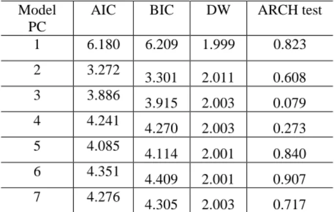
Table 3 shows the adjustment statistics, such as the AIC and BIC, as well as the Durbin-Watson (DW) statistics for the selected models to represent the PCs. The selected model must exhibit a white noise characteristic and the minimum values to AIC and BIC criteria. The ARCH test is used to detect heteroskedasticity. The null hypothesis postulates that there is no heteroskedasticity effect in the series [51].
To confirm the absence of conditional heteroskedasticity in the residuals of the estimated model, the Lagrange multiplier test proposed in Ref. [12] is applied to the final models, where we observed that the residuals were non-heteroskedastic. This was confirmed by the DW test, whose null hypothesis postulates the absence of autocorrelation, showing that the residuals can be considered independent because all the series of major components had values close to 2.0 [35].
Table 3 Statistics of adjustments applied to the residuals
of PCs of the joint ARIMA-GARCH model. Model
PC
AIC BIC DW ARCH test
1 6.180 6.209 1.999 0.823 2 3.272 3.301 2.011 0.608 3 3.886 3.915 2.003 0.079 4 4.241 4.270 2.003 0.273 5 4.085 4.114 2.001 0.840 6 4.351 4.409 2.001 0.907 7 4.276 4.305 2.003 0.717
Note: This table shows data obtained using the AIC, BIC, DW statistics and ARCH test to detect the heteroskedasticity effect, using F(1, 239) chi-square
distribution.
The PCA method was applied to the original data, and the forecasting models were applied to the selected PC. Thus, a new i.i.d. data set is obtained, represented by the residuals from the ARIMA-ARCH model that match the
presuppositions to use control charts and help to evaluate the process stability [52].
To evaluate the stability process, the X-bar and EWMA charts are applied together to capture large and small variations that may affect the production system under study. The parameters set up to build the charts are defined to maintain the same value of ARL = 370. Thus, the charts can be compared. Under these conditions, a range L = 3 is used for the X-bar chart, corresponding to the number of standard deviations. For the EWMA chart, the parameters were set to L = 2.50 standard deviations with a smooth constant of λ = 0.05; both charts use the same subgroup sample size equal to 5.
The run tests, applied to the residuals originating from the PC modeled by the general ARIMA-GARCH model and analyzed using the X-bar chart, assist in characterizing the stability of the process, signaling when a random pattern does not occur. Figures 2-4 show the X-bar, R and EWMA charts of the residuals from the selected PC, fitted by the general ARIMA-GARCH model only for the first PC selected. The others are displayed in Table 4.
The runs test considers three zones: zone A, bounded by three standard deviations from the axis, zone B, the area bounded by two standard deviations from the axis, and zone C, bounded by one standard deviation from the axis, given the X-bar graph.
PC1: Nine subgroup samples on the same side of the
axis, starting at subgroup 2 and ending at 10; 6 subgroup samples in line with growth or decline beginning at subgroup 26 and ending at 34; 2 out of 3 subgroup samples in zone A or beyond, beginning at subgroup 9 and ending at 11; 4 out of 5 subgroup samples in zone B or beyond, beginning at subgroup 8 and ending at 12.
PC2: Two out of 3 subgroup samples in zone A or
beyond, starting at subgroup 37 and ending at 39.
PC3: This PC only shows random variation, without a
special pattern.
PC4: Four out of 5 subgroup samples in zone B or
beyond, starting at subgroup 25 and ending at 29.
PC5: Fourteen subgroup samples alternating above and
below the center line, starting at subgroup 20 and ending at 33; 15 subgroup samples in zone C, beginning at subgroup 27 and ending at 45.
PC6: This PC only shows random variation, without a
special pattern.
PC7: Two out of 3 subgroup samples in zone A or
beyond, beginning at subgroup 9 and ending at 11, and starting at subgroup 12 and ending at 14; 4 out of 5 subgroup samples in zone B or beyond, starting at subgroup 10 and ending at 14.
Fig. 2 X-bar chart for the residuals of the first PC
obtained from an AR(1)- ARCH (1) model.
Fig. 3 R chart for the residuals of the first PC obtained
from an AR(1)- ARCH (1) model.
Fig. 4 EWMA chart for the residuals of the first PC
obtained from an AR(1)-ARCH(1) model.
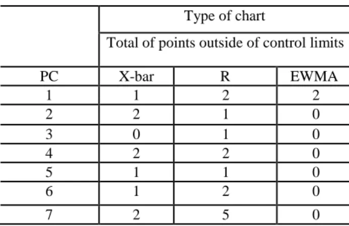
Table 4 presents a summary of the subgroups found to be out-of-control based on X-bar, R and EWMA charts,
applied to the PC residuals. The runs tests and the out-of-control subgroups are helpful in determining the process stability.
Table 4 Subgroup out-of-control limits detected using
X-bar, R and EWMA charts.
Type of chart
Total of points outside of control limits
PC X-bar R EWMA 1 1 2 2 2 2 1 0 3 0 1 0 4 2 2 0 5 1 1 0 6 1 2 0 7 2 5 0
Table 5 shows that the X-bar and R chart capture points outside the control limits of the residuals when analyzing the mean and variability process, respectively. EWMA charts, which are responsible for capturing small variations, detected only small deviations in the first PC. PC1 is the only one showing an out-of-control situation in all charts. The others PCs show an out-of-control situation in at least two charts, except PC3, which is unstable only in the R-chart.
All the situations detected by the runs tests are outlined in Table 5. Only PC1 and PC3 do not show any special characteristics that could be considered as non-random distribution by the runs tests. For example, PC1 and PC7 are the components that present a higher quantity of sequences, which is a sign of possible instability in the process.
When analyzing the volatility reaction coefficient shown by an ARCH model fitted to the PC1, we observe the value 0.8443. This value shows that an external shock to the system takes a long time to make the volatility return to its usual level. Thus, this volatility may affect the variability process, causing an out-of-control situation in the following periods.
Although the residuals of PC2 have points outside the control limits, their volatility reaction, 0.4172, is considered low, which means that an external action may not have a great impact on the productive system.
The EWMA chart reveals that the process is under control, considering small discrepancies from the mean. Thus, external actions that may cause large changes in the process detected by the X-bar chart need to be monitored.
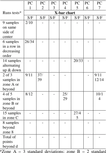
Table 5 Runs tests applied to principal component
residues derived from the joint ARIMA-ARCH model when analyzed using the X-bar chart.
PC 1 PC 2 PC 3 PC 4 PC 5 PC 6 PC 7
Runs tests* X-bar chart
S/F S/F S/F S/F S/F S/F S/F 9 samples on same side of center 2/10 - - - - 6 samples in a row in decreasing order 26/34 - - - - 14 samples alternating up & down - - - - 20/33 - - 2 of 3 samples in zone A or beyond 9/11 37/ 39 - - - 9/11 12/14 4 of 5 samples in zone B or beyond 8/12 - - 25/ 29 10/1 4 15 samples in zone C - - - - 27/4 5 - - 8 samples beyond zone 8 - - - - Total of points beyond d - - - -
*Zone A = 3 standard deviations; zone B = 2 standard deviations; zone C = 1 standard deviation; S = point where the identified sequence starts; and F = point where the identified sequence finishes.
Table 5 reveals only the points outside the control limits of the residuals and a non-random situation in relation to the mean equation. The joint ARIMA-ARCH model is only estimated in combined form because Ref. [53] states that ARCH estimation changes the mean equation specification, as well as the forecasts and the residues behavior. We can see that the PCs were able to maintain all the information of other variables as stated in Ref. [54].
4 CONCLUSION
Statistical process control requires tools for the proper
technology updated following advances in the production process. Thus, an alternative method for control chart evaluation, respecting the necessary conditions, was suggested.
The PCA provides a new uncorrelated data set, resulting in a reduction from 30 to 7 new variables, maintaining high explanatory power over the productive process.
The general ARIMA-GARCH model was able to understand the mean and the volatility behavior in the system. Another important piece of information provided by this joint modeling is the analysis of the volatility persistence, and one external shock to the process could be quantified.
In conclusion, it is important to highlight three important aspects. The first aspect is how to deal with a multivariate process using univariate techniques. Regarding the quality control aspects, our method offered a significant simplification in the parameter estimations and a reduction in the dimension. The second aspect is related to the modeling techniques presented. Although ARIMA-ARCH models are not so straightforward, the parameter estimates using the joint methodology are efficient, providing a better fit to the process. Finally, the ARCH family of models was able quantify the impact of an external effect that can occur in the process. This quantity, represented by the volatility coefficient could be interpreted as a coefficient of reaction in statistical process control.
Further studies are necessary to find new applications in other productive processes as well as for the use of other volatility models.
ACKNOWLEDGEMENTS
The authors are thankful for the financial support of CAPES – Process grants nº BEX-1784/09-9 - CAPES Foundation, Ministry of Education of Brazil. We would also like to thank the ISCTE Business School - Lisbon University Institute for enabling the completion of post-doctoral study. Finally, we are grateful for the financial
support provided by Fundação para a Ciência e Tecnologia (FCT) under the grants #PTDC/GES/73418/2006 and #PTDC/GES/70529/2006. We thanks to the JIMA journal Editor by the cooperation in the final version of this paper.
REFERENCES
[1] Aparisi, F.: “Sampling plans for the multivariate T2 control chart,” Quality Engineering, Vol. 10, No. 1, pp. 141–147 (1997)
[2] Lowry, C.A. and Montgomery, D.C.: “A review of multivariate control charts,” IIE Transactions, Vol. 27, pp. 800–810 (1995)
[3] Tracy, N.D., Young, J.C. and Mason, R.L.: “A practical approach for interpreting multivariate T2 control chart signals,” Journal of Quality Technology, October, Vol. 29, No. 4, pp. 396–406 (1997)
[4] Hawkins, D.M.: “Multivariate quality control based on regression-adjusted variables,” Technometrics, February, Vol. 33, No. 1, pp. 61–75 (1991)
[5] Hawkins, D.M.: “Regression adjustment for variables in multivariate quality control,” Journal of Quality Technology, July, Vol. 25, No. 3, pp. 170–182 (1993)
[6] Timm, N.H.: “Multivariate quality control using finite intersection tests,” Journal of Quality Technology, April, Vol. 28, No. 2, pp. 233–243 (1996)
[7] Souza, A. M. e Rigão, M. H.: “Identificação de variáveis fora de controle em processos produtivos multivariados”, Revista Produção, Vol. 15, No. 1, pp. 074–086, Jan./Abr (2005)
[8] Montgomery, D. C.: Introduction to Statistical Quality Control. 4th Ed., Wiley, New York (2001) [9] Alwan, L. C. and Roberts, H. V.: “Time-series
modeling for statistical process control,” Journal of Business & Economic Statistics, Vol. 6, pp. 87–95 (1988)
[10] Del Castillo, E.: Statistical Control Adjustment for Quality Control. Canadá, John Wiley & Sons, Inc., (2002)
[11] Box, G. E. P. and Jenkins, G. M.: Time series Analysis: Forecasting and Control. San Francisco: Holden-Day (1970)
[12] Engle, R. F.: “Autoregressive conditional heteroskedasticity with estimates of the variance of United Kingdom inflation,” Econometria, Vol. 50, No. 4, pp. 987–1,008 (1982)
[13] Bollerslev, T.: “Generalized autoregressive conditional heteroskedasticity,” Journal of Econometrics, Vol. 31, pp. 307–327 (1986)
[14] Shewhart, W. A.: Economic Control of Quality of Manufactured Product. D. Van Nostrand Company Inc., New York (1931)
[15] Roberts, S.W.: “Control charts tests based on geometric moving averages,” Technometrics, Vol. 1, pp. 239–250 (1959)
[16] Moreira, M. F, in http://www.dalmolim.com.br/EDUCACAO/MATER
IAIS/Biblimat/siderurgia2.pdf acessed on 4th July, 2010
[17] Gujarati, D. N.: Econometria Básica. São Paulo: Makron Books (2000).
[18] Morettin, P. A.; Toloi, C. M. C.: Análise de Séries Temporais. 2nd Ed., São Paulo: Edgard Blücher (2004)
[19] Johnson, R.A.: Wichern, D.W.: Applied Multivariate Statistical Analysis. 3rd Ed. Prentice-Hall. New Jersey (1998)
[20] Luiz J. Corrar, Edilson Paulo e José Maria Dias Filho.: Análise Multivariada para os cursos de Administração, Ciências Contábeis e Economia. Ed. Atlas (2007)
[21] Pearson, K.: “On lines and planes of closed fit to system of point in space,” Phil. Mag., Vol. 6, pp. 559–572 (1901)
[22] Hotelling, H.: “Analysis of a complex of statistical variables into principal components,” The Journal of Educational Psychology, Vol. 24, pp. 417–441/498– 520 (1933)
[23] Morrison, D.F.: Multivariate Statistical Methods. 2nd Ed., Mc Graw Hill, New York (1976)
[24] Seber, G.A.F.: Multivariate Observation. Wiley Series in Probability and Mathematical Statistics. John Wiley and Sons, Inc., New York (1984)
[25] Reinsel, G. C.: Elements of Multivariate Time Series Analysis. Springer-Verlag, New York (1993)
[26] Jackson, J.E.: “Principal components and factor analysis: Part II – additional topics related to principal components,” Journal of Quality Technology, January, Vol. 13. No. 1, pp. 46–58 (1981)
[27] Jackson, J.E.: “Principal components and factor analysis: Part III – what is factor analysis?” Journal
of Quality Technology, April, Vol. 13, No. 2, pp. 125–130 (1981)
[28] Jackson, J. E.: “Principal components and factor analysis: Part I – principal components,” Journal of Quality Technology, October, Vol. 12, No. 4, pp. 201–213 (1981)
[29] Johnson, R. A. and Wichern, D. W.: Applied Multivariate Statistical Analysis. 3rd Ed., Prentice-Hall, New Jersey (1992)
[30] Kaiser H F.: “The application of electronic computers to factor analysis,” Educ. Psychol. Meas. Vol. 20, pp. 141–51 (1960)
[31] Reis, E.: Estatística Multivariada Aplicada, Edições Sílabo. 2nd Ed. (2001)
[32] Mingoti, S. A.: Análise de dados através de métodos de estatística multivariada: uma abordagem aplicada, Editora da UFMG (2005)
[33] Box, G. E. P., Jenkins, G. M. and Reinsel, G. C.: Time Series Analysis: Forecasting and Control. 3rd Ed., Holden-Day, San Francisco (1994)
[34] Makridakis, S. G., Wheelwright, S. C. and Hyndman, R. J.: Forecasting: Methods and Applications. 3rd Ed., John Willey & Sons, Inc., New York (1998)
[35] Morettin, P. A.: Econometria Financeira: um Curso em Séries Temporais Financeiras. São Paulo: Blucher, (2008)
[36] Souza, A. M, Souza, F. M and Menezes, R. M.: “Analysis of equilibrium in industrial variables through error correction models,” International Journal of Academic Research, Vol. 3, No. 1, Part II, January (2011)
[37] Lamounier, M. W.: “Análise da volatilidade dos preços no mercado spot de cafés do Brasil,” Organizações Rurais & Agroindustriais, Lavras, Vol. 8, No. 2, pp. 160–175 (2006)
[38] Jamshidian, F and Zhu, Y.: “Scenario simulation: theory and methodology,” Finance and Stochastics Vol. 1, No. 1, pp. 43–67 (1996)
[39] Costa, P. H. S.; Baidya, T. K. N.: “Propriedades estatísticas das séries de retornos das principais ações brasileiras”, Pesquisa Operacional, Vol. 21, No. 1, pp. 61–87 (2001)
[40] Bentes, S.R., Menezes, R. and Mendes, D. A.: “Long memory and volatility clustering: is the empirical evidence consistent across stock markets?” Physica A. Vol. 387, Issue 15, June (2008)
[41] Campos, K. C.: “Análise da volatilidade de preços de produtos agropecuários no Brasil,” Revista de Economia de Agronegócio, Vol. 5, No. 3, pp. 303– 328 (2007)
[42] Silva, W. S., Sáfadi, T. and Castro Júnior, L. G.: “Uma análise empírica da volatilidade do retorno de commodities agrícolas utilizando modelos ARCH: os casos do café e da soja,” Revista de Economia e Sociologia Rural, Vol. 43, No. 1, pp. 120–134 (2005) [43] Vargas, V. C. C., Lopes, L. F. D. and Souza, A. M.: “Comparative study of the performance of the CUSUM and EWMA control charts,” Computers & Industrial Engineering, Vol. 46, pp. 707–724 (2004) [44] Lucas, M. J. and Saccucci, M.S.: “Exponentially
weighted moving average control schemes: properties and enhancements,” Technometrics, February, Vol. 32. No. 1, pp. 1–12 (1990)
[45] Hunter, J. S.: “The exponentially weighted moving average,” Journal of Quality Technology, Vol. 18, pp. 203–210 (1986)
[46] Western Electric, Statistical Quality Control Handbook. Western Electric Corporation, Indianapolis (1956)
[47] Dickey, D. and Fuller, W.: “Distribution of the estimators for autoregressive time series with a unit root,” Journal of the American Statistical Association, Vol. 84, pp. 427–431 (1979)
[48] Kwiatkowski, D., Phillips, P. C. B., Schmidt, P. and Shin, Y.: “Testing the null hypothesis of stationarity against the alternative of a unit root,” Journal of Econometrics, Vol. 54 (1992)
[49] Box, G.E.P. and Luceño, A.: “Discrete proportional-integral adjustment and statistical process control,” Journal of Quality Technology, July, Vol. 29, No. 3 (1997)
[50] Telhada, M.A.L.: “Cartas de controle multivariadas. Tese de Doutorado,” Escola Politécnica da USP. Engenharia de Produção. [Orientador: José Joaquim do Amaral Ferreira] (1995)
[51] Souza, A. M., Samohyl, R. W. and Malavé, C. O.: “Multivariate feedback control: an application in a productive process,” Computers & Industrial Engineering, Vol. 46, pp. 837–850 (2004)
[52] Soares, I. G.; Castelar, I.,: Econometria aplicada com o uso de EViews, Fortaleza: UFC/CAEN (2003) [53] Requeijo, J. G. e Pereira, Z. L.: “Controlo estatístico em processos com dados auto-correlacionados,” 29º
Colóquio Nacional da Qualidade da APQ, Porto (2004)
[54] Bera, A.K and Higgins, M.L.: “On ARCH models: properties, estimation and testing,” In OXLEY, Les et al. Surveys in Econometrics. Oxford, Blackwell (1995)
[55] Alexander, C.: “Orthogonal methods for generating large positive semi-definite covariances matrices,” Discussion Papers in Finance 2000-06, ISMA Centre (2000)