Printed version ISSN 0001-3765 / Online version ISSN 1678-2690
www.scielo.br/aabc
http://dx.doi.org/10.1590/0001-3765201420130480
Mapping of sites in forest stands
SYLVIO PÉLLICO NETTO, FLAVIO R. STEFANELLO, ALLAN L. PELISSARI and HASSAN C. DAVID
Departamento de Engenharia Florestal, Universidade Federal do Paraná,
Av. Pref. Lothário Meissner, 900, Jardim Botânico, Campus III, 80210-170 Curitiba, PR, Brasil
Manuscript received on December 9, 2013; accepted for publication on March 14, 2014
ABSTRACT
Generally, the forest companies use the total one year planting area as a minimum stratum of the total population and,consequently, the forest inventory processing has been conducted by applying the stratified random sampling to it. This study was carried out in the National Forest of Tres Barras, Brazil, and it aimed to classify and map the sites of Pinus elliottii stands. A systematic sampling was structured into clusters and applied independently by compartments. The clusters, in maltese cross, were composed of four sampling subunits, using Prodansampling method with a fixed number of six trees. By analysis of the methodology it was possible to confirm the hypothesis: a) the selective thinning cause expressive increase of volumetric variability within compartments; b) the variation of sites within the compartments causes volumetric expansion of variance and this grows proportionally to the quality of the sites; c) the stratification in sites results in minimum variance within them; d) the stratification in sites resulted in until to 91% reduction of variances within them.
Key words: Pinus elliottii, Prodan's sampling method, stratification by sites, spatial variation.
Correspondence to: Sylvio Péllico Netto E-mail: [email protected]
INTRODUCTION
The demand for forest products maintains close link with the increase of human population and, as the present expectations, the human population growth rate indicates trends of continuous advance. This fact signals that the forestry sector needs to increase investments in reforestations and improve the quality of products and forest services. With the support and development of new technologies it will become possible
to benefit society directly, by answering the market demand and indirectly, by the decrease of exhaustion
of natural forests.
The forests planted with conifers, today in adult state in Brazil, are derived from projects, in their
majority from fiscal incentive of decades from 1960 to 1980, having its deployment focused more on
quantity of reforested area and little in the quality of the production. In these circumstances, the basic criteria for conducting such plantations were often ignored, which is why it became relevant enhancement
In the literature there are some studies (Tonini et al. 2002, Raulier et al. 2003, Bravo-Oviedo et al. 2004,
Palahi et al. 2004, Rivas et al. 2004, Aertsen et al. 2010, Vargas-Larreta et al. 2010, Kitikidou et al. 2011)
that show, mainly for coniferous forests of the genus Pinus sp., different local qualities, which are indices relating to their potential productivity and obtained in a direct way. Despite the merit and importance of these studies, there are no records documented that such contributions have been complemented with work
relating to mapping of indices of productivity, of fundamental importance as a final process of stratification,
which would allow more accurate information and reliable to forest inventory and, consequently, to the forest management and the planning of production use.
Generally forestry companies adopt an inventory planning, in which only one or two plots are allocated
in each compartment, or one or two plots every twenty five hectares. This spatial sample allocation is adopted due to the cost that data collection represents for the company. By doing so, without detailing the stratification
up to units of site, the sampling estimates do not reach the required standards of precision. On the other hand, if the planning of sampling scheme is performed according to a previous study of the site qualities, this procedure may produce more reliable and more accurate results. In this context, the application of a systematic network of sampling units in the compartments will ensure that all possible productivity classes will be detected by the sampling procedure.
In addition, the companies use the total yearly planted area as a minimum stratum of the total population
- MSP and consequently the forest inventory is conducted by applying strictly the stratified random sampling
up to this level, with total abstention of sample evaluation within the compartments and without detail of
stratification within this MSP.
In the light of the foregoing and aiming to contribute to technical-scientific knowledge on planted
forests, particularly in those of the genus Pinus, this work was conducted to implement the mapping of site classes, which required prior knowledge of site limits at various points in the area selected for this particular experiment. With this purpose, it was appropriate to use a systematic sampling in two stages, with
clusters in the first stage and Prodan’s sampling points with the six nearest trees from a central point in the second stage. Also it was required the site index classification and conclusively the effective mapping of the
sites, which aimed at detection of variability of production in those new strata of the MSP. The objective
of this study was to detect the variability of production, quantified in m3 of woodwith bark per hectare by
compartments, in forest stands of Pinus elliottii Engelm. var. elliottii, to evaluate the appropriateness of
stratification by site.
As hypothesis: 1) The application of selective thinning in compartments of Pinus elliottii var.
elliottii causes significant increase of volumetric variability within them; 2) The variation of sites within
compartments causes volumetric expansion of the variance and this grows proportionally to the quality of
the sites; 3) The stratification of MSP in sites results in minimum variance within them; 4) It will occur expressive volumetric reduction of variance, when the stratification is performed by site units in the MSP.
MATERIALS AND METHODS
STUDY AREA AND DATA COLLECTION
slightly undulated and the soils are of type silty-clayey to clayey, with good water retention capacity and, in general, overly acidic. The vegetation cover is composed of fragments of Mixed Ombrophilous Forest and forest stands of species of the genus Pinus.
Stands of Pinus elliottii var. elliottii were selected for data collection, based on the criterion of larger coverage area of this species inside the limits of that conservation unit,encompassing seven compartments, with a total area of approximately 940 ha and that aimed at identifying variation of existing productivity in the
sites, using a systematic grid of clusters composed of four subunits sampled with the Prodan’s sampling points. The permanent plots or units of fixed area (UFA) were allocated using the simple random sampling,
whose selection obeyed the criterion of randomization of points of the systematic sample network. This
meant that two random selected plots of fixed area always were located at two corresponding sampling units
of the systematic grid. Therefore, two (n) out of twenty five points (C) of the grid were used for the random
sampling, as is commonly made by the companies. For each compartment it was defined a square grid of twenty five clusters, whose structure was organized in accordance with Cochran (1977), Hush et al. (1972) and Sukhatme and Sukhatme (1970).
The systematic sampling was applied indepen dently in each compartment. Their sampling units were
clusters (C) with M subunits (SU). Thus, the population sampled has C clusters, each containing M subunits, in
which i = 1, 2 ... C and j = l, 2 ... M respectively, with the restriction that the number of clusters would be equal in each of the compartments that comprise the forest population to allow a fair comparison of its production. The variable volume (m3), object of analysis, represented by Y
ij, was the value observed in jth cluster, inside the ith
subunit - SU.
The density (n ha-1),of the Prodan’s sampling point was obtained by taking 5.5 trees observed in a
circular variable area until the 6th nearest tree of sample point, computed as half (0.5) tree, by living and at
the same time be the limit of the marginal circle that includes it, as defined by Prodan (1968), Pelz (1983) and Péllico Netto and Brena (1997).
The methodology to calculate the density per hectare, developed by Péllico Netto (1994), was adopted in this study with the purpose of defining the criterion of more precise proportion of participation of the 6th
tree (Ki) in sample subunit (1).
Ki = sen−1(√R26 − r26)(180°R6)−1 (1)
In which: R6 = marginal radius of the sixth tree; and r6 = radius of the cross sectional area of the sixth tree.
The density per subunit (Dij) is obtained by (2)
Dij = 104(5 + Kij)(πR2ij)−1 (2)
The density per cluster (Di) is obtained by (3)
Di = m
Dij 4−1
∑
j−1
(3)
Evaluation of productive capacity and mapping of site unites
Anamorphic curves of site index were constructed by the method of a guide curve, according to Campos
and Leite (2006) and Scolforo (2006), adopting the criterion of dominant height (Hdom) from Assmann,
function of age (I), and fitted to the Prodan’s model (1965), during the elaboration of the management plan
for that conservation unit (Project Flonas Fupef/Ibama 1989) as presented in (4).
(4)
Hdom = I2(β0 + β1I + β2I2)−1 = I2(8.8865 − 0.5303 + 0.0452I2)−1
To describe and model the spatial patterns of site index it was used the geostatistic analysis with the
adjustment of a spherical semivariograma model (Vieira 2000, Andriotti 2003), as presented in (5), and aid of the computer program Geoest (Vieira et al. 2002), with coefficient of determination (R2) of 0.996 and weighted sum of squared deviations (WSSD) equal to 0.0079.
y(h) = C0 + C [1-e(-h
2/A2)
] = 1.6425 + 1.1211 [1-e(-h2/1,9412)
] (5)
where:
y(h) = semivariance, h = distance, C0 = nugget effect, C = sill, and A = range.
The interpolation and the spatialization were performed by ordinary punctual kriging, that considers the spatial dependence and prepare of thematic maps without bias and with minimum variance (Corá and
Beraldo 2006), being drawn up with the program Surfer 9.0, demonstration version (Golden Software 2002), using the limits of dominant heights for site classes at 25 years as reference age.
ESTIMATION OF VOLUMETRIC PRODUCTION
The calculation of volumetric production was performed with the application of the Schumacher-Hall volumetric equation fitted for the species Pinus elliottii var. elliottii in the National Forest of Três Barras,
according to the Final Report of the Project Flonas Fupef/Ibama (1989), as presented in (6).
ln v = β0 + β1ln d + β2ln h = − 9.8618 + 1.8312ln d + 1.0967ln h (6) After the compartment maps were at our disposal, with a network of points properly configured, it was identified the line, the cluster central points (C) and the four points of the subunits (SU). It was identified
the six closest trees to the central point of the four subunits, measured their diameters and heights and the respective distance from this center up to the 6th tree of each (SU). The volume of the (SU) was determined using the volume equation for each tree sampled and performed the summation of individual volumes, except the 6th tree to which it was applied the discount, as is referred in (1).
ADDITIVE LINEAR MODEL APPLIED TO THE EXPERIMENT FOR EVALUATION OF VOLUMETRIC VARIABILITY IN THREE-STAGE HIERARCHICAL STRUCTURE OF SAMPLE
The organization of the Additive Linear Model for application of analysis of variance to a three stages
structure, which characterizes a nested hierarchical model, i.e., the second stage is subordinate to the first
stage and the third stage is subordinate to the second stage, is described below.
The compartments are the primary units (PU), such that i = 1, 2, 3 ... L, in which L is the number of all
compartments that compose the population to be assessed, i.e., there is no sampling in the first stage. Be, subsequently, considered the clusters (C) within the (PU), such that j = 1, 2, 3 ... C, in which C is
pre-fixed, i.e., C = 25 clusters by (PU), not configuring sampling at this stage.
It is considered, by order, the subunits of the clusters (SU), such that k = 1, 2, 3 ... M, in which M is
pre-fixed, i.e. M = 4 subunits in each cluster, also not configuring sampling in this last stage, becoming
As the additive linear model is hierarchical, then it is designed as presented in (7).
Xijk = μ + ai + βj(i) + εk(ji) (7)
From the final composition of the components of variation of the linear model proposed above, the
analysis of variance is presented in Table I.
TABLE I
Structure of the analysis of variance to be applied to the experiment.
Source of Variation Mathematical Expectation Assumptions F Test Compartments (L) S2ε + CM
M ∑ k=1
α2
i(M−1)−1 H
0 : α 2
i = 0 F1 = MQα / MQε Clusters (C) within (L) S2ε + M
C ∑ j=1 M ∑ k=1 β2
j(i)[C(M−1)]−1 H0 : β2j(i) = 0 F2 = MQβ / MQε
Subunits (M) within (C) S2
ε
Total S2x = CM α2i(M−1)−1 + M C ∑ j=1 M ∑ k=1 β2
j(i)[C(M−1)]−1 + S 2
ε
It is worth to clarify that the parameter variance can only be obtained as it is presented in Table I, if the components of variance between primary units and between the clusters exist, i.e., if the null hypotheses are both rejected. In the case of acceptance of the null hypothesis in one or both cases, the variance components are obtained by weighted averages using the appropriate combinations of the mathematical expectations.
By the application of analysis of variance to the experimental data we have: Average of all the subunits in population
X =
L C M
Xijk (NCM)−1
∑ ∑ ∑
i=1 j=1k=1
(8)
Average per subunit in each compartment (PU)
Xi =
C M
Xijk(CM)−1
∑ ∑
j=1k=1
(9)
Average per subunit for each one of the clusters within each primary unit (PU)
Xij =
M
Xijk (M)−1
∑
k=1
(10)
General Variance per subunit
S2
x =
L C M
(Xijk−X)2 (NCM −1)−1
∑ ∑ ∑
i=1 j=1k=1
(11)
By ANOVA, the total variance, under the con dition of rejection of null hypotheses, is obtained by:
(12)
S2x = CM M
∑
k=1α 2
i(M−1)−1+M C
∑
j=1
M
∑
k=1β 2
In that:
S2ε Is the average variance between subunits within the clusters (C) considering all the primary units (PU)
CM
M
∑
k=1α 2
i(M−1)−1 is the variance between the primary units (PU)
M C
∑
j=1 M∑
k=1β 2
j(i)[C(M −1)]−1 is the variance between the means of clusters (C) within the primary units (PU)
Obtaining the Mean Squares in ANOVA
Mean Square between the primary units (PU)
MQe(PU) = CM L
∑
i=1
(Xi−x)2 (N−1)−1 (13)
Mean Square between the clusters within the primary units (PU)
MQe(CG) = M L
∑
i=1 C∑
j=1(Xij − Xi)[N(C−1)]−1 (14)
Mean Square between the subunits of clusters within the primary units (PU)
MQe(SU) = L
∑
i=1 C∑
j=1 M∑
k=1(Xijk − Xij)2 [NC(M−1)]−1 (15)
Variance between the primary units:
CM
M
∑
k=1α 2
i(M−1)−1 =
MQe(UP) − MQe(SU)
CM (16)
Variance between clusters, when the null hypothesis is rejected:
M C
∑
j=1 M∑
k=1β 2
j(i)[C(M−1)]−1 =
MQe(CG) − MQe(SU)
M (17)
And
S2
ε = MQe(SU) (18)
Therefore the total variance can be calculated as follows, in the condition in which both null hypotheses are rejected:
s2
x =
MQe(PU) + C(MQe(CG)) + MQe(SU)[C(M − 1) − 1]
MC (19)
The variance of the mean can be obtained as follows:
(20)
s2x = L−L
CM
M
∑
k=1α 2
i(M−1)−1
+ C−C
M C
∑
j=1 M∑
k=1β 2
j(i)[C(M−1)]−1
+ S
2 ε
L L C LC LCM
As observed, the variance of the mean is reduced only to the value of the variance between the subunits, since the sample fractions do not occurr between compartments and between clusters. It is obtained as follows:
s2
x =
S2ε
The standard deviation can be obtained as follows:
(22)
sx =
r
S2 ε LCM
The coefficient of variation can be obtained as follows:
(23)
cv = sx100
x
The standard error percentage can be obtained as follows:
(24)
sx % =
sx
100
x
The intracluster correlation coefficient can be obtained as follows:
(25)
ρ =
M
C
∑
j=1
M
∑
k=1β 2
j(i)[C(M−1)]−1
M
C
∑
j=1
M
∑
k=1β 2
j(i)[C(M−1)]−1 + S2ε
RESULTS AND DISCUSSION
STATISTICAL TESTS
The population, composed of seven compartments, was stratified according to age, i.e., the compart ments 64, 66 and 67 formed the stratum I (25 years old, in which it was carried out selective thinning) and compartments 76A, 76B, 76C and 76D formed the stratum II (20 years old, before the last thinning). The statistical analyzes is presented in Table II, for of stratification components by age and comparison by "t" test.
Age (year) n Mean (m3ha-1) Variance (m3ha-1)2 Standard Deviation(m3ha-1) Hartley test "t" test
25 (I) 6 458.6 30,301.2 174.1
7.20 * 0.155 ns
20 (II) 8 470.2 4,205.6 64.9
TABLE II
Statistical analyzes applied to fixed area plots measured in seven
compartments allocated into two strata separated by age.
Where: n = number of sample units of fixed area; * = significance level of 5% of probability; and ns = not significant.
As observed in Table II, there was significance at 95% probability between the variances by application of the Hartley' s test, consequently the tabulated value of 't'should be corrected according Cochran and Cox
(1957), i.e.:
t' = w1t1 = w2t2 =(5050.20)(2.571) + (525.70)(2.365)= 14227.3447 = 2.552
w1 = w2 5050.20 + 525.70 5575.90 (26)
where
w1 = s21 1n−1; w2 = s22 2n−1; t1 and t2 are respectively the table values of "t" for n1−1 e n2−1 degrees of freedom.
Still referring to Table II, the application of selective thinning has changed the structure of the population
The reduction of the volumetric stock in stratum I, due to thinning, made it possible an approximation of the volumes in the two strata, which are common in these circumstances, but such an expressive increase of variance explains the reduction of precision when the results of the continuous forest inventories are reported for this species.
For the statistical analysis of the systematic sampling, the population was stratified using the
compartments as administrative strata. Due to the high sampling intensity applied within the compartments it has become important also to analyze the behavior of the variances within them, mainly to assess the
influence of thinning application. Still, this analysis was conducted in two stages: the first was individually
applied within each compartment, with a sample of clusters taken in each compartment, in which the clusters
will detect the spatial variability of volume within them (Tables III and IV) and, in addition, the variability between them (Table V).
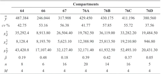
As seen in Table III, the behavior of the total variances (S2T) and the respective estimators of the
intracluster correlation coefficient (ρ) shows the influence of the sites in results of volumetric estimators by
cluster, whose interpretative synthesis is presented in Table IV. These results prove the second hypothesis.
Compartments
64 66 67 76A 76B 76C 76D
y 487.384 246.044 317.908 429.450 430.175 411.196 380.560
cv % 42.75 53.16 56.38 41.77 57.85 55.72 37.56
s2
d 35,292.4 8,913.80 26,504.40 19,782.50 36,119.00 33,282.20 19,484.50
s2e 8,128.4 8,193.70 5,623.10 12,388.90 25,813.50 19,210.80 946.80
s2T 43,420.8 17,107.40 32,127.40 32,171.40 61,932.50 52,493.10 20,431.30
ρ 0.19 0.48 0.18 0.39 0.42 0.37 0.05
n 8 6 16 20 14 16 5
M 4 4 4 4 4 4 4
Where: y = average; cv% = coefficient of variation; s2
d = variance within clusters; s2e= variance
between clusters; s2
T = total variance of clusters; ρ = estimate of the intracluster correlation coefficient;
n = number of clusters sampled; and M = number of Prodan’s sampling points per cluster.
TABLE III
Summary of the intracluster correlation coefficients applied to the
systematic sampling of clusters (C) in each compartment (PU).
Intracluster
correlation coefficient Situation Compartments Evaluation
0.00 - 0.10 Homogeneous within
the compartments 76D A single site
0.10 - 0.20 Semi-homogeneous within
the compartments 67 and 64
Two sites, but with high preponderance of a single site > 0.20 Heterogeneous within
the compartments 66, 76A, 76B and 76C
More than one site and with equitable participation of them in the compartment
TABLE IV
As presented in the methodology, the stratification in three-stage hierarchical design allows you to
evaluate in a global manner throughout the experimental structure. That way, it can test the degree of volumetric homogeneity among compartments and between the clusters within the compartments, whose result is presented in Table V.
Sources of Variation GL SQ MQ F F 5% F 1%
Between compartments 6 3,514,024.75 585,670.79 165.50** 2.12 2.84 Between clusters within compartments 168 1,547,971.31 9,214.11 2.60** 1.22 1.33
Between subunits within clusters 525 1,857,828.10 3,538.72
Total 699 6,919,824.16
TABLE V
Analysis of variance of the systematic sampling stratified by compartments.
Where: ** = significant at 1% of probability level.
As observed in Table V, it has occurred significances at 99% probability level between compartments
and also between the clusters within the compartments. These results clearly show the need to stratify populations by site. As the compartments are administrative units within the MSP, only partially reduces
the total variance, remaining the variation due to the sites. In the same way, the high significance observed
among the clusters within the compartments portrays the heterogeneity due to the sites.
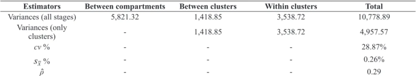
Estimators Between compartments Between clusters Within clusters Total
Variances (all stages) 5,821.32 1,418.85 3,538.72 10,778.89
Variances (only
clusters) - 1,418.85 3,538.72 4,957.57
cv % - - - 28.87%
sx % - - - 0.26%
ρ - - - 0.29
TABLE VI
Statistics of the sampled population.
Where: cv % = coefficient of variation; sx % = standard error percentage; and ρ = estimate of the intracluster correlation coefficient.
TABLE VII
Analysis of variance for site classes with systematic sampling.
Strata
N s2
e s
2
d s
2 T
s2T
Media F ρ
Age (year) Site classes
25 III 31 719.8 1,064.0 1,783.7 2,498.0 3.71 * 0.404
IV 43 1,482.2 1,730.0 3,212.3 4.43 * 0.461
20 II 90 378.5 451.6 830.1 787.1 4.35 * 0.456
III 11 331.8 412.4 744.1 4.22 * 0.446
Where: s2
e = variance between clusters; s 2
d = variance within clusters; s 2
T = total variance of clusters; F = variance ratios to test hypothesis of means; ρ = estimate of the intracluster correlation coefficient; N = number of clusters; and
* significance at 5% probability.
For better understanding of these results of the ANOVA, a synthesis of the statistics is presented in Table VI.
which caused approximation of the volumetric means at both ages (25 and 20 years). The precision of this sampling design, of the order of 0.26%, occurred by the high intensity of clusters sampled in each compartment (25 units) and also because the ANOVA model, composed of fixed effects in the first two levels of stratification, enables the calculation of standard error in percentage only as function of the variance within clusters. The intracluster correlation coefficient (0.29) shows once more the heterogeneity among the clusters, i.e., the variability of the clusters’ means within the compartments, of the order of 30% of their total variability, corresponds to the average value of the intracluster correlation coefficients
calculated independently within each compartment, as shown in Table III.
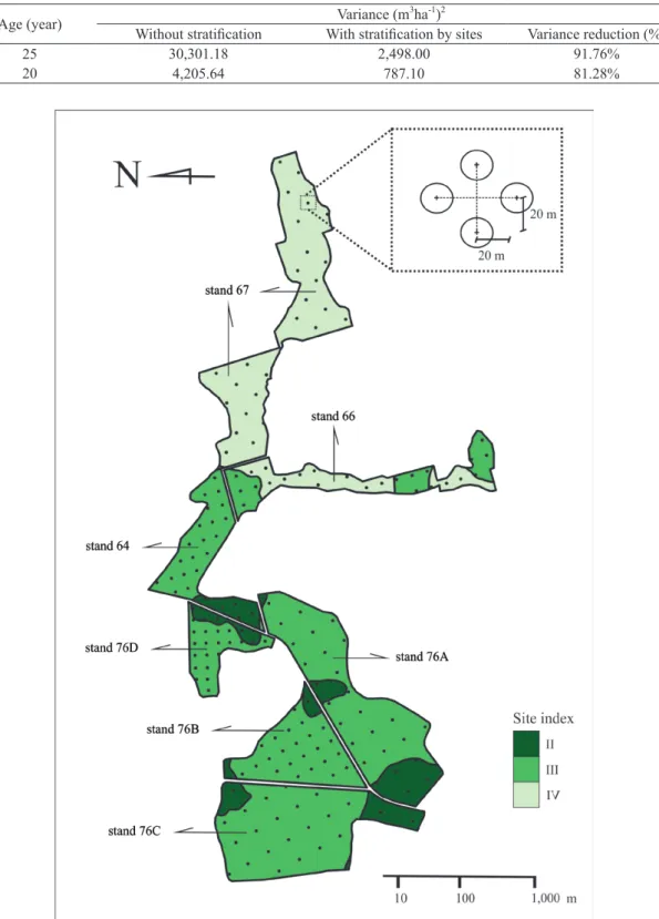
MAPPING OF CLASSES OF SITE
With the objective of checking if the stratification in sites in the population results statistical significance,
the mapping of site index classes was performed at the level of compartments, that is, the population refers
to the sum of them (Figure 1).
The analysis of variance was conducted using only the clusters within the sites and also separated by
age, exactly to keep one year of planting as the basic unit for stratification. This adopted procedure for the analysis of variance was described by Ostle and Mensing (1975) (Table VII).
As seen in Table VII, we proved what was formulated in the third hypothesis, because there was significant
reduction of the variance on volume, when the clusters were processed only within each unit of site, the new
stratification procedure within the EMP. The mean variance in the age of 25 years is kept higher than that at
the age of 20 years, due to the application of selective thinning in the older stands.
The results of the ANOVA showed that remains significance at 95% probability among the clusters within the strata, expressed by the uniformity of the intracluster correlation coefficient in all of them, showing that their total variances comprise approximately 45% between clusters and 55% within them.
These results are attributed to the occurrence of uneven density within sites, whether by effect of thinning in stands of 25 years, or by mortality in stands of 20 years.
SYSTEMATIC VERSUS RANDOM SAMPLING
The comparison of the results obtained by applying the two sampling procedures is presented in Table VIII.
Compartments Random Sampling (plots) Systematic Sampling (clusters) Volume (m3ha-1) Total Production (m3) Volume (m3ha-1) Total Production (m3)
64 638.123 14,893.800 487.384 1,375.530
66 295.565 8,000.940 246.044 6,660.320
67 442.104 22,503.070 317.908 16,183.170
76A 493.513 27,819.340 429.450 24,101.540
76B 472.101 13,596.500 430.175 12,353.280
76C 458.068 25,935.780 411.196 23,281.970
76D 456.957 7,146.800 380.560 5,952.560
Mean* /Total 414.190 107,168.000 389.865 100,874.000
IC Mean/Total ** ± 66.490 ± 17,202. 000 ± 1.014 ± 262.272
TABLE VIII
Comparison of average and total production by compartments with random sampling (plots) and systematic sampling (clusters).
TABLE IX
Comparison of the variances of the variable volume
obtained without and with stratification by sites.
Age (year) Without stratification With stratification by sitesVariance (m3ha-1)2 Variance reduction (%)
25 30,301.18 2,498.00 91.76%
20 4,205.64 787.10 81.28%
Figure 1 - Geographical location of the cluster units in a systematic pattern and identification
The large increase in precision obtained in the application of clusters was due to greater coverage in the detection of internal variability in the compartments and the high sampling intensity applied (25 clusters with
four subunits each, totaling 100 subunits in each compartment and 700 in all compartments), compared with 14 units of plots used in the random sampling (two plots per compartment).
Conclusively, the comparison of variances obtained by the two procedures used in this study, the
traditional one used by companies and the stratification by sites, is synthesized in Table IX.
As seen in Table IX, the reductions of variances by application of stratification by sites has reached 91.76 %, occurred in stands with 25 years and 81.28% for the stands of 20 years. Such results are very
expressive and prove the fourth hypothesis formulated in this work.
To improve the structure of continuous forest inventories in the companies and significantly increase of the precision of sampling estimators, it is strongly recommended the stratification by production sites in the MSP.
RESUMO
Geralmente as empresas florestais usam a área total de um ano de plantio como estrato mínimo do total da população e, consequentemente, o processamento do inventário florestal tem sido realizado pela aplicação da amostragem aleatória estratificada. Este estudo foi realizado na Floresta Nacional de Três Barras, Brasil, e teve como objetivo classificar e mapear os locais onde Pinus elliottii se destaca. A amostragem sistemática foi estruturada em grupos e aplicada de forma independente por compartimentos. Os conglomerados em cruz maltesa, foram compostos por quatro subunidades de amostragem, utilizando o método de amostragem Prodan com um número fixo de seis árvores. Pela análise da metodologia, foi possível confirmar as hipóteses: a) o afinamento seletivo causa expressivo aumento de variabilidade volumétrica dentro dos compartimentos; b) a variação de locais no interior dos compartimentos provoca a expansão volumétrica de variância e esta cresce proporcionalmente à qualidade dos sítios; c) a estratificação em locais resulta em menor variância dentro deles; d) a estratificação em locais resultou em redução de até 91% das variâncias dentro deles.
Palavras-chave: Pinus elliottii, amostragem de Prodan, estratificação por sítios, variabilidade espacial.
REFERENCES
AERTSEN W, KINT V, VAN ORSHOVEN J, ÖZKAN K AND MUYS B. 2010. Comparison and ranking of different modeling techniques for prediction of site index in Mediterranean mountain forests. Ecol Model 221: 1119-1130.
ANDRIOTTI JLS. 2003. Fundamentos de estatística e geoestatística, São Leopoldo, 165 p.
BRAVO-OVIEDO A, RIO MD AND MONTERO G. 2004. Site index curves and growth model for Mediterranean maritime pine (Pinus pinaster Ait.) in Spain. For Ecol Manage 201: 187-197.
CAMPOS JCC AND LEITE HG. 2006. Mensuração florestal, 2a ed., Viçosa, 470 p.
COCHRAN WG. 1977. Sampling techniques.3rd ed., New York, J Wiley & Sons, Inc., 428 p.
COCHRAN WG AND COX GM. 1957. Experimental Design, 2nd ed., New York, J Wiley & Sons, Inc., 611 p.
CORÁ JE AND BERALDO JMG. 2006. Spatial variability of soil properties before and after lime and phosphorus fertilizer application
at variable rates in sugarcane. Eng Agric 26(2): 374-387.
GOLDEN SOFTWARE. 2002. Surfer: user’s guide, Colorado, Golden Software, 664 p.
HUSH B, MILLER CI AND BEERS TW. 1972. Forest mensuration,2nd ed., New York, The Ronald Press Company, 410 p.
KITIKIDOU K, BOUNTIS D AND MILIOS E. 2011. Site index models for calabrian pine (Pinus brutia Ten.) in Thasos Island, Greece.
Cienc Flor 21(1): 125-131.
OSTLE B AND MENSING RW. 1975. Statistics in research.3rd ed., Iowa, The Iowa State University Press, 596 p.
PALAHI M, TOME M, PUKKALAC T, TRASOBARES A AND MONTEROD G. 2004. Site index model for Pinus sylvestris in north-east Spain. For Ecol Manage 187: 35-47.
PÉLLICO NETTO S. 1994. Correction factor for marginal trees in sampling methods with probabilistic selection proportional to a
size. Cerne 1(1): 17-27.
PELZ DR. 1983. Sixth-tree sampling in forest inventories. Floresta 14(1): 54-58.
PRODAN M. 1965. Holzmesslehre,Franfurt, J.D. Sauerländer’s Verlag, 644 p.
PRODAN M. 1968. Punktstichprobe für die forsteirichtung. Forst U Holzwirt23(11): 225-226.
PROJECT FLONA FUPEF/IBAMA. 1989. Inventário de Florestas Plantadas da Floresta Nacional de Três Barras/SC, Curitiba. RAULIER F, LAMBERT M, POTHIER D AND UNG C. 2003. Impact of dominant tree dynamics on site index curves. For Ecol Manage
184: 65-78.
RIVAS JJC, GONZÁLEZ JGA, GONZÁLEZ ADR AND GADOW KVON. 2004. Compatible height and site index models for five pine species in El Salto, Durango (Mexico). For Ecol Manage 201: 145-160.
SCOLFORO JRS. 2006. Biometria florestal: modelos de crescimento e produção florestal. Lavras, 393 p.
SUKHATME PV AND SUKHATME DL. 1970. Sampling theory of surveys with applications. 2nd ed., Ames, Iowa, Iowa State University Press, 452 p.
TONINI H, FINGER CAG, SCHNEIDER PR AND SPATHELF P. 2002. Graphical comparison among site index curves for Pinus elliottii and Pinus taeda, built at south Brazil. Cienc Flor 12(1): 143-152.
VARGAS-LARRETA B, ÁLVAREZ-GONZÁLEZ JG, CORRAL-RIVAS JJ AND AGUIRRE-CALDERÓN ÓA. 2010. Development of dynamic site index curves for Pinus cooperi blanco. Rev Fitotec Mex 33(4): 343-351.
VIEIRA SR. 2000. Geostatistics in soil spatial variability studies. In: NOVAIS RF, ALVAREZ VVH AND SCHAEFER CEGR (Eds), Topics in soil science, Brazilian Society for Soil Science, Viçosa, p. 1-54.