P ´
OS-GRADUAC
¸ ˜
AO EM ENGENHARIA EL´
ETRICA
A NOVEL WORD BOUNDARY
DETECTOR BASED ON THE TEAGER
ENERGY OPERATOR FOR AUTOMATIC
SPEECH RECOGNITION
IGOR SANTOS PERETTA
UBERL ˆ
ANDIA
IGOR SANTOS PERETTA
A NOVEL WORD BOUNDARY
DETECTOR BASED ON THE TEAGER
ENERGY OPERATOR FOR AUTOMATIC
SPEECH RECOGNITION
Disserta¸c˜ao apresentada ao Programa de P´os-Gradua¸c˜ao em Engenharia El´etrica da Universidade Federal de Uberlˆandia, como requisito parcial para a obten¸c˜ao do t´ıtulo de Mestre em Ciˆencias.
´
Area de concentra¸c˜ao: Processamento da Informa¸c˜ao, Inteligˆencia Artificial
Orientador: Prof. Dr. Keiji Yamanaka
UBERL ˆ
ANDIA
, &+ . +
/ . 0 1 2 ' 3 +
' 4 5 ! 6 5 7
' 8 9 ' : $ : ; +
& +
+ < $ ' '= ! > ? + ,+ < &
? + + 2 ' 3 0 1 + + 5 ! 6 5 7 +
' 8 9 ' : $ : ; + + ?@ +
IGOR SANTOS PERETTA
A NOVEL WORD BOUNDARY
DETECTOR BASED ON THE TEAGER
ENERGY OPERATOR FOR AUTOMATIC
SPEECH RECOGNITION
Disserta¸c˜ao apresentada ao Programa de P´os-Gradua¸c˜ao em Engenharia El´etrica da Univer-sidade Federal de Uberlˆandia, como requisito parcial para a obten¸c˜ao do t´ıtulo de Mestre em Ciˆencias.
´
Area de concentra¸c˜ao: Processamento da In-forma¸c˜ao, Inteligˆencia Artificial
Uberlˆandia, 21 de dezembro de 2010
Banca Examinadora
Keiji Yamanaka, PhD - FEELT/UFU
Hani Camille Yehia, PhD - DELT/UFMG
Gilberto Carrijo, PhD - FEELT/UFU
companheirismo. `
Agradecimentos
`
A minha esposa Anabela e `a minha filha Isis, pelo amor, suporte, carinho e compreens˜ao durante esta complicada fase de dedica¸c˜ao `a minha pesquisa. Aos meus pais, Vitor e Miriam, e aos meus irm˜aos, ´Erico e ´Eden, pelo amor e apoio incondicionais e por sempre acreditarem em mim.
Ao meu orientador, Prof. Dr. Keiji Yamanaka, pela confian¸ca em mim depositada, pela presteza em auxiliar e pela grande oportunidade de traba-lharmos juntos.
Aos meus companheiros em armas, Gerson Fl´avio Lima e Josimeire Tavares, pela amizade, companhia constante e pelos trabalhos realizados.
Ao Prof. Dr. Jos´e Roberto Camacho, pelas conversas, conhecimentos compartilhados e pelo espa¸co cedido para este trabalho.
Ao Prof. Dr. Shigueo Nomura, pelo suporte, an´alises e longas conversas. Aos Prof. Dr. Gilberto Carrijo e Profa. Dra. Edna Flores, pelos conhe-cimentos compartilhados.
Ao Prof. Dr. Hani Camille Yehia, pelas considera¸c˜oes e contribui¸c˜oes inestim´aveis.
Aos companheiros Eduardo, Marlus, Mattioli e F´abio, pela amizade, pelo caf´e e pela ajuda imprescind´ıvel em momentos cr´ıticos.
Aos companheiros de laborat´orio, em especial a ´Elvio, Fabr´ıcio e Fer-nando, pelas conversas, aux´ılios e amizade.
Aos amigos Maria Estela Gomes, Pedro Paro, Edna Coloma e L´ucia Mansur, pelo apoio inigual´avel. Muito obrigado!
Aos amigos que deixei na DGA da Unicamp, pelo carinho, suporte e pelos momentos juntos. Em especial a Talita, Elza, Soninha, Renata, Marli, Angela, Serginho, Adagilson, Regina, Rozi, Ivone, Zanatta, Nanci, Pedro Henrique e Felipe.
Aos amigos de Campinas, Daltra & Dani, Barb´a e Peri, pelas longas e saudosas conversas. `A fam´ılia S´ergio, Leandra, Miguel e Gabriela e `a fam´ılia Loregian, Fabiana e Tain´a, pela amizade sincera.
Aos amigos de infˆancia Carlos Augusto Dagnone e Marco Antˆonio Zanon Prince Rodrigues, pela longa amizade e pela caminhada que trilhamos juntos.
“We are all apprentices in a craft where no one ever becomes a master.”
(ERNEST HEMINGWAY, 1961)
“Somos todos aprendizes em um of´ıcio no qual ningu´em nunca se torna mestre.”
Este trabalho ´e parte integrante de um projeto de pesquisa maior e con-tribui no desenvolvimento de um sistema de reconhecimento de voz inde-pendente de locutor para palavras isoladas, a partir de um vocabul´ario limi-tado. O presente trabalho prop˜oe um novo m´etodo de detec¸c˜ao de fronteiras da palavra falada chamado “M´etodo baseado em TEO para Isolamento de Palavra Falada”(TSWS). Baseado no Operador de Energia de Teager (TEO), o TSWS ´e apresentado e comparado com dois m´etodos de segmenta¸c˜ao da fala amplamente utilizados: o m´etodo “Cl´assico”, que usa c´alculos de ener-gia e taxa de cruzamento por zero, e o m´etodo “Bottom-up”, baseado em conceitos de equaliza¸c˜ao de n´ıveis adaptativos, detec¸c˜ao de pulsos de energia e ordena¸c˜ao de limites. O TSWS apresenta um aumento na precis˜ao na de-tec¸c˜ao de limites da palavra falada quando comparado aos m´etodos Cl´assico (redu ¸c˜ao para 67,8% do erro) e Bottom-up (redu¸c˜ao para 61,2% do erro).
Um sistema completo de reconhecimento de palavras faladas isoladas (SRPFI) tamb´em ´e apresentado. Este SRPFI utiliza coeficientes de Mel-Cepstrum (MFCC) como representa¸c˜ao param´etrica do sinal de fala e uma rede feed-forward multicamada padr˜ao (MLP) como reconhecedor. Dois conjuntos de testes foram conduzidos, um com um banco de dados de 50 palavras diferentes com o total de 10.350 pron´uncias, e outro com um vo-cabul´ario menor — 17 palavras com o total de 3.519 pron´uncias. Duas em cada trˆes dessas pron´uncias constituem o conjunto para treinamento para o SRPFI, e uma em cada trˆes, o conjunto para testes. Os testes foram conduzidos para cada um dos m´etodos TSWS, Cl´assico ou Bottom-up, uti-lizados na fase de segmenta¸c˜ao da fala do SRPFI. O TSWS permitiu com que o SRPFI atingisse 99,0% de sucesso em testes de generaliza¸c˜ao, contra 98,6% para os m´etodos Cl´assico eBottom-up. Em seguida, foi artificialmente adicionado ru´ıdo branco gaussiano `as entradas do SRPFI para atingir uma rela¸c˜ao sinal/ru´ıdo de 15dB. A presen¸ca do ru´ıdo alterou a performance do SRPFI para 96,5%, 93,6% e 91,4% em testes de generaliza¸c˜ao bem sucedidos quando utilizados os m´etodos TSWS, Cl´assico eBottom-up, respectivamente.
ix
Palavras-chave
This work is part of a major research project and contributes into the development of a speaker-independent speech recognition system for isolated words from a limited vocabulary. It proposes a novel spoken word boundary detection method named “TEO-based method for Spoken Word Segmenta-tion” (TSWS). Based on the Teager Energy Operator (TEO), the TSWS is presented and compared with two widely used speech segmentation me-thods: “Classical”, that uses energy and zero-crossing rate computations, and “Bottom-up”, based on the concepts of adaptive level equalization, energy pulse detection and endpoint ordering. The TSWS shows a great precision improvement on spoken word boundary detection when compared to Clas-sical (67.8% of error reduction) and Bottom-up (61.2% of error reduction) methods.
A complete isolated spoken word recognition system (ISWRS) is also presented. This ISWRS uses Mel-frequency Cepstral Coefficients (MFCC) as the parametric representation of the speech signal, and a standard multi-layer feed-forward network (MLP) as the recognizer. Two sets of tests were conducted, one with a database of 50 different words with a total of 10,350 utterances, and another with a smaller vocabulary — 17 words with a total of 3,519 utterances. Two in three of those utterances constituted the train-ing set for the ISWRS, and one in three, the testtrain-ing set. The tests were conducted for each of the TSWS, Classical or Bottom-up methods, used in the ISWRS speech segmentation stage. TSWS has enabled the ISWRS to achieve 99.0% of success on generalization tests, against 98.6% for Classi-cal and Bottom-up methods. After, a white Gaussian noise was artificially added to ISWRS inputs to reach a signal-to-noise ratio of 15dB. The noise presence alters the ISWRS performances to 96.5%, 93.6%, and 91.4% on generalization tests when using TSWS, Classical and Bottom-up methods, respectively.
xi
Keywords
Contents xiii
List of Figures xv
List of Tables xvii
List of Algorithms xx
1 Introduction 1
1.1 Overview . . . 1
1.2 Motivation . . . 3
1.3 Database . . . 4
2 State of Art 6 2.1 Speech Segmentation . . . 7
2.2 Feature Extraction . . . 9
2.2.1 Human Sound Production System Based Models . . . . 10
2.2.2 Human Auditory System Based Models . . . 12
2.3 Speech Recognition . . . 16
2.4 Choices for this Work . . . 20
3 Theoretical Background 21 3.1 Audio Signal Capture . . . 22
3.2 Preprocessing . . . 23
3.2.1 Offset compensation . . . 23
3.2.2 Pre-emphasis filtering . . . 24
3.3 Speech Segmentation . . . 24
3.3.1 The Teager Energy Operator . . . 25
CONTENTS xiii
3.4 Feature Extraction . . . 26
3.5 The Recognizer . . . 30
3.5.1 Confusion Matrices . . . 33
4 Proposed Method for Speech Segmentation 35 4.1 Support Database . . . 36
4.2 Proposed TEO-Based Segmentation . . . 37
4.3 TSWS Experimental Results . . . 45
4.4 Extended Comparison between Methods . . . 55
5 Experimental Results 60 5.1 Training and Testing Patterns . . . 60
5.2 Results from Project Database . . . 61
5.3 Smaller Vocabulary . . . 65
5.3.1 Confusion Matrices for 17 Words Vocabulary . . . 69
5.3.2 Confusion Matrices for 17 Words Vocabulary with SNR 15dB . . . 73
6 Conclusion 77 6.1 Main Contribution . . . 78
6.2 Ongoing Work . . . 79
6.3 Publications . . . 80
References 82 Appendix 93 A Compton’s Database 93 B TSWS C++ Class: Source Code 98 B.1 Header . . . 100
B.2 Code . . . 100
2.1 Three utterances from the same speaker for the word OPC¸ ˜OES /op"s˜oyZ/. . . 9
3.1 Proposed speech recognition system block diagram. . . 22 3.2 Overlapping of windows on frames for coefficient evaluation. . 27 3.3 Hertz scale versus Mel scale. . . 28 3.4 Filters for generating Mel-Frequency Cepstrum Coefficients. . 30 3.5 Diagram with a I×K×J MLP acting as recognizer. . . 31 3.6 A Perceptron with the hyperbolic tangent as the activation
function. . . 32
4.1 Audio waveform for the English word “HOT” /hat/ with white noise addition (SNR 30dB). . . 38 4.2 Audio waveform for the English word “HOT” /hat/ from
sup-port database with white noise addition (SNR 30dB), and re-spective boundary found by the TSWS method, with A= 9. . 40 4.3 Proposed word boundary detection algorithm (flowchart). . . . 41 4.4 Audio waveform for the English word “CHIN” /tSIn/,
tar-get manually positioned boundary, and respective boundaries found by TSWS, Classical and Bottom-up methods. . . 46 4.5 Estimator curve for empirical SNR-dependent constantA. . . 48 4.6 RMSE per phoneme type for TSWS (A = 25), Classical and
Bottom-up methods, with clear signals. . . 51 4.7 RMSE per phoneme type for TSWS (A = 9), Classical and
Bottom-up methods, with SN R = 30dB. . . 52 4.8 RMSE per phoneme type for TSWS (A = 3), Classical and
Bottom-up methods, with SN R = 15dB. . . 53 4.9 RMSE per phoneme type for TSWS (A = 1.1), Classical and
Bottom-up methods, with SN R = 5dB. . . 54
LIST OF FIGURES xv
5.1 Comparison of the training set successful recognition rates, in %, for MFCC-MLP-recognizer using TSWS, Classical and Bottom-up methods. . . 63 5.2 Comparison of the testing set successful recognition rates,
in %, for MFCC-MLP-recognizer using TSWS, Classical and Bottom-up methods. . . 64 5.3 Comparison of the testing set successful recognition rates in %
for MFCC-MLP-recognizer using TSWS, Classical and Bottom-up methods with smaller vocabulary. . . 67 5.4 Comparison of the training set successful recognition rates
in % for MFCC-MLP-recognizer using TSWS, Classical and Bottom-up methods, with addition of WGN to achieve a SNR of 15dB. . . 68 5.5 Comparison of the testing set successful recognition rates in %
1.1 Parameters used to characterize speech recognition systems . . 3 1.2 Brazilian Portuguese voice commands from the project database. 5
3.1 Proposed speech recognition system . . . 21 3.2 Center frequencies and respective bandwidth for the designed
16 triangular bandpass filters. . . 29
4.1 Time parameters (constants) for the TSWS algorithm. . . 41 4.2 Empirical SNR-dependent constantAfrom the TSWS method
against SNR. . . 48 4.3 Overall RMSE (in milliseconds) from TSWS, Classical, and
Bottom-up segmentation methods. . . 49 4.4 Support database (Clear signal) comparison of TSWS (A =
25) with Classical and Bottom-up methods. . . 56 4.5 Modified support database (SN R = 30dB) comparison of
TSWS (A= 9) with Classical and Bottom-up methods. . . 57 4.6 Modified support database (SN R = 15dB) comparison of
TSWS (A= 3) with Classical and Bottom-up methods. . . 58 4.7 Modified support database (SN R = 5dB) comparison of TSWS
(A= 1.1) with Classical and Bottom-up methods. . . 59
5.1 Overall successful recognition rates (in %) for MFCC-MLP-recognizer. . . 61 5.2 Worse TSWS supported individual recognition rates (RR), in
%, when compared to Classical and Bottom-up (CL/BU) me-thods. . . 62 5.3 Better TSWS supported individual recognition rates (RR), in
%, when compared to Classical and Bottom-up (CL/BU) me-thods. . . 63 5.4 Portuguese voice commands from the smaller vocabulary. . . . 65
LIST OF TABLES xvii
5.5 Overall successful recognition rates in % for MFCC-MLP-recognizer with a vocabulary of 17 words. . . 66 5.6 Overall successful recognition rates in % for
MFCC-MLP-recognizer with a vocabulary of 17 words and SNR of 15dB. . 67 5.7 Confusion matrix fortraining set using TSWS andMel-Cepstral
Coefficients [Clear signals] with rates in %. Overall recogni-tion rate of 100.0%. . . 70 5.8 Confusion matrix fortesting set using TSWS andMel-Cepstral
Coefficients [Clear signals] with rates in %. Overall recogni-tion rate of 99.0%. . . 70 5.9 Confusion matrix for training set using Classical and
Mel-Cepstral Coefficients [Clear signals] with rates in %. Overall recognition rate of 100.0%. . . 71 5.10 Confusion matrix fortesting setusingClassical andMel-Cepstral
Coefficients [Clear signals] with rates in %. Overall recogni-tion rate of 98.6%. . . 71 5.11 Confusion matrix for training set using Bottom-up and
Mel-Cepstral Coefficients [Clear signals] with rates in %. Overall recognition rate of 100.0%. . . 72 5.12 Confusion matrix for testing set using Bottom-up and
Mel-Cepstral Coefficients [Clear signals] with rates in %. Overall recognition rate of 98.6%. . . 72 5.13 Confusion matrix fortraining set using TSWS andMel-Cepstral
Coefficients [SNR 15dB] with rates in %. Overall recognition rate of 100.0%. . . 74 5.14 Confusion matrix fortesting set using TSWS andMel-Cepstral
Coefficients [SNR 15dB] with rates in %. Overall recognition rate of 96.5%. . . 74 5.15 Confusion matrix for training set using Classical and
Mel-Cepstral Coefficients [SNR 15dB] with rates in %. Overall recognition rate of 99.8%. . . 75 5.16 Confusion matrix fortesting setusingClassical andMel-Cepstral
Coefficients [SNR 15dB] with rates in %. Overall recognition rate of 93.6%. . . 75 5.17 Confusion matrix for training set using Bottom-up and
Mel-Cepstral Coefficients [SNR 15dB] with rates in %. Overall recognition rate of 99.9%. . . 76 5.18 Confusion matrix for testing set using Bottom-up and
List of Algorithms
3.1 Setting frame and window sizes. . . 27
4.1 Proposed TSWS algorithm (pseudocode) - part 1/3 . . . 42
4.2 Proposed TSWS algorithm (pseudocode) - part 2/3 . . . 43
4.3 Proposed TSWS algorithm (pseudocode) - part 3/3 . . . 44
Introduction
1.1
Overview
Speech interface to machines is a subject that has fascinated the
hu-mankind for decades. Let us put aside magical entities that respond to
spoken commands like the Golem in Jewish tradition, or even the entrance of the cave in the Ali Baba and the Forty Thieves Arabic tale. In modern literature, we can track down to L. Frank Baum’s Tik-Tok mechanical man from Ozma of Oz (1907) as the first machine that reacts to human spoken language. Recently, movies like 2001: A Space Odyssey (1968) to the new releasedIron Man (2008) andIron Man II (2010) present us with computers that can comprehend human speech – HAL and JARVIS, respectively.
Engineers and scientists have been researching spoken language interfaces
for almost six decades1. In addition to being a fascinating topic, speech
inter-faces are fast becoming a necessity. Advances in this technology are needed to
1
We could detach the work of Davis, Biddulph and Balashek [15] as one of the first speech recognition systems.
1.1 Overview 2
enable the average citizen to interact with computers, robots, networks, and
other technological devices using natural communication skills. As stated
by Zue and Cole [74], “without fundamental advances in user-centered
in-terfaces, a large portion of society will be prevented from participating in
the age of information, resulting in further stratification of society and tragic
loss of human potential”. They also stated: “a speech interface, in a user’s
own language, is ideal because it is the most natural, flexible, efficient, and
economical form of human communication”.
Several different applications and technologies can make use of spoken
input to computers. The conversion of a captured acoustic signal to a single
command or a stream of words is the top of mind application for speech
recog-nition, but we can also have applications for speaker’s identity recogrecog-nition,
language spoken recognition or even emotion recognition.
After many years of research, speech recognition technology is generating
practical and commercial applications. Some examples for English speech
recognition could be found: Dragon Naturally Speaking; Project54 system;
TAPTalk module; IBM ViaVoice; Microsoft SAPI among others. For
Por-tuguese language, some commercial and freeware solutions are available. But,
the common sense is that speech recognition softwares still roughly work as
desired.
Why is so hard to reach an ultimate solution for speech recognition?
Some languages are easier to reach an acceptable margin of successful
recog-nition rates than others. Applications with smaller vocabulary size could
perform better than large vocabulary ones. But, even solutions with
ac-ceptable recognition rates easily drop their rates down when immersed in
high noise environments. Speaker-independent systems hardly contemplate
enough diversification of utterances. Even speaker-dependent softwares have
dis-order. The main reason is science still does not understand the full process
of hearing: how exactly our brain translates acoustic signals to information
after preprocessing of inner ear; how can we focus in a determined acoustic
source in detriment of others; or even how do we easily understand corrupted
acoustic information inside a familiar context. Those answers could not be
provided, as far as we have searched for them.
1.2
Motivation
Table 1.1, extracted from Zue, Cole and Ward [75], shows the typical
parameters used to characterize speech recognition systems.
Table 1.1: Parameters used to characterize speech recognition systems
Parameters Range
Speaking Mode Isolated words to continuous speech Speaking Style Read speech to spontaneous speech
Enrollment Speaker-dependent to Speaker-independent Vocabulary Small (<20 words) to large (> 20,000 words) Language Model Finite-state to context-sensitive
Perplexity Small (<10) to large (>100)
SNR High (> 30 dB) to low (< 10 dB)
Transducer Voice-canceling microphone to telephone
This work is part of a research that aims to develop a speaker-independent
speech recognition system for recognition of spontaneous spoken isolated
words, with a not so small vocabulary, that could be embedded to several
possible applications. This research intends to develop human-machine
in-terfaces using Brazilian Portuguese language.
One of the most important aspects to this objective is to have a good
speech segmentation algorithm. Speech segmentation is the core of speech
1.3 Database 4
fragments of a given audio signal. This work proposes a novel speech
seg-mentation method to support speech recognition and presents a complete
recognition system implemented with widely used stages to achieve 99.0% of
successful recognition rates on generalization tests.
1.3
Database
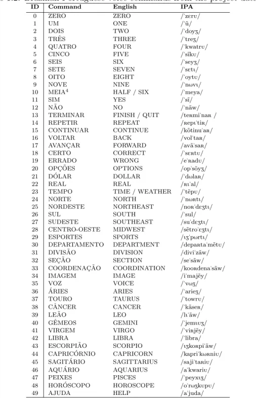
The adopted database for this project is the one constructed by Martins
[42]. It is constituted of 50 words, as presented in Table 1.2, three utterances
each, from 69 independent-speakers (46 men and 23 women, all adults). In
this work, we chose to represent Brazilian Portuguese words pronunciation
using the International Phonetic Alphabet (IPA). The IPA is an alphabetic
system of phonetic notation and it has been devised by the International
Phonetic Association as a standardized representation of all sounds in a given
spoken language2. By convention, we present the phonemic words between
slashes (/. . ./).
The captured audio signal for all the samples from this database had
passed through a hardware3 bandpass filter with cutoff frequencies (3dB)
of 300Hz and 3,400Hz. The audio signals were captured with a sampling
frequency of 8kHz and sample of 16 bits. For this work, all audio signals
from this database were converted to WAVEform Audio format (wav file extension), and has their respective length extended to support speech
seg-mentation testings. Also, they had white Gaussian noise added to each audio
file, to reach a Signal to Noise Ratio (SNR) of 30dB (considered a high level
SNR, i.e., a low level of noise compared to the signal).
2
For more information on IPA, please consult the “Handbook of the International Pho-netic Association: A Guide to the Use of the International PhoPho-netic Alphabet”, Cambridge University Press, 1999.
3
Table 1.2: Brazilian Portuguese voice commands from the project database.
ID Command English IPA
0 ZERO ZERO /"zErÚ/
1 UM ONE /"˜u/
2 DOIS TWO /"doyZ/
3 TRˆES THREE /"treZ/
4 QUATRO FOUR /"kwatrÚ/
5 CINCO FIVE /"s˜ıkÚ/
6 SEIS SIX /"seyZ/
7 SETE SEVEN /"sEtÌ/
8 OITO EIGHT /"oytÚ/
9 NOVE NINE /"nřvÌ/
10 MEIA4 HALF / SIX /"meya/
11 SIM YES /"s˜ı/
12 N ˜AO NO /"n˜aw/
13 TERMINAR FINISH / QUIT /teömi"naö/ 14 REPETIR REPEAT /öepÌ"tiö/ 15 CONTINUAR CONTINUE /k˜otinu"aö/
16 VOLTAR BACK /vol"taö/
17 AVANC¸ AR FORWARD /av˜a"saö/
18 CERTO CORRECT /"sEötÚ/
19 ERRADO WRONG /e"öadÚ/
20 OPC¸ ˜OES OPTIONS /op"s˜oyZ/ 21 D ´OLAR DOLLAR /"dřlaö/
22 REAL REAL /öÌ"al/
23 TEMPO TIME / WEATHER /"t˜epÚ/
24 NORTE NORTH /"nřötÌ/
25 NORDESTE NORTHEAST /noö"dEZtÌ/
26 SUL SOUTH /"sul/
27 SUDESTE SOUTHEAST /su"dEZtÌ/ 28 CENTRO-OESTE MIDWEST /s˜etro"EZtÌ/ 29 ESPORTES SPORTS /ÌZ"přrtÌ/ 30 DEPARTAMENTO DEPARTMENT /depaöta"m˜etÚ/ 31 DIVIS ˜AO DIVISION /divi"z˜aw/ 32 SEC¸ ˜AO SECTION /se"s˜aw/ 33 COORDENAC¸ ˜AO COORDINATION /kooödena"s˜aw/ 34 IMAGEM IMAGE /i"maj˜ey/
35 VOZ VOICE /"vřZ/
36 ARIES´ ARIES /"arieZ/
37 TOURO TAURUS /"towrÚ/
38 C ˆANCER CANCER /"k˜aseö/
39 LE ˜AO LEO /lÌ"˜aw/
40 GˆEMEOS GEMINI /"jemÌÚZ/ 41 VIRGEM VIRGO /"viöj˜ey/
42 LIBRA LIBRA /"libra/
43 ESCORPI ˜AO SCORPIO /ÌZkoöpi"˜aw/ 44 CAPRIC ´ORNIO CAPRICORN /kapri"křöniÚ/ 45 SAGIT ´ARIO SAGITTARIUS /saji"taöiÚ/ 46 AQU ´ARIO AQUARIUS /a"kwariÚ/
47 PEIXES PISCES /"peyxÌZ/
48 HOR ´OSCOPO HOROSCOPE /o"rřZkÚpÚ/
49 AJUDA HELP /a"juda/
4
Chapter 2
State of Art
The history on Speech Recognition systems goes back to 1950’s, when
we can detach the work of Davis, Biddulph and Balashek [15] published in
1952. There, they have state “the recognizer discussed will automatically
recognize telephone-quality digits spoken at normal speech rates by a single
individual, with an accuracy varying between 97 and 99 percent” . Inside a
low noise level controlled environment with a single speaker, they achieved
an excellent recognition rate for “0” to “9” spoken digits.
From 1950’s until now, several approaches have been discussed, mainly
divided into three essential stages: speech segmentation, features extraction,
and recognizer system. Besides the fact there are several intrinsic differences
between several types of speech recognition systems, inspiring Zue et al. [75]
to suggest parameters to label them (see Table 1.1), those three stages are
essential to all of them. The following chapter intends to explore some of the
widely used approaches to those stages.
2.1
Speech Segmentation
Speech segmentation could be defined as the boundary identification for
words, syllables, or phonemes inside captured speech signals. As stated by
Vidal and Marzal [69], “Automatic Segmentation of speech signals was
con-sidered both a prerequisite and a fairly easy task in most rather na¨ıve, early
research works on Automatic Speech Recognition”. Actually, speech
seg-mentation proved itself to be a complex task, specially when one is trying
to segment speech as we segment letters from a printed text. Several
al-gorithms were developed for the last decades. In the following paragraphs,
some widely used segmentation speech, as some developed by recent works
in the area, are presented.
The here namedClassical method uses energy and zero-crossing rate com-putations [56], in order to detect the beginning and the ending of a spoken
word inside a given audio signal. It is widely used until today, because it is
relatively simple to implement.
Another method, proposed by Mermelstein [45], uses a convex-hull
algo-rithm, to perform a “syllabification” of a spoken word inside a continuous
speech approach, i.e., the segmentation of the speech syllable by syllable.
Using an empirically determined loudness function, his algorithm “locates a
boundary within the consonant roughly at the point of minimal first-formant
frequency”. According to Mermelstein, “[...] the syllabification resulting
from use of the algorithm is generally consistent with our phonetic
expecta-tions”.
Bottom-up method, also known as Hybrid Endpoint Detector, was pro-posed by Lamel, Rabiner, et al [35], based on concepts of adaptive level
equalization, energy pulse detection and ordering of endpoints. They have
strat-2.1 Speech Segmentation 8
egy for finding endpoints using a three-pass approach in which energy pulses
were located, edited, and the endpoint pairs scored in order of most likely
candidates”.
Zhou and Ji [73] have designed a real-time endpoint detection algorithm
combining time-frequency domain. Their algorithm uses “the frequency
spec-trum entropy and the Short-term Energy Zero Value as the decision-making
parameters”. The presented results are not significant to enable comparisons.
Using regression fusion of boundary predictions, Mporas, Ganchev, and
Fakotakis [47] have studied “the appropriateness of a number of linear and
non-linear regression methods, employed on the task of speech segmentation,
for combining multiple phonetic boundary predictions which are obtained
through various segmentation engines”. They were worried about the
ex-traction of phonetic aligned in time, considered a difficult task. In their
work, they have employed 112 speech segmentation engines based on hidden
Markov models.
Some other works related to this subject could be found in the literature,
as the work of Liu et al. [36], regarding the automatic boundary detection
for sentences and disfluencies; the work of Yi and Yingle [71], that uses
the measure of the stochastic part of a complexity movement to develop
a robust speech endpoint detection in noisy environments; and the work
of Ghaemmaghami et al. [20], with a method that utilizes gradient based
edge detection algorithms, original from image processing field, to peform
2.2
Feature Extraction
It is very important for any speech recognition system design to select the
best parametric representation of acoustic data. This parametric
represen-tation is constituted of the features to be extracted from the speech signal.
Some parametric representation starts from the study of how the speech is
produced by human sound production system. Others starts from study of
how the speech is perceived by human auditory system.
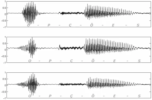
Figure 2.1 shows three different utterances from the same speaker for the
word OPC¸ ˜OES /op"s˜oyZ/. As one can see, those speech signals are more
distinguishable between each other than we expect them to be. The right
choice for the parametric representation is essential to minimize differences
between several utterances of the same phoneme.
2.2 Feature Extraction 10
2.2.1
Human Sound Production System Based Models
Linear predictive coding
Linear prediction theory can be traced back to the 1941 work of
Kol-mogorov1 referenced in Vaidyanathan [68]. In this work, Kolmogorov
consid-ered the problem of extrapolation of discrete time random processes. From
the first works that explored the application in speech coding, we can dettach
the work of Atal and Schroeder [3] and that of Itakura and Saito2
referen-ced in Vaidyanathan [68]. Atal and Itakura independently formulated the
fundamental concepts of Linear Predictive Coding (LPC).
Itakura [27], Rabiner and Levinson [54], and others, have started the
proposition of using LPC with pattern recognition technologies to enable
speech recognition applications. LPC represents the spectral envelope of a
speech digital signal, using the information of a linear predictive model. LPC
is actually a close approximation of a speech production system: the speech
is produced by a buzzer (glottis), characterized by loudness and pitch, at the
end of a tube (vocal tract), characterized by its resonance, with occasional
hissing and popping sounds (made by tongue, lips and throat).
LPC is widely used in speech analysis and synthesis. Some recent
exam-ples of speech recognition systems that uses LPC could be the work of Thiang
[66], that uses LPC to extract word data from a speech signal in order to
control the movement of a mobile robot, and the work of Paul [51], that
presents the Bangla speech recognition system which uses LPC and cepstral
coefficients to construct the codebook for the artificial neural network.
1
Kolmogorov, A. N. Interpolation and extrapolation of stationary random sequences,
Izv. Akad. Nauk SSSR Ser. Mat. 5, pp. 3–14, 1941.
2
Cepstrum
The term cepstrum was first coined by Bogert et al.3, referenced in Op-penheim and Schafer [48], and they mean “the spectrum of the log of the
spectrum of a time waveform”. The spectrum of the log spectrum shows a
peak when the original time waveform contains an echo. This new spectral
representation domain is not the frequency nor the time domain. Bogert et
al. chose to refer to it as the quefrency domain.
The cepstrum could be very important to many speech recognition
sys-tems. As stated by Oppenheim and Schafer [48], “[...] the cepstral
coeffi-cients have been found empirically to be a more robust, reliable feature set
for speech recognition and speaker identification than linear predictive
cod-ing (LPC) coefficients or other equivalent parameter sets”. There are a vast
family of cepstrum, several of them applied with success to speech
recogni-tion systems, like linear predicrecogni-tion cepstrum [70], shifted delta cepstrum4 [8],
and mel-frequency cepstrum [16].
An example on using cepstrum to speech recognition could be found in
the work of Kim and Rose [32] that proposes a cepstrum-domain model
combination method for automatic speech recognition in noisy environments.
As a recent example, we can dettach the work of Zhang et al. [72] that uses
time-frequency cepstrum, based on a horizontal discrete cosine transform of
the cepstrum matrix for de-correlation, and performs a heteroscedastic linear
discriminant analysis to achieve a novel algorithm to language recognition
field.
3
B.P. Bogert, M.J.R. Healy, and J.W. Tukey, “The quefrency alanysis of time series for echoes: Cepstrum, pseudo-autocovariance, cross-cepstrum, and saphe cracking, in Time Series Analysis, M. Rosenblatt, Ed., 1963, ch.15, pp. 209243.
4
2.2 Feature Extraction 12
2.2.2
Human Auditory System Based Models
Inside feature extraction theme, the human auditory system model is
dis-cussed for over a hundred years. Actually, the search for a reliable auditory
filter to extract the best parametric representation of acoustic data is the
main quest for several researchers worldwide. The auditory filters, according
to Lyon et al. [38], “include both those motivated by psychoacoustic
experi-ments, such as detection of tones in noise maskers, as well as those motivated
by reproducing the observed mechanical response of the basilar membrane or
neural response of the auditory nerve”. They have also stated that “today,
we are able to represent a wide range of linear and nonlinear aspects of the
psychophysics and physiology of hearing with a rather simple and elegant set
of circuits or computations that have a clear connection to underlying
hy-drodynamics and with parameters calibrated to human performance data”.
In this section, we present some of those human auditory system models
that enables the extraction of different features from the speech signals.
Mel-frequency Cepstrum
From the family of cepstrum, the Mel-frequency Cepstrum is widely
used for the excellent recognition performance they can provide [16].
Mel-frequency cepstrum (MFC) is a representation of the short-term power
spec-trum of a sound, based on a linear cosine transform of a log power specspec-trum
on a nonlinear mel scale of frequency. The mel scale (comes from “melody”
scale), proposed by Stevens et al. [64], is based on pitch comparisons from
listeners, i.e., mel scale is a perceptual scale of pitches that were judged equal
is widely referenced when exploring Mel-frequency Cepstrum history, but
Mermelstein usually credits John Bridle’s work5 for the idea.
According to Combrinck [9], “from a perceptual point of view, the
mel-scaled cepstrum takes into account the non-linear nature of pitch perception
(the mel scale) as well as loudness perception (the log operation). It also
models critical bandwidth as far as differential pitch sensitivity is concerned
(the mel scale)”. Widely used in speech recognition systems, we can found
a recent example in the work of Bai and Zhang [4], where they extract
lin-ear predictive mel cepstrum features through “the integration of Mel
fre-quency and linear predictive cepstrum”. Another recent example, the work
of Kurian and Balakrishnan [34], extracts MFC coefficients to implement a
speech recognition system for the recognition of Malayalam numbers.
Gammatone Filterbank
Aertsen and Johannesma [2] had introduced the concept of gammatone,
“an approximative formal description of a single sound element from the
vocalizations [...]”. According to Patterson [50], the response of a gammatone
filter “transduces” the basilar membrane motion, converting it into a
multi-channel representation of “[...] the pattern of neural activity that flows from
the cochlea up the auditory nerve to the cochlear nucleus”. In other words,
Patterson6, referenced in [63], states that “Gammatone filters are derived
from psychophysical and physiological observations of the auditory periphery
and this filterbank is a standard model of cochlear filtering”.
5
J. S. Bridle and M. D. Brown, “An experimental automatic word recognition system,” Tech. Rep. JSRU Report No. 1003, Joint Speech Research Unit, Ruislip, England, 1974.
6
R. D. Patterson,et al., “Auditory models as preprocessors for speech recognition,” in
2.2 Feature Extraction 14
A gammatone filterbank is composed of as many filters as the desired
number of output channels. Each channel is designed to have a center
fre-quency and a respective equivalent rectangular bandwidth (ERB). The filter
center frequencies are distributed across frequency in proportion to their
bandwidth. Greenwood had come with the assumption that critical
band-width represent equal distances on the basilar membrane and also had defined
a frequency-position function [22]. Glasberg and Moore [21] have summarized
human data on the ERB for an auditory filter.
The preference of using gammatone filters to simulate the cochlea is
sensed by Schluter et al. [60], “the gammatone filter (GTF) has been hugely
popular, mostly due to its simple description in the time domain as a
gamma-distribution envelope times a tone”. Recent examples of using GTF includes
the works of Shao and Wang [63], and Shao et al. [62], that respectively
pro-poses and applies the gammatone frequency cepstrum, based on the discrete
cosine transform applied to features extracted from the gammatone filter
res-ponse to speech signal. Another example is the work of Schluter et al. [60]
that presents “an acoustic feature extraction based on an auditory filterbank
realized by Gammatone filters”.
Wavelet filterbank
The name wavelet was firstly coined by Morlet et al.7. The wavelet
trans-form is described by Daubechies [14] as “a tool that cuts up data or functions
or operators into different frequency components, and then studies each
com-ponent with a resolution matched to its scale”. Daubechies also made the
correspondence between the human auditory system and the wavelet
trans-form, at least when analyzing the basilar membrane response to the pressure
7
amplitude oscillations transmitted from the eardrum. According to her, “the
occurrence of the wavelet transform in the first stage of our own biological
acoustical analysis suggests that wavelet-based methods for acoustical
anal-ysis have a better chance than other methods to lead, e.g., to compression
schemes undetectable by our ear”.
The work of Gandhiraj and Sathidevi [19] proposes a cochlea model based
on a high resolution Wavelet-Packet filterbank. The latest published works
from this research [52, 53] have used Wavelet-Packet filterbank to extract
features from the speech signals. Another example of recent works using
wavelets for speech recognition is the work of Maorui et al. [40], that uses
the wavelet packet transform to evaluate what they present as the improved
mel-frequency cepstral coefficients.
Two Filter Cascades
As stated by Lyon et al. [38], the polezero filter cascade (PZFC) “has
a much more realistic response in both time and frequency domains, due to
its closer similarity to the underlying wave mechanics, and is not much more
complicated”. Since [37], Lyon has stated that “the filter-cascade structure
for an cochlea model inherits two key advantages from its neuromorphic
roots: efficiency of implementation, and potential realism”.
We have not found recent works that use this approach as the parametric
representation of speech, but we realize that PZFC is worth to be
2.3 Speech Recognition 16
2.3
Speech Recognition
Speech recognition is considered a pattern recognition problem, where
each kind of phoneme, spoken word, emotion, or even the individual identity
of a given set of speakers constitutes a different class to try fitting my testing
pattern. This pattern is constituted by the features which are extracted
from each speech signal analyzed by the recognizer system. A successful
recognition means the recognizer system successfully indicates the expected
class of a given input speech signal. Some of the most widely used recognizers
are presented in the following. As convention, training set identifies the set
of patterns presented to the recognizer in the learning stage; testing set
identifies the set of patterns, or an individual pattern, that the recognizer
must make an inference about which class it belongs, after the learning stage.
Clustering Algorithms
From all various techniques that can be considered a clustering algorithm,
we shall consider one elementary, named K-means clustering. We start with the evaluation of each predetermined class mean, i.e., the mean of all
n-dimensional pattern vector obtained by the feature extraction stage for all
speech signals that we know from that specific class. Those means are known
as class centroids. K-means clustering algorithm will check for each pattern
vector of the testing set which centroid is the one most closer to it. This
mea-surement of distance can vary from an implementation to another. Common
used distance measurements include the widely known Euclidean distance,
Mahalanobis distance8, or even Itakura-Saito distance [27].
8
Support Vector Machine
Cortes and Vapnik [11] have proposed the Support-vector Networks, later
named as Support Vector Machines (SVM). They have presented SVM as “a
new learning machine for two-group classification problems”. Basically, SVM
relies on the preprocessing of the data to represent patterns in a much high
dimension. The main idea is that when applying an appropriate nonlinear
mapping function in order to augment the original feature space to a
suffi-ciently high dimension, data from two categories can always be separated by
a hyperplane.
From the recent works mentioned before, the works [4, 72] uses SVM as
the speech recognition system. For more information about SVM, we suggest
the work of Burges [7].
Artificial Neural Networks
According to Fausett [17], an Artificial Neural Network (ANN) is “an
information-processing system that has certain performance characteristics
in common with biological neural networks”. The motivation of studying
ANNs is their similarity to successfully working biological systems, which
consist of very simple but numerous nerve cells (neurons) that work
mas-sively parallel and have the capability to learn from training examples [33].
The main consequence of this learning ability of ANNs is that they are able
of generalizing and associating data, i.e., ANN can make correct inferences
about data that were not included in the training examples.
The first attempt to simulate a biological neuron was performed in 1943
by McCulloch and Pitts [43]. Since then, several neuron approaches and
architectures have been developed increasing this way the family of artificial
2.3 Speech Recognition 18
recognition is the Multilayer Perceptron (MLP), or multilayer feed-forward
networks [59], based on Rosenblatt’s Perceptron neuron model [58].
Note that the universal approximation theorem from mathematics, also
known as the Cybenko theorem, claims that the standard multilayer
feed-forward networks with a single hidden layer that contains finite number of
hidden neurons, and with arbitrary activation function, are universal
approx-imators on a compact subset of ℜn [12]. This theorem was first proved by Cybenko[13] for a sigmoid activation function. Hornik [25] concludes that “it
is not the specific choice of the activation function, but rather themultilayer feedforward architecture itself which gives neural networks the potential of being universal learning machines” [emphasis in original].
From the recent works mentioned before, the works [19, 51, 52, 53, 40]
use ANN architectures as the speech recognition system. For more
infor-mation about ANN, we suggest the works of Fausett [17], Haykin [23], and
Kriesel [33].
Hidden Markov Models
The Hidden Markov Model (HMM) can be defined as afinite set of states, each of which is associated with a probability distribution, multidimensional
in general. There are a set of probabilities called transition probabilities that rules over the transitions among the states. According to the associated
probability distribution, a particular state can generate one of the possible
outcomes. The system being modeled by a HMM is assumed to be a Markov
process with unobserved (or hiddden) states. A Markov process is defined by
a sequence of possibly dependent random variables with the property that
last state. In other words, the future value of such a variable is independent
of its past history.
From the recent works mentioned before, the works [32, 66, 34] use HMM
as the speech recognition system. For more information about HMM, we
suggest the work of Rabiner [55].
Hybrid HMM/ANN
Hybrid HMM/ANN systems combine artificial neural networks (ANN)
and hidden Markov models (HMM) to perform dynamic pattern recognition
tasks. In the speech recognition field, hybrid HMM/ANN can lead to very
powerful and efficient systems, due to the combination of the discriminative
ANN capabilities and the superior dynamic time warping HMM abilities
[57]. One of the most popular hybrid approach is described by Hochberg et
al. [24]. Rigoll and Neukirchen [57] have presented a new approach to hybrid
HMM/ANN which performs, as stated by them, “already as well or slightly
better as the best conventional HMM systems with continuous parameters,
and is still perfectible”.
The hybrid HMM/ANN systems are a modified form of an earlier design
known as “discriminant HMMs” which was initially developed to directly
es-timate and train ANN parameters to optimize global posterior probabilities.
In hybrid HMM/ANN systems, all emission probabilities can be estimated
to the ANN outputs and those probabilities are referred to as conditional
transition probabilities [6].
Recent works using HMM/ANN hybrid models include the work of [31],
which proposes a novel enhanced phone posteriors to improve speech
recog-nition systems performance (including HMM/ANN), and the work of Bo et
2.4 Choices for this Work 20
existing speech access control system. Another example, the work of Huda et
al. [26], based on the extraction of distinctive phonetic features, proposes the
use of two ANN stages with different purposes before reaching a HMM-based
classifier.
For more information about hybrid HMM/ANN, we suggest the work of
Bourlard and Morgan [6].
2.4
Choices for this Work
From earlier conducted tests based on this project database, we have
cho-sen Mel-frequency Cepstrum as the parametric representation of our acoustic data. Because of its simple implementation and great ability of
generaliza-tion, we have chosen an Artificial Neural Network architecture, theMultilayer Perceptron, as the recognizer system for this project. Details on those can be found in Chapter 3.
For the purposes of this work, we have chosen Classical and Bottom-up
methods to compare performances with this project proposed word boundary
detector based on the Teager energy operator. The proposed word boundary
detector method and the comparisons with those other methods can be found
Theoretical Background
The results derived from this work may support the implementation of
speech recognition systems described by the parameters shown in Table 3.1.
Those parameters are based on the ones proposed by Zue, Cole and Ward [75].
Table 3.1: Proposed speech recognition system
Parameters Range
Speaking Mode Isolated words Speaking Style Spontaneous speech
Enrollment Speaker-independent
Vocabulary 50 words
Language Model Finite-state
SNR High (≈ 30dB)
Transducer Electret condenser microphone
Regarding high Signal to Noise Ratio (SNR) here stated, the system
des-cribed in this work could also act in lower SNR environments, but some
configuration adjustments are required in the speech segmentation stage
des-cribed in Chapter 4.
3.1 Audio Signal Capture 22
The recognition system described in the present work is build with widely
used steps, but the simpler ones. Besides speech segmentation, fully
devel-oped inside this research, all other stages could be found in related literature.
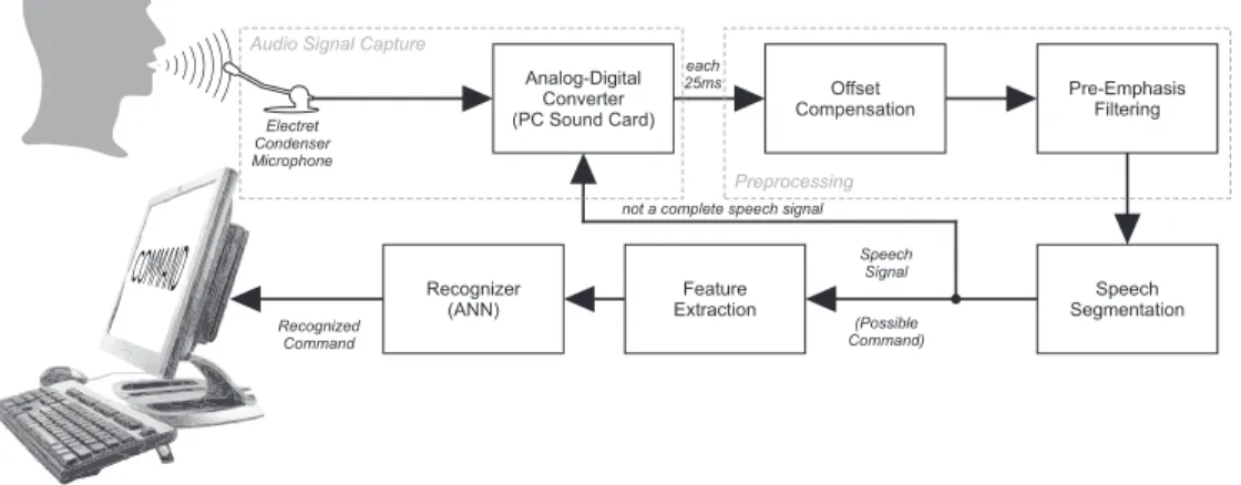
The proposed system block diagram for this research project is presented in
figure 3.1. Each block is explained throughout this chapter.
Feature Extraction Recognizer (ANN) Analog-Digital Converter (PC Sound Card)
Speech Segmentation Offset Compensation Pre-Emphasis Filtering each 25ms Preprocessing Electret Condenser Microphone (Possible Command) Recognized Command Speech Signal not a complete speech signal
Audio Signal Capture
Figure 3.1: Proposed speech recognition system block diagram.
3.1
Audio Signal Capture
By using a electret condenser microphone, the audio signal is captured
using the sampling frequency of 8kHz and the word-length of 16 bits. As
stated by Nyquist-Shannon sampling theorem[61], “if a functionf(t) contains
no frequencies higher than W cps1, it is completely determined by giving its
ordinates at a series of points spaced 1
2W seconds apart”. So, capturing an
audio signal with a sampling frequency of 8kHz, one can ensure the reliable
capture of only 0 to 4kHz frequency components from the given signal.
1
The specifics of the analog-to-digital conversion are not part of the present
dissertation. Applications which will be developed in this research will use
the analog-to-digital converter featured in most PC sound cards.
Meanwhile, for this work, a database of prerecorded audio files (see
Sec-tion 1.3) was used to evaluate the potentialities of the system. For the
conducted tests shown in this work, the loaded recorded audio files were
constituted by values inside the [-1,1] interval.
3.2
Preprocessing
European Telecommunications Standards Institute has published the ES
201 108 V1.1.3[1] standard2 to guide transmissions over mobile channels.
ETSI Standards are respected over all in Europe, including Portugal, which
ensures ETSI concerns about Portuguese language among others. ES 201
108 standard has significant information on preprocessing for speech signals.
3.2.1
Offset compensation
After analog-to-digital conversion, a notch filtering operation is applied
to the digital samples of the input audio signal to remove their DC offset,
producing a offset-free input signal. This operation is also known as
ze-ropadding. The notch filtering operation is done as presented in equation
(3.1), the same as in item (4.2.3) from ES 201 108 standard [1]:
sof(n) =sin(n)−sin(n−1) + 0.999·sof(n−1), (3.1)
2
3.3 Speech Segmentation 24
where sof is the offset-free input signal; sin is the input signal; and n is the
sample index. It assumes, for n = 0, that sof(0) =sin(0).
3.2.2
Pre-emphasis filtering
Before any other computation, the offset-free audio signal is then
pro-cessed by a simple pre-emphasis filter. After pre-emphasis filtering, the
ave-rage speech spectrum turns to roughly flat.
The application of the pre-emphasis filter to the offset-free input signal
is done by applying Equation (3.2), the same as in item 4.2.6 from ES 201
108 standard:
spe(n) = sof(n)−0.97·sof(n−1), (3.2)
wherespe is the pre-emphasis filtered input signal;sof is the offset-free input
signal; and nis the sample index. It assumes, forn= 0, thatspe(0) =sof(0).
3.3
Speech Segmentation
The spoken word segmentation algorithm pretends to detect the starting
and the ending points of a speech waveform within a sampled audio waveform
signal. This process is known as boundary detection of the speech, detection
of the speech endpoints, speech segmentation, or spoken word isolation.
A novel method for speech segmentation, based on the Teager Energy
Operator (TEO), was developed during this research. This method is detailed
in Chapter 4, named as “TEO-based method for Spoken Word Segmentation”
(TSWS). The result of this stage is a word-like speech signal segmented from
3.3.1
The Teager Energy Operator
In the work of Teager and Teager3 on nonlinear modeling of speech,
re-ferenced in Maragos et al. [41], an energy operator on speech-related signals
is first presented.
In his work, Kaiser has discussed the properties of that Teager’s
energy-related algorithm — later designed as the Teager Energy Operator (TEO),
or the Teager-Kaiser Operator — which, “by operating on-the-fly on signals
composed of a single time-varying frequency, is able to extract a measure of
the energy of the mechanical process that generated this signal” [29].
When the signal consists of several different frequency components — like
in captured speech signals — Kaiser states that, to use this energy operator
effectively, “it is important to pass the signal through a bank of bandpass
filters first; the algorithm is then applied to the outputs from each of these
bandpass filters” [29].
Kaiser [30] has also defined both TEO in the continuous and discrete
domains as “very useful ’tools’ for analyzing single component signals from
an energy point-of-view” [emphasis in original].
TEO is then defined by Equation (3.3), in the continuous domain, and
by Equation (3.4), in the discrete domain [30]. Note that, in the discrete
domain, this algorithm uses only three arithmetic operators applied to three
adjacent samples of the signal for each time shift.
Ψ [x(t)],
(
dx(t) dt
)2
−x(t)· d
2x(t)
dt2 , (3.3)
where Ψ is the TEO operator; and x(t) is the amplitude of the signal at the
time t.
3
3.4 Feature Extraction 26
Ψ [x(n)] =x2n−xn−1·xn+1, (3.4)
where Ψ is the TEO operator; and x(n) is the nth sample of the discrete
signal.
Another aspect of TEO, observed when it is applied to speech signals
without a bandpass filterbank previous stage, is interesting for this research:
when one applies TEO to signals composed of two or more frequency
compo-nents — a speech signal, for example — TEO does not give the energy of the
system generating this composite signal, but, according to Kaiser [29], “it is
as if the algorithm is able to extract the envelope function of the signal”.
3.4
Feature Extraction
According to Martins [42], to evaluate the features (or coefficients) to be
extracted from the input speech signals, it is usual to divide those signal into
non-overlapping frames. Each of those frames has to be multiplied with a
Hamming window, presented in equation (3.5), in order to keep the continuity
of the first and the last points in the frame [16], [1]. To ensure an overlapping
relation between windows and frames, each window size must be greater than
the frame size, as shown in Figure 3.2.
h(n) =
0.54−0.46·cos(2πn
N−1 )
, if 0 ≤n≤N −1
0, otherwise , (3.5)
where h(n) is the window resultant of nth sample of the frame; and N is the
total number of samples from each frame.
Martins has also designed a method to keep the same numbers of
frame 1 frame 2 frame 3 frame 4 window 1 window 3
window 2 window 4
Figure 3.2: Overlapping of windows on frames for coefficient evaluation.
signal is divided into a fixed number of 80 frames. A window of 20ms 4 is
then chosen to run through the frames. If the evaluated frame size is greater
than the window size, turning the window overlap impossible, the window
size is then adjusted to 1.5 times the frame size. The algorithm for setting
frame and windows sizes, evaluated in number of samples, is presented in
Algorithm 3.1.
Algorithm 3.1 Setting frame and window sizes. f r ← length(signal)/80 // frame size (f r)
wd←0.02∗F s // sampling frequency (F s), window size (wd)
if f r > wd then
wd= 1.5∗f r
end if
Different timbres in speech signals correspond to different energy
distri-bution over frequencies, as can be shown by a spectral analysis. Therefore,
the Fast Fourier Transform (FFT) is performed to obtain the magnitude
frequency response of each “windowed” frame.
After, the magnitude frequency response obtained by FFT is multiplied
by a set of 16 triangular bandpass filters, in order to get the log-energy
of each filter respective output. The center frequencies of those filters are
equally spaced along the Mel frequency scale. The Mel scale (comes from
“melody” scale), proposed by Stevens, Volkman and Newman[64], is based on
pitch comparisons from listeners, i.e., Mel scale is a perceptual scale of pitches
that were judged equal in distance from one another by tested listeners. The
4
3.4 Feature Extraction 28
relation from Hertz to Mels is achieved by the equation (3.6), as presented
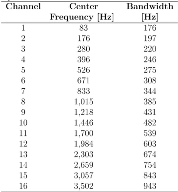
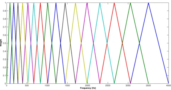
by O’Shaughnessy [49]. The relation plot is shown in Figure 3.3. Table 3.2
and Figure 3.4 presents the center frequencies and the bandwidth of each of
the 16 triangular bandpass filters.
m = 2595·log10
(
1 + f 700
)
, (3.6)
where m is the frequency in Mels; and f is the frequency in Hz.
Figure 3.3: Hertz scale versus Mel scale.
Finally, Mel-frequency Cepstral Coefficients (MFCC) could be extracted
from the input speech signal. The choice of using MFCC as features to be
extracted from speech signals comes from the widely use of those coefficients
and the excellent recognition performance they can provide [16, 42]. MFCC,
generalized from the ones computed by Davis and Mermelstein [16], is
Table 3.2: Center frequencies and respective bandwidth for the designed 16 triangular bandpass filters.
Channel Center Bandwidth
Frequency [Hz] [Hz]
1 83 176
2 176 197
3 280 220
4 396 246
5 526 275
6 671 308
7 833 344
8 1,015 385
9 1,218 431
10 1,446 482
11 1,700 539
12 1,984 603
13 2,303 674
14 2,659 754
15 3,057 843
16 3,502 943
MFCCi = N
∑
k=1
Xk·cos
[
i
(
k− 1 2
)
π N
]
, i= 1,2, . . . , M, (3.7)
whereM is the number of cepstral coefficients;N is the number of triangular
bandpass filters; and Xk represents the log-energy output of the kth filter.
The set of MFCC constitutes the Mel-frequency Cepstrum (MFC), which
is derived from a type of cepstral representation of the audio signal. The
main difference from a normal cepstrum5 is that MFC uses frequency bands
equally spaced on the Mel scale (an approximation to the response of human
auditory system) and normal cepstrum uses linearly-spaced frequency bands.
5
3.5 The Recognizer 30
Figure 3.4: Filters for generating Mel-Frequency Cepstrum Coefficients.
For a given input speech signal, we start dividing it into 80 frames and,
for each frame, we end up evaluating 16 MFCC. Concatenating all those
coefficients in a row, we get 1,280 coefficients (the feature vector) to act as
the input vector for the recognizer system.
3.5
The Recognizer
The option for using an artificial neural network (ANN) model to act as
the recognition system is just an aspect of this work. As stated before, an
artificial neural network is defined by Fausett as “an information-processing system that has certain performance characteristics in common with
bio-logical neural networks” [17]. Fausett also characterizes an ANN by its
ar-chitecture, its activation function, and its training (or learning) algorithm.
The breadth of ANN’s applicability is suggested by the areas in which they
are currently being applied: signal processing, control, pattern recognition,
ANNs are being applied with great success rates [65]. However, some
hy-brid model solutions, as the ones which combine ANN with hidden Markov
models (HMMs), have shown better results for speech recognition systems
[5, 26, 31].
Feature Extraction
Pattern Recognized Dataset
x0
x1
x2
xI
y0
y1
yJ h0
h1
hK-1
hK h2
I Kmatrix of synaptic weights
× K Jmatrix
of synaptic weights ×
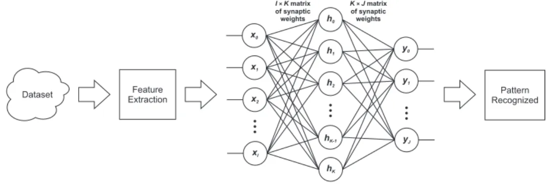
Figure 3.5: Diagram with a I×K×J MLP acting as recognizer.
Multi-layer Perceptron (MLP) is an ANN architecture relatively simple
to implement. It is very robust when recognizing different patterns from
the ones used for training, and it has wide spread use to handle pattern
recognition problems. Based on Rosenblatt’s Perceptron neuron model [58],
it typically uses an approach based on the Widrow-Hoff backpropagation
of the error [17] as the supervised learning method. Figure 3.5 presents
the diagram of a general MLP with I input units, K hidden units, and J
output units. Note that the number of input units from a MLP is the same
number of coefficients generated after the feature extraction stage. Likewise,
the number of output units is generally the number of existing classes for
pattern classification (or recognition).
The desire of effectively recognize isolated spoken words can be classified
3.5 The Recognizer 32
of robustness and simplicity of implementation, a single hidden layer MLP6
is the chosen ANN architecture for this project recognizer.
in1
out in2
in3
inN
y= ( )f x
-5 -4 -3 -2 -1 0 1 2 3 4 5 -1 -0.8 -0.6 -0.4 -0.2 0 0.2 0.4 0.6 0.8 1 f(x)=tanh(x) x w1 b
w inn∙ n
Σ
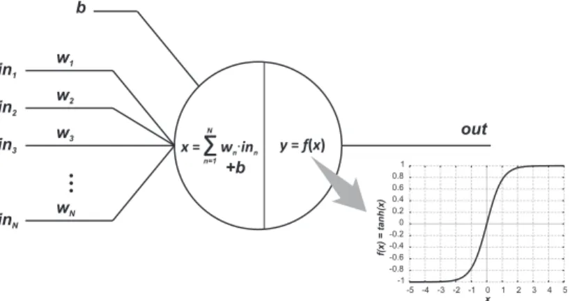
n=1 N x= +b w2 w3 wNFigure 3.6: A Perceptron with the hyperbolic tangent as the activation func-tion.
Each neuron of the chosen MLP, presented in Figure 3.6, has the
hyper-bolic tangent (tanh) as the activation function. Neurons work as mathemat-ical functors, using as argument the weighted arithmetic mean from input
values, weighted by their respective synaptic weights (wi) plus a bias (b).
The output of a neuron is the result of applying the activation function in
that weighted mean argument. The neuron used in the ANN architecture
could be described by equation (3.8). Activation of a neuron means that
the result of that neuron’s function (output level) is above a predetermined
threshold.
Om = tanh
(
bm+ N
∑
n=1
wn,m ·In
)
, (3.8)
where Om is the expected output of the mth neuron; bm is the bias value for
the mth neuron;w
n,m is the synaptic weight of themth neuron correspondent
6
to nth input; N is the total number of inputs; and I
n is the nth input of the
neuron.
The concept of training an ANN means iterative updates of the ANN’s
synaptic weights and biases. Supervised training means the training
algo-rithm takes into account the difference of the expected output vector (or
target vector) and the actual output vector generated when ANN is exposed
to a single input vector. This accounting is part of the correction term
cal-culation for the synaptic weights updates. The training process is repeated
until the ANN reaches an acceptable total error of performance, or it achieves
a maximum number of training epochs.
Different types of algorithms were verified to enable a fast training for the
recognizer. Scaled Conjugate Gradient [46] was then chosen as the supervised training algorithm and Bayesian Regularization algorithm7 [67] was chosen to enable ANN’s performance evaluation during the training.
The project recognizer is then implemented as a single hidden layer MLP
with 1,280 input units, 100 hidden units and 50 output neurons. Each
out-put neuron corresponds to a different voice command and its activation is
equivalent to the recognition of its respective command (see Table 1.2 for the
group of voice commands to be recognized). The project MLP uses real
num-bers as input vectors (input ∈ ℜ) and bipolar target output vectors (target output could be -1 or 1).
3.5.1
Confusion Matrices
Confusion matrix (CM), or table of confusion, is a visualization tool
typ-ically used in supervised learning pattern recognition systems. Each row of
the matrix represents the actual output class recognized by the system, while
7
3.5 The Recognizer 34
each column represents the correct target class the system should recognize.
Confusion matrices enable an easy visualization of the system mislabels, i.e.,
Proposed Method for Speech
Segmentation
As stated by Lamier, Rabiner, et al [35], “accurate location of the
end-points of an isolated word is important for reliable and robust word
recogni-tion”. Due to its importance, we had searched for a reliable and robust speech
segmentation method. Finally, during this research, we have developed a
novel method for speech segmentation, based on the Teager Energy
Opera-tor (TEO), also known as the Teager-Kaiser OperaOpera-tor. The proposed method
was named “TEO-based method for Spoken Word Segmentation” (TSWS).
The TSWS method has evolved from the premise that TEO can emphasize
speech regions from an audio signal, as presented in other works [53].
The following chapter presents TSWS as a method for speech
segmenta-tion, the results achieved when applying it to an American English support
database, and comparisons with Classical [56] and Bottom-up [35] speech