FACULTY OF ELECTRICAL ENGINEERING
UNIVERSITY OF BANJA LUKA
VOLUME 3, NUMBER 2, DECEMBER 2009
1
Phone: +387 51 211824 Fax: +387 51 211408
E L E C T R O N I C S
Web: www.electronics.etfbl.net E-mail: [email protected]
Editor-in-Chief:
Branko L. Doki , Ph. D.
Faculty of Electrical Engineering
University of Banja Luka, Bosnia and Herzegovina E-mail: [email protected]
International Editorial Board:
• Goce Arsov, St. Cyril and Methodius University, Skopje, Republic of Macedonia
• Petar Biljanovi , University of Zagreb, Croatia
• Milorad Boži , University of Banja Luka, Bosnia and Herzegovina
• emal Koloni , University of Banja Luka, Bosnia and Herzegovina
• Vladimir Kati , University of Novi Sad, Serbia
• Van o Litovski, University of Niš, Serbia
• Danilo Mandi , Imperial College, London, United Kingdom
• Vojin Oklobdžija, University of Texas at Austin, USA
• Zorica Panti , Wentworth Institute of Technology, Boston, USA
• Aleksandra Smiljani , University of Belgrade, Serbia
• Slobodan Vukosavi , University of Belgrade, Serbia
• Volker Zerbe, Technical University of Ilmenau, Germany
• Mark Zwoli ski, University of Southampton, United Kingdom
• Deška Markova, Technical University of Gabrovo
Secretary:
Petar Mati , .Sc. E-mail: [email protected] Mladen Kneži ,
E-mail: [email protected] Željko Ivanovi ,
E-mail: [email protected]
Publisher:
Faculty of Electrical Engineering
University of Banja Luka, Bosnia and Herzegovina
Address: Patre 5, 78000 Banja Luka, Bosnia and Herzegovina Phone: + 387 51 211824
Fax: + 387 51 211408 Web: www.etfbl.net
YMPOSIUMINFOTEH®-JAHORINA is continuation of the International symposium JAHORINA that was held last time on April 1991. The main organizer of the Symposium is the Faculty of Electrical Engineering East Sarajevo and the co-organizer is the Faculty of Electrical Engineering Banja Luka. The Symposium is supported by The Faculty of electrical engineering, Belgrade, Serbia, the Faculty of electronics, Niš, Serbia, the Faculty of technical sciences, Novi Sad, Serbia.
The goal of the Symposium is multidisciplinary survey of the actual state in the information technologies and their application in the industry plants control systems, the communication systems, the manufacturing technologies, power system, as well as in the other branches of interest for the successful development of our living environment.
During the first Symposium, that was held on 12-14 March 2001, 53 works have been presented, six companies presented their development and manufacturing programs in telecommunications, power electronics, power systems and process control systems. More than hundred participants took part in the Symposium working. Round table about potentials and possibilities of economic cooperation between Republic of Srpska and FR Yugoslavia has been held during the Symposium, regarding successful appearance at domestic and foreign market.
During the second Symposium, that was held on 25-27 March 2002, 76 works have been presented, and five companies presented their development and manufacturing programs. More than hundred and thirty participants took part in Symposium working. Round table entitled "Reforms in high education – step forward to the European University" has been held during the Symposium.
The third Symposium was held on 24-26 March 2003. More than hundred and fifty participants took part in the Symposium working. At the Symposium 73 papers have been presented and nine student papers. Four companies presented their development and manufacturing programs. Round table entitled "New Technologies and Industrial Production Capabilities for small Countries in the Transition Process" has been held during the Symposium.
The fourth Symposium was held on 23-25 March 2005. At the Symposium two invited papers, eighty and three papers and three student's papers have been presented. Three companies presented their development and manufacturing programs. All papers are presented in symposium proceedings, CD version (ISBN-99938-624-2-8).
The fifth Symposium was held in 2006, March 23 – 25. The Symposium was dedicated to the 150th anniversary of
Nikola Tesla’s birth. It was the first official manifestation in the Republic of Srpska dedicated to this jubilee. The university
character of this traditional international scientific and professional gathering was reflected in a complete and multidisciplinary approach to the discussion of themes within the discussion forums, lectured and presentations. There were exposed 137 papers which passed the review, and 172 guests of the symposium were registered.
The sixth Symposium was held in 2007, March 28 – 30. and it was dedicated to global warming and its side effects. The opening lecture by call was held by Ana Pavlovi , physicist of meteorology and living environment modeling from Faculty of Technical Sciences, University of Novi Sad. 160 papers were written for the Symposium, and 131 of them were accepted, including 6 students’ works.
The seventh Symposium was held in 2008, March 26 – 28. The Symposium was dedicated to the life and work of Milutin Milankovi , and Professor Mili Stoji , Ph. D. from the University of Belgrade had an extraordinary introductory lecture about the life and achievements of this great Serbian scientist. The Symposium was opened by the inspiring speech of the academician Rajko Kuzmanovi , the President of the Republic of Srpska. Over 220 papers were written for the Symposium, and 169 of them were accepted.
The eighth fourth Scientific – Professional Symposium INFOTEH®-JAHORINA 2009 was held on 18-20 March 2009 in the hotel Bistrica at Jahorina. The Symposium was dedicated to the year of astronomy. The opening lecture by call “The Origin and the Fate of the Universe” was held by Professor Pavle Kalu er i , Ph. D. from the Faculty of Electrical Engineering, University of East Sarajevo. The main topics of the Symposium were: Computer science application in control systems, Information-communication systems and technologies, Information system in manufacturing technologies, Information technologies in power systems, Information technologies in other branches of interest. Over 260 papers were written for the Symposium, and 199 of them were accepted and exposed, including 19 students’ works, and 265 guests of the symposium were registered.
I would like to invite all readers of the “Electronics” journal to take active participation at the next Symposium INFOTEH®-JAHORINA. Updated information can be obtained from the Symposium web page:
http://www.infoteh.rs.ba.
Professor emeritus Slobodan Milojkovi . Ph. D. Chairman of the Programming Commitee,
INFOTEH®-JAHORINA 2009
Guest Editorial
Abstract—The paper offers a possibility of upgrading
conventional PD controlled positional systems into high-precision tracking systems using active compensators. For improving of tracking as well as disturbance rejection capabilities of these systems, two digital active compensators are used. The first one is feedforward improvement of tracking, whereas the second one represents feedback compensation of disturbances. The introduced compensators contain active sliding mode controlled subsystems. The proposed solution does not require any additional sensors. The proposed control extension is described as well as digital sliding mode controller design procedures. Also, simulation results in case of dc motor servo-system are presented.
Index Terms— Servo-systems, Active compensators, Sliding
mode control, Digital controllers.
I. INTRODUCTION
OSITIONING and tracking are the two basic control tasks that can be met in motion control. In positioning the input or referent signal is step function. It is required to provide as fast and accurate response as possible, preferably without overshoot, whereas the transient trajectory is not specified. In tracking it is necessary to enforce the system output to continuously and accurately follow the referent signal, which may represent very complex trajectory. Modern production technologies impose on control systems more rigorous demands. One of them is flexibility, meaning that the same positional servo-system equally successfully execute the both afore mentioned control tasks, under action of parameter variations and external disturbances.
Most of positional systems in mechatronics, robotics and various industrial applications are realized by using conventional PD controllers. Such systems can ideally track only constant signals, but already under action of constant
B. Veseli is with Universisty of Niš, Niš, Serbia (e-mail: [email protected]).
B. Peruni i , is with the Faculty of Electrical Engineering, University of Sarajevo, Sarajevo, Bosnia and Herzegovina (e-mail: [email protected]). . Milosavljevi is with the Faculty of Electrical Engineering, University of Isto no Sarajevo, Isto no Sarajevo, Bosnia and Herzegovina (e-mail: [email protected]).
external disturbance the positioning error occurs. In the applications where an accurate tracking of complex trajectories is required under action of disturbances, these systems give unsatisfactory results. Then some other control technique must be applied that provides simultaneously both accurate tracking and great robustness. One approach may be use of the two degree of freedom controllers, which allow the problems of tracking and disturbance rejection to be treated separately. Moreover, it is possible to independently tune the responses with respect to the referent signal and to the disturbances, [1]-[3]. Further improvement is suggested in [4,5] by multirate sampling.
An appropriate solution to the described control task is implementation of variable structure control systems (VSCS) [6], whose theoretical invariance to disturbances in ideal sliding mode [7] is reduced to excellent robustness in practical realizations. That is the reason why VSCS found their largest application exactly in this field. As a state space technique, VSCS need information of all state coordinates for ideal tracking of arbitrary referent signals. This practically means the knowledge of the tracking error signal and its successive derivatives, and therefore the knowledge of referent signal derivatives. Accordingly, ideal tracking is possible only for the analytically known or known in advance references. Since this is not the case in servo-systems, tracking accuracy depends on a number of available derivatives of the tracking error signal [8]. Second order sliding mode control is suggested in [10] for the servo-system synthesis, where sliding mode based differentiator is used for evaluation of the error signal derivative [11,12]. Differentiators are practically useful only for the first and second order derivatives of the signal, whereas high order derivatives are completely inapplicable due to severe noise contamination.
In order to further improve system accuracy additional disturbance compensation is often carried out. Extraordinary improvements were achieved in various servo-systems by so called active disturbance estimator (ADE) [9,13], which contains a sliding mode controlled active subsystem. Also, there is a possibility of introduction of supplemental integral action into VSCS that additionally increases system
Upgrade of Conventional Positional Systems
into High-Precision Tracking Systems Using
Sliding Mode Controlled Active Digital
Compensators
Boban Veseli , Branislava Peruni i , and edomir Milosavljevi
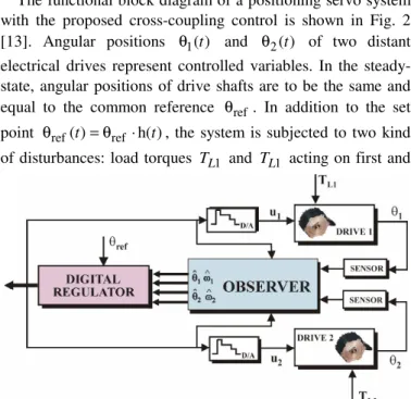
positioning systems into a high-accuracy robust tracking systems by using active compensators (ACs). Since a conventional system needs to be improved in tracking capability as well as in disturbance rejection, two digital ACs are introduced. The first AC represents feedforward improvement of tracking. The second AC is actually the ADE [9,13] that compensates system disturbances and is located in a local feedback loop. These digitally implemented ACs involve an active control substructure based on discrete-time sliding mode control (DSMC). In the paper the proposed control extension is described in details, DSM controller design procedure is explained and simulation tests on DC motor are presented.
II. IDEAL TRACKING SYSTEM
The well-known control structure with feedforward and disturbance compensations is shown in Fig.1 in digital realization. Under certain conditions this structure can ensure the output signal to ideally track the reference.
According to the structure in Fig. 1, the error signal may be easily expressed in complex domain with respect to reference and disturbance :
) ( ) ( 1 ) ( ] 1 ) ( ) ( [ ) ( )] ( ) ( 1 [ ) ( z G z G z D z G z G z R z G z G z E r dc fc + − + −
= . (1)
Ideal tracking occurs when the tracking error is annulated )
0 ) (
(ek = , which is the case when it holds
) ( ) ( ) ( )
( 1 1
z G z G z G z
Gfc dc
−
− ∧ =
= . (2) Hence, in order to achieve ideal tracking it is necessary that the transfer functions of the feedforward and disturbance compensators represent plant inverse dynamics. This requirement inevitably raises the following questions:
- how to obtain the information about disturbance if it is not available for direct measurement?
- how to overcome plant parameters uncertainty and variations as well as unmodeled dynamics.?
- how to realize plant inverse dynamics, since it is not a causal system?
The answers to these questions are offered in the following consideration.
Information about external disturbances is practically impossible to obtain by direct measurement. Therefore it is necessary to estimate the disturbance for its compensation. One possible structure for disturbance estimation is presented in Fig. 2a. In this digital realization extraction of the equivalent disturbance q(k) is done using the nominal plant model Gn(z). Mismatch between the nominal model and real plant inevitably exists due to parameter variations and unmodeled dynamics. Hence, plant dynamics may be described as )) ( 1 )( ( )
(z G z G z
G = n +δ , (3)
where perturbations are limited by the multiplicative bound of uncertainty δG(ejωT) γ(ω),ω
[
0,π/T]
∈
≤ . The extracted
equivalent disturbance is obtained in the form ) ( ) ( ) ( ) ( )
(k d k G z G z u k
q = + n δ k , (4) indicating that the equivalent disturbance carries information about external disturbance, which can always be mapped onto plant output, and parameter perturbations and unmodeled dynamics, i.e. internal disturbances.
According to Fig. 2a, plant output as a function of control and disturbance may be expressed as
) ( ) ( ) ( ) ( 1 ) ( ) ( 1 ) ( ) ( ) ( ) ( 1 )) ( 1 )( ( ) ( z D z G z G z G z G z G z U z G z G z G z G z G z Y n k n k n k n δ δ δ + − + + + = (5)
If the compensation filter Gk(z) represents nominal plant
Fig. 1. Block scheme of ideal tracking system: P-plant; C-main controller; DC-disturbance compensator; FC-feedforward compensator.
a) b) Fig. 2. a) Disturbance estimator; b) ADE based on DSMC.
inverse dynamics, i.e. G (z) G 1(z)
n k
−
= , output becomes )
( ) ( )
(z G zU z
U = n , which shows that all disturbances are completely eliminated and that the nominal plant behavior is ensured. Unfortunately, such filter is non-causal and cannot be realized.
Solution is proposed in [9] through the concept of ADE, Fig. 2b, where passive filter is replaced by an actively controlled subsystem. If DSM controller within ADE provides
) ( ) ( ˆ k qk
q = , i.e. ensures an ideal DSM regime, then controller output may be described as ( ) 1( ) ( )
z Q z G k
Usm = n− , showing that this subsystem acts as nominal plant inverse dynamics. Thus, complete disturbance rejection is achieved nominal plant behavior is secured. This way transforms the disturbance compensation problem into tracking problem of the referent signal q(k). In the tracking subsystem of ADE, DSM controller governs nominal model, not the real plant, so there are not any uncertainties and all state coordinates are available. Generally, due to the not known in advance referent signal
) (k
q it is possible to establish only quasi-sliding regime [15],
resulting in nonideal disturbance rejection. However, since DSMC systems provide high-accuracy tracking, an excellent compensation may be expected, i.e. near nominal behavior.
B. Active Compensators
The notion from ADE may also be used in realization of inverse dynamics that is required by the feedforward compensator FC in Fig. 1, which should improve reference tracking capacity of the system. Theoretically designed structure in Fig. 1 may be practically realized as shown in Fig. 3.
Disturbance compensator DC is actually an observer variant of ADE, which is formed by optimization of the structure in Fig. 2b. If DSM controller within FC establishes discrete sliding mode, then it holds ( ) 1( ) ( )
1 z G z R z
Usm = n− , which shows that FC acts as nominal model inverse dynamics. Since DC ensures plant nominal behavior, the resulting system exhibits ideal tracking of arbitrary referent signal. This control extension is suitable for the upgrade of already existing systems, whose main conventional controller Gr, usually PD
type, gives modest performance in tracking of complex signals in the presence of disturbances. Retuning of the main controller is not necessary, since the proposed control structure requires the main controller to be designed for the nominal plant, which is already the case in the practice.
Although it is known that SMC systems need measurement of all state coordinates, such system expansion does not require any additional sensors. Only input/output measurements are required, since ACs contain nominal models, which provide necessary state information for the DSM controllers. Stability of the overall system is secured by the occurrence and existence of the sliding regimes in the DSMC subsystems.
III. DSMCDESIGN
Both DSM controllers within KP and PK govern the nominal model and may be identical. The priority is to ensure as accurate tracking as possible in order to gain the precise nominal model inverse dynamics. Good results were obtained using DSMC algorithm [14], which guaranteed ideal tracking of parabolic signals. This control algorithm is based on the algorithm [16] enriched with the introduction of additional integral action with respect to the switching variable. Integration is activated only in the predefined vicinity of the sliding surface. Emergence of chattering, extremely undesirable phenomenon in SMC systems, is eliminated by imposing a linear control zone near the sliding surface [16]. Since the exposed control algorithm has been thoroughly elaborated in [14] and [13], it will be briefly described hereafter.
Let the nominal plant model be in the form
1 2
1 2
1 0 ,ˆ
0 1 0 x q u u b x x a x x sm
sm = + =
+ −
= x Ax b . (6)
It is a second order model representing the mechanical subsystem dynamics of an electromechanical positional system. The dynamics of the electrical part, i.e. electric drive, is neglected since it is much faster than the mechanical counterpart. Tracking error may be calculated as
) ( ) ( ) ( ˆ ) ( )
(t qt qt qt x1 t
e = − = − . The model (6) may be transformed into the tracking error space
+ = = = = + − = q q a e e e e
usm , , 0
2 1 p e p b Ae
e . (7)
Unlike the previous model, a disturbance vector p occurs in this model as a consequence of variability of the input signal q.
The first component aq scan be easily compensated since
forming of e2 already needs knowledge of q, which may be
obtained using a differentiator. However, q cannot be reliably
obtained by twofold differentiation due to drastic amplification of noises. Hence, vector p=[0 q]T may be regarded as a
disturbance vector. The discrete-time model of the system (7) for the given sampling period T is obtained in the form
. )d ( ; d ; / , / , / ) ( ), ( ) ( ) ( ) ( ) 1 ( 0
0 = +
= = = = − = + − + = + T t d T t d T d d d d sm t T-t kT t e T T T k T k u T k T k e k p e d b e b A d d b b I A A d b e A e A A A δ δ δ δ δ δ (8)
Control task is to annul the tracking error, i.e. the trajectories of the system (8) should reach state space origin. Using the concept of DSMC this would mean that system trajectories from an arbitrary initial point should reach in finite time the sliding line s(k)=0, defined by the switching function
] [ ), ( )
(k δ k δ cδ1 cδ2
s =c e c = , (9) and continue to slide along the line into the origin, which would result in ideal tracking. System dynamics in the sliding mode is strictly defined by the sliding line vector cδ, which should be chosen according to the desired dynamics.
which is accomplished according to (9) and (8) by the following control ) ( ) ( ) ( ) ( 1 s T k k k
usm = + + −Φ
δ δ δ
δA e c d
c (11) under normalization cδbδ =1. This control is not feasible due to unknown dδ, that is q. A feasible control
)) ( sgn( } |, ) ( min{| ) ( )
(k k T 1 sk T s k
usm =cδAδe + − σ (12) gives the following reaching dynamics.
) ( )) ( sgn( } |, ) ( min{| ) ( ) 1
(k s k sk T s k T k
s + − =− σ + cδdδ . (13)
It is evident that control (12) has two modes: nonlinear and linear. Nonlinear control
)) ( sgn( ) ( ) (
_ k k s k
usm n =cδAδe +σ (14)
acts outside the zone |s(k)|<σT , which produces the reaching dynamics given by
) ( )) ( sgn( ) ( ) 1
(k s k T s k T k
s + − =−σ + cδdδ . (15) To ensure the reaching of the sliding line, the condition
0 ) ( )] ( ) 1 (
[s k+ −sk s k < must be satisfied. Under assumption
that the reference is a smooth function, its second derivative is bounded |q|≤Mr and therefore the disturbance is also bounded ||dδ ||≤M . Reaching is secured if the switching gain
σ fulfills inequality σ >||cδ ||M . It means that the system trajectories will enter zone |s(k)|<σT in finite number of steps.
Inside this zone, the control signal is linear ) ( ) ( ) ( 1
_ k k T s k
usm l =cδAδe + − , (16) which provides s(k+1)=Tcδdδ(k), indicating that a quasi-sliding mode arises in a single step within a domain described by } || || | ) ( |
{ s T M
Sqs= e e ≤ cδ . (17) For small sampling periods T the width of the quasi-sliding
domain is also small, which guarantees high-precision tracking. If the referent signal is q is a constant or a ramp
function, the second component of the disturbance is zero, 0
=
q , which gives p=bd =bδ =M =0. It yields s(k+1)=0,
that is, ideal discrete sliding mode occurs in one step that provides ideal tracking of ramp references. The control (16) is the so called equivalent control ueq.
Further tracking improvement was suggested in [14] by introduction of the supplemental integral action with respect to switching variable s(k). Namely, integration is activated only
inside the linear control zone, only when the tracking error is small, i.e. in the sliding mode final stage. Activation of the integral action within the nonlinear control zone or distant from the origin is completely unnecessary and may can produce an unwanted overshoot. This idea is described by the following expression ≤ − + > > = , || ) ( || ), 1 ( ) ( 0, || ) ( || , 0 ) ( ρ ρ k k u k hs k k u I I e
e (18)
where ρ is a small positive constant. Integral gain h should
DSM controller, created by merging the described control components, is summarized by
< ∩ < + ≤ > = . || ) ( || | ) ( | ), ( ) ( , | ) ( | ), ( , | ) ( | ), ( ) ( _ _ _ ρ σ σ σ k T k s k u k u T k s k u T k s k u k u I l sm l sm n sm sm e (19)
Because of the introduced additional integral action, which increases tracking accuracy, the designed DSM controller provides ideal tracking of parabolic signals.
Since the main controller is already tuned by some conventional method, it remains to define AC sliding mode dynamics, which is prescribed by the selection of vector cδ. In
case of a second order system in sliding mode, due to the order reduction of the differential equation that describes sliding mode dynamics, a single eigenvalue T
e
z1= −α determines
desired system dynamics. The desired slope α of the sliding line is established if it holds
α
δ δ δ
δb =1 ∧ c1/c2 =
c . (20) The procedure for the calculation of vector cδ in case of higher order systems is given in [16].
IV. SIMULATION EXAMPLE
Permanent magnet direct current motor is considered as a plant, whose nominal mode is given by
1 2 1 2 1 , 1 0 654 0 5 . 26 0 1 0 x y f u x x x x = + + −
= . (21)
Sampling period is T=0.4 ms. Parameters of the DSM
controllers within ACs are set as: α=50; h=100 in DC and h=1000 in FC; σ=10; ρ=0.01; [7.557248 0.151449]10−2
δ=− ⋅
c .
Differentiator [12] is employed to obtain the derivatives of the input signals r and q. The main controller is a PD controller
that is tuned by the following selection of the well-known parameters: Kr=25 and Td=1/26.5 s. The input signal that
represents angular position reference is described by
r(t)=5[cos(t)-cos(2.5t)]. Load torque that acts as an external
disturbance is expressed by f(t)=200[h(t-5)-h(t-10)]+
+20sin(5t)h(t-12), where h(t) represents step function.
Tracking errors obtained by simulations in case of different configurations are given in Fig. 4.
V. CONCLUSION
The paper proposes a way to upgrade conventional servo-systems by introduction of digital ACs. Adjoining of DC and FC improves system performances in reference tracking as well as disturbance rejection. Both compensators contain active DSM controlled subsystems, whose controllers are designed for the nominal plant. Simulation results evidently show that the proposed control extension ensures superior performance comparing to the initial system, confirming that a conventional positioning system becomes a robust high-performance tracking system.
REFERENCES
[1] T. Umeno, T. Hory, “Robust speed control of DC servomotors using modern two degrees-of-freedom controller design,” IEEE Trans. Ind. Electron., Vol. 38, No. 5, pp. 363-368, 1991.
[2] T. Umeno, T. Kaneko, Y. Hory, “Robust servosystem design with two degrees of freedom and its application to novel motion control of robot manipulators, ” IEEE Trans. Ind. Electron., Vol. 40, No. 5, pp. 473-485, 1993.
[3] Y. Fujimoto, A. Kawamura, “Robust servo-system based on two-degree-of-freedom control with sliding mode”, IEEE Trans. Ind. Electron., Vol. 42, No. 3, pp. 272-280, 1995.
[4] H. Fujimoto, Y. Hori, A. Kawamura, “Perfect tracking control based on multirate feedforward control with generalized sampling periods,” IEEE Trans. Ind. Electron., Vol. 48, No. 3, pp. 636-644, 2001.
[5] H. Fujimoto, Y. Hori, “High-performance servo systems based on multirate sampling control,” Control Engineering Practice, Vol. 10, pp. 773-781, 2002.
[6] V.I. Utkin, Sliding modes in control and optimization, Springer-Verlag, 1992.
[7] B. Draženovi , “The invariance conditions in variable structure systems”, Automatica, Vol. 5, pp. 287-295, 1969.
[8] . Milosavljevi , N. Mihajlovi , G. Golo, “Static accuracy of the variable structure system," Proc. 6th Int. SAUM Conference on Systems Automatic Control and Measurements, Niš, Yugoslavia, pp. 464–469, 1998.
[9] B.Veseli , . Milosavljevi , B. Peruni i -Draženovi , D. Miti , “Digitally controlled sliding mode based servo-system with active disturbance estimator,” Proc. IEEE 9th Int. Workshop on Variable Structure Systems (VSS2006), Algero, Italy, pp. 51-56, 2006.
[10] A. Damiano, G.L. Gatto, I. Marongiu, A. Pisano, “Second-order sliding-mode control of DC drives”, IEEE Trans. Ind. Electron., Vol. 51, No. 2, pp. 364-373, 2004.
[11] A. Levant, “Robust exact differentiation via sliding mode technique”, Automatica, Vol. 34, No. 3, pp. 379-384, 1998.
[12] J.X. Xu, J. Xu, R. Yan, “On sliding mode derivative estimators via closed-loop filtering,” Proc. IEEE 8th Int. Workshop on Variable Structure Systems (VSS2004), Vilanova i la Geltru, Spain, 2004. [13] B. Veseli , B. Peruni i -Draženovi , . Milosavljevi ,
“High-performance position control of induction motor using discrete-time sliding-mode control,” IEEE Trans. Ind. Electron., Vol. 55, No. 11, pp. 3809-3817, 2008.
[14] . Milosavljevi , B. Peruni i -Draženovi , B. Veseli , D. Miti , “A new design of servomechanisms with digital sliding mode,” Electrical Engineering, Vol. 89, No. 3, pp. 233-244, 2007.
[15] . Milosavljevi “General conditions for the existence of a quasi-sliding mode on the switching hyperplane in discrete variable structure systems,” Automatic Remote Control, Vol 46, pp. 307-314, 1985. [16] G. Golo, . Milosavljevi , “Robust discrete-time chattering free sliding
mode control,” Systems & Control Letters, Vol. 41, pp. 19-28, 2000. Line Main controller DC FC
1 On Off Off
2 On On. Off
3 On Off On
4 Off On On
5 On On On
Abstract—Algorithms for efficiency optimized control of
induction motor drives are presented in this paper. As a result, power and energy losses are reduced, especially when load torque is significant less compared to its rated value. According to the literture, there are three strategies for dealing with the problem of efficiency optimization of the induction motor drive: Simple State Control, Loss Model Control and Search Control. Basic characteristics each of these algorithms and their implementation in induction motor drives are described. Moreover, induction motor drive is often used in a high performance applications. Vector Control or Direct Torque Control are the most commonly used control techniques in these applications. These control methods enable software implementation of different algorithms for efficiency improvement. Simulation and experimental tests for some algorithms are performed and results are presented.
Index Terms—Induction motor, efficiency optimization,
dynamic programming.
I. INTRODUCTION
NDOUBTEDLY, the induction motor is a widely used electrical motor and a great energy consumer. Three-phase induction motors consume more than 60% of industrial electricity and it takes a lot of effort to improve their efficiency [1]. The vast majority of induction motor drives are used for heating, ventilation and air conditioning (HVAC). These applications require only low dynamic performance and in most cases only voltage source inverter is inserted between grid and induction motor as cheapest solution. The classical way to control these dives is constant V/f ratio and simple methods for efficiency optimization can be applied [2]. From the other side in applications like electric vehicle energy has to be consumed in the best possible way and use of induction motors in such application requires an energy optimized control strategy [3]. Also, there are many high performance industrial drives which operate in periodic cycles. In these cases implementation of efficiency optimization algorithm are more complex.
In a conventional setting, the field excitation is kept constant at rated value throughout its entire load range. If machine is under-loaded, this would result in over-excitation
B. D. Blanuša and B. L. Doki are with the Faculty of Electrical Engineering, University of Banja Luka, Banja Luka, Bosnia and Herzegovina.
S. N. Vukosavi is with the Faculty of Electrical Engineering, University of Belgrade, Belgrade, Serbia.
and unnecessary copper losses. Thus in cases where a motor drive has to operate in wider load range, the minimization of losses has great significance. It is known that efficiency improvement of induction motor drive (IMD) can be
implemented via motor flux level and this method has been proven to be particularly effective at light loads and in a steady state of drive. Moreover, induction motor drive is often used in servo drive applications. Vector Control (VC) or Direct
Torque Control (DTC) are the most commonly used control
techniques in such applications and these methods enable software implementation of different algorithms for efficiency improvement.
Functional approximation of the power losses in the vector controlled induction motor drive is given in the second Section. Strategies for efficiency optimization of IMD and their basic characteristics are described in third section. Qualitative analysis and comparison of interesting algorithms for efficiency optimization with simulation and experimental results are presented in fourth section. Brief description of efficiency optimized control of high performance IMD is described in fifth section.
II. FUNCTIONAL APPROXIMATION OF THE POWER LOSSES IN THE INDUCTION MOTOR DRIVE
The process of energy conversion within motor drive converter and motor leads to the power losses in the motor windings and magnetic circuit as well as conduction and commutation losses in the inverter [4].
Converter losses: Main constituents of converter losses are the
rectifier, DC link and inverter conductive and inverter commutation losses. Rectifier and DC link inverter losses are proportional to output power, so the overall flux-dependent losses are inverter losses. These are usually given by:
(
2 2)
2
q d INV s INV
INV
R
i
R
i
i
P
=
⋅
=
⋅
+
, (1)where id,, iq are components of the stator current is in d,q
rotational system and RINV is inverter loss coefficient.
Motor losses: These losses consist of hysteresis and eddy
current losses in the magnetic circuit (core losses), losses in the stator and rotor conductors (copper losses) and stray losses. The main core losses can be modeled by:
2 2 2
e m e e m h
Fe c c
P = Ψ ω + Ψ ω , (2)
where ψd is magnetizing flux, ωe supply frequency, ch is
hysteresis and ceeddy current core loss coefficient.
Efficiency Optimized Control of High
Performance Induction Motor Drive
Branko D. Blanuša, Branko L. Doki , and Slobodan N. Vukosavi
Copper losses are due to flow of the electric current through the stator and rotor windings and these are given by:
2 2
q r s s
Cu Ri R i
p = + , (3)
The stray flux losses depend on the form of stator and rotor slots and are frequency and load dependent. The total secondary losses (stray flux, skin effect and shaft stray losses) usually don't exceed 5% of the overall losses [4].
III. STRATEGIES FOR EFFICIENCY OPTIMIZATION OF IMD Numerous scientific papers on the problem of loss reduction in IMD have been published in the last 20 years. Although
good results have been achieved, there is still no generally accepted method for loss minimization. According to the literature, there are three strategies for dealing with the problem of efficiency optimization of the induction motor drive [5]:
− Simple State Control - SSC ,
− Loss Model Control - LMC and
− Search Control- SC.
The first strategy is based on the control of one of the variables in the drive [5-7] (Fig. 1). This variable must be measured or estimated and its value is used in the feedback control of the drive, with the aim of running the motor by predefined reference value. Slip frequency or power factor displacement are the most often used variables in this control strategy. Which one to chose depends on which measurement signals is available [5]. This strategy is simple, but gives good results only for a narrow set of operation conditions. Also, it is sensitive to parameter changes in the drive due to temperature changes and magnetic circuit saturation.
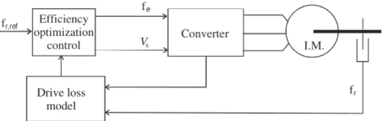
In the second strategy, a drive loss model is used for optimal drive control [4,8] (Fig. 2). These algorithms are fast because the optimal control is calculated directly from the loss model. But, power loss modeling and calculation of the optimal operating conditions can be very complex. This strategy is also sensitive to parameter variations in the drive.
In the search strategy, the on-line procedure for efficiency optimization is carried out [9-11] (Fig. 3). The optimization variable, stator or rotor flux, increases or decreases step by step until the measured input power is at a minimum. This strategy has an important advantage over others: it is insensitive to parameter changes.
Also, there are hybrid methods which include good characteristics of different strategies for efficiency improvement [10].
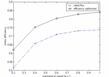
The published methods mainly solve the problem of efficiency improvement for constant output power. Results of applied algorithms highly depends from the size of drive (Fig. 4) [2] and operating conditions, especially load torque and speed (Figs. 5 and 6). Efficiency of IM changes from 75% for low power 0,75kW machine to more than 95% for 100kW machine. Also efficiency of drive converter is typically 95% and more.
That’s obvious, converter losses is not necessary to consider in efficiency optimal control for small drives. Also, these algorithms for efficiency optimization give best result in power losses reduction for a light loads and in a steady state.
IV. COMPARISON OF SOME ALGORITHMS FOR EFFICIENCY
OPTIMIZATION OF IMD
Selection of algorithm for efficiency optimization depends from many factors, drive features, operating conditions, measuring signals, drive control and etc.
If the losses in the drive were known exactly, it would be possible to calculate the optimal operating point and control of drive in accordance to that. For the following reasons it is not possible in practice [9]:
Optimal state reference
Control Converter f
V I.M.
Control state variable (measured or estimated)
e
s
fr
Fig. 1. Control diagram for the simple state efficiency.
Converter f
V I.M.
e
s
fr,ref Efficiency
optimization control
fr
Drive loss model
Fig. 2. Block diagram for the model based control strategy.
Control Converter
f
V I.M.
e
s
fr Power loss
calculation
fr,ref
P -inPout
P =γ P γ
ψr ψ
r,min
Fig. 3. Block diagram of search control strategy.
Fig. 4. Rated motor efficiences for ABB motors (catalog data) and typical converter efficiency.
− A number of fundamental losses are difficult to predict: stray load, iron losses in case of saturation changes, copper losses because of temperature rise etc.
− Due to limitation in costs all the measurable signals cannot be acquired. It means that certain quantities must be estimated which naturally leads to an error.
Two interesting algorithms SC and LMC are discussed and
their results in efficiency optimization are compared for different operating conditions. Also, power losses for these algorithms are presented together with a case when motor is excited by rated magnetizing flux. Operation of drive has been tested under following operating conditions. There are three intervals: acceleration from 0 to ωref, interval [0, t1], constant
speed ω=ωref , interval [t1, t2], deceleration from ωref to 0,
interval [t2, t3]. Load torque changes at the moment t4=5s from
0.4 p.u. to 1.05 p.u. and vice versa at the moment t5=10s for a
constant reference speed of ωref=0.6 p.u. (Fig.7). The steep
change of load torque appears with the aim of testing the drive behavior in the dynamic mode and its robustness within sudden load perturbations.
Simulation tests show that LMC algorithm is faster than SC algorithm and gives better result in power loss reduction than SC algorithm. Optimal magnetizing flux is derived directly from the loss model of IMD. Loss modeling, optimal flux calculation and especially its sensitivity to parameter changes are problems which limits implementation of this control strategy. But LMC algorithm with on-line parameter identification in the loss model and hybrid models make this strategy very actual [4].
From the other side search strategy optimization does not require the knowledge of motor parameters and the algorithm is applicable universally to any motor. Besides all good characteristics of search strategy methods, there is an outstanding problem in its use. Flux in small steps oscillates around its optimal value. Torque ripple appears each time the flux is stepped. Sometimes convergence to its optimal value is to slow, so these methods are not applicable for high performance drives. There are numerous papers which treats problem of step size in the magnetization flux for SC algorithms. Fuzzy or neuro-fuzzy controllers are often used to obtain smooth and fast flux convergence during optimization process [9,10].
V. EFFICIENCY OPTIMIZATION IN DYNAMIC OPERATION
There is an interesting question to ask, how algorithms for efficiency optimization can be applied in the dynamic mode and what are problems and constrains. There are two distinctive cases: when the operation conditions are not known in advance and when they are.
In the cases when the operating conditions are not known in advance (e.g. electrical vehicles, cranes, etc.), it is important to watch for the electromagnetic torque margin and energy saving presents a compromise between power loss reduction and dynamic performances of the drive [12].
There are two common approaches when operation conditions are known in advance:
Fig. 5. Measured standard motor efficiencies with both rated flux and efficiency optimized control at rated mechanical speed (2.2 kW rated power).
Fig. 6. Measured standard motor efficiencies with both rated flux and efficiency optimized control at light load (20% of rated load).
Fig. 7. Comparison of SC and LMC algorithms for efficiency optimization in IMD.
a) Steady state modified [13,14] and b) Dynamic programming [13-15].
In the first case, the same methods, LMC or SC controllers, are used for steady state as well. Magnetizing flux is set to its nominal value during the dynamic transition [13], or a fuzzy controller is used to adjust the flux level in a machine by operation conditions [13, 14]. This can be realized in cases when torque or speed response is not so important (e.g. elevators or cranes).
If the both high dynamic performance and losses minimization are required dynamic optimization is necessary. By using the dynamic programming approach, optimal control is computed so that the drive runs with minimal losses. Torque and speed trajectories have to be known in advance and flux trajectory has to be computed off-line, which requires a lot of processing time.
Also, an interesting problem is how to minimize energy consumption of IMD when it works in a periodic cycles. Closed-cycle operation is often for robots and other high performance industry machines. Efficiency optimized control for closed-cycle operation of high performance IMD, based on dynamic programming approach is applied.
Following dynamic programming approach, performance index, system equations, constraints and boundary conditions for a vector controlled IMD in the rotor flux oriented reference frame, can be defined as follows:
a) The performance index is [12, 16]:
( )
[
]
− = + + + = 1 0 2 2 2 2 1 22 () () () () ()
N i D e D e q
d i bi i c i i c i i
ai
J ω ψ ω ψ , (1)
where id , iq: d and q are components of the stator current vector,
ψD is rotor flux and ωeissupply frequency. The a, b, c1and c2 are
parameters in the loss model of the drive. These parameters are determined through the process of parameter identification [4,12]. Rotor speed ωr and electromagnetic torque Tem are defined by
operating conditions (speed reference, load and friction).
b) The dynamics of the rotor flux can be described by the following equation:
(
1)
( )
1 s s( )
D D m d
r r
T T
i i L i i
T T
ψ + =ψ − + , (2)
where Tr=Lr/Rr is a rotor time constant.
c) Constraints:
( ) ( )
( )
( )
( )
( )
( )
0
.
)
(
,
0
)
(
,
)
(
,
0
)
(
,
2
2
3
,
min 2 max 2 2 2≤
≤
−
≤
≤
−
≤
−
+
=
=
−i
flux
rotor
for
i
speed
for
current
stator
for
I
i
i
i
i
torque
for
L
L
p
k
i
T
i
i
i
ki
D D Dn D rn r rn s q d r m em q dψ
ψ
ψ
ψ
ω
ω
ω
(3)Ismax is maximal amplitude of stator current, ωrn is nominal
rotor speed, p is number of poles, ΨDmin is minimal and ΨDn
is nominal value of rotor flux.
Also, there are constraints on stator voltage:
,
0
2 2 maxs q
d
v
V
v
+
≤
≤
(4)where vd and vq are components of stator voltage and Vsmax is
maximal amplitude of stator voltage. Voltage constraints are more expressed in DTC than in field-oriented vector control.
d) Boundary conditions:
Basically, this is a boundary-value problem between two points which are defined by starting and final value of state variables:
( )
( )
( )
( )
( )
( )
)
3
(
,
0
,
0
0
,
0
0
in
constrains
g
considerin
free
N
N
T
T
N
Dn Dn em em r r=
=
=
=
=
=
ψ
ψ
ω
ω
(5)Presence of state and control variables constrains generally complicates derivation of optimal control law. On the other side, these constrains reduce the range of values to be searched and simplify the size of computation [17].
In a purpose to determine stationary state of performance index, next system of differential equations are defined:
( )
(
)
(
( )
( )
)
( )
( )
( ) ( )
( )
( ) ( )
(
)
( ) ( )
( )
( )
( )
( )
( )
,
1
,..,
2
,
1
,
0
,
0
1
2
0
2
2
1
2 2 1−
=
+
=
=
=
+
+
+
=
+
+
+
−
+
=
N
i
i
i
i
T
L
i
i
i
T
i
i
i
ki
L
T
T
i
i
ki
i
i
ai
i
ki
i
i
bi
i
i
c
i
c
T
T
T
i
i
D q r m r e em q d m r S q d d q D e e r S rψ
ω
ω
λ
µ
µ
ψ
ω
ω
λ
λ
(6)whereλ and µ are Lagrange multipliers.
By solving the system of equations (6) and including boundary conditions given in (5), we come to the following system [16]:
( )
( )
(
)
( )
( )
( )
( )
( )
( )
( )
(
( )
( )
)
( )
(
)
.
1
,..,
2
,
1
,
0
1
2
,
,
)
(
)
(
1
2
)
(
)
1
(
)
(
2
2 2 1 2 2 3 4−
=
−
+
+
+
=
+
=
=
−
−
+
−
=
=
+
+
N
i
T
T
T
i
i
i
c
i
c
i
i
i
i
T
L
i
i
i
ki
i
T
i
i
i
i
L
T
T
T
i
T
T
T
i
i
T
k
b
i
i
T
T
i
i
ai
r s r D e e D q r m r e d em q d m s r s D s r r D em d r S dλ
ψ
ω
ω
λ
ψ
ω
ω
ψ
ψ
λ
(7)Every sample time values of ωr(i) and Tem(i) defined by
operating conditions is used to compute the optimal control (id(i), iq(i), i=0,..,N-1) through the iterative procedure and applying the
backwardprocedure, from stage i =N-1 down to stage i =0. For
the optimal control computation, the final value of ψD and λ have
to be known. In this case, ψD(N)=ψDmin and
( )
0
.
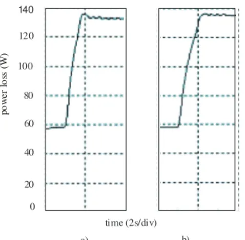
especially for low flux level. Therefore, some experiments are made to appraise speed response on steep increase of load for LMC and optimal flux control method (Fig. 8).
The method for efficiency optimization based on the dynamic programming approach should show good results regarding the loss reduction during transient processes. Thus, it is very important to measure power losses in the drive for this method during the transient process and compare it with other efficiency optimization methods. The graphic of power losses for steep increase of load torque for optimal flux and LMC method is shown in Fig. 9.
Simulation and experimental tests are performed for typical closed-cycle operation, although this algorithm can be applied regardless of IMD operating conditions.
VI. CONCLUSION
Algorithms for efficiency optimization of IMD are briefly described and some comparison between LMC and SC strategies are made. Also, one procedure for efficiency optimization in dynamic operation based on dynamic programming approach has been applied. According to the performed simulations and experimental tests, we have arrived at the following conclusions:
algorithm for efficiency optimization is applied or not. For a light load algorithm based on optimal flux control gives significiant power loss reduction when drive works with its nominal flux (Figs. 5, 6 and 7).
2. For a steady state, power losses are practically same for both methods, SC and LMC, but SC algorithms give faster convergence of magnetizing flux during transient prosess and consequently less energy consumption. (Fig. 7). From the other side SC algorithms do not require knowledge of motor parameters and not sensitive to motor parameters changes.
3. Optimal flux control based on dynamic programming gives better dynamic features and less speed drops on steep load increase, then LMC methods (Figs. 8 and 9). The obtained experimental results show that this algorithm is applicable. It offers significant loss reduction, good dynamic features and stable operation of the drive. One disadvantage of this algorithm is its off-line control computation.
REFERENCES
[1] S. N. Vukosavic,” Controlled electrical drives - Status of technology” Proceedings of XLII ETRAN Conference, No. 1, pp. 3-16, June 1998. [2] F. Abrahamsen, F. Blaabjerg, J.K. Pedersen, P.Z. Grabowski and P.
Thorgensen,” On the Energy Optimized Control of Standard and High Efficiency Induction Motors in CT and HVAC Applications”, IEEE Transaction on Industry Applications, Vol.34, No.4, pp.822-831, 1998. [3] M.Chis, S. Jayaram, R. Ramshaw, K. Rajashekara:” Neural network
based efficiency optimization of EV drive”, IEEE-IECIN Conference Record, pp. 454-457, 1997.
[4] S.N. Vukosavic, E Levi:”Robust DSP-based efficiency optimization of variable speed induction motor drive”, IEEE Transaction of Ind. Electronics, Vol.50, No.3, pp. 560-570, 2003.
[5] F. Abrahamsen, J.K. Pedersen and F. Blaabjerg: ”State-of-Art of optimal efficiency control of low cost induction motor drives” Proceedings of PESC’96, pp. 920-924, 1996.
[6] T. Hatanaka, N. Kuwahara: Method and apparatus for controlling the supply of power to an induction motor to maintaining in high efficiency under varying load conditions, U.S. Patent 5 241 256, 1993.
[7] M.E.H. Benbouzid and N.S. Nait Said, ”An efficiency-optimization controller for induction motor drives”, IEEE Power Engineering Review, Vol. 18, Issue 5, pp. 63 –64, 1998.
[8] F. Fernandez-Bernal, A. Garcia-Cerrada and R. Faure: “Model-based loss minimization for DC and AC vector-controlled motors including core saturation”, IEEE Transactions on Industry Applications, Vol. 36, No. 3, pp. 755 -763, 2000.
[9] G. C. D. Sousa, B. K. Bose, J. G. Cleland, “Fuzzy Logic Based On-Line Efficiency Optimization of an Indirect Vector-Controlled Induction Motor Drive“, IEEE Trans. Ind. Elec., Vol.42, No.2, 1995.
[10] D.A. Sousa, Wilson C.P. de Aragao and G.C.D. Sousa: ”Adaptive Fuzzy Controller for Efficiency Optimization of Induction Motors”, IEEE Transaction on Industrial Electronics, Vol. 54, No.4, pp. 2157-2164, 2007.
[11] Ghozzy S., Jelassi K., Roboam X.:” Energy optimization of induction motor drive”. International Conference on Industrial Technology, Conference Record of the 2004 IEEE, pp. 1662 -1669, 2004. [12] B. Blanusa, P. Mati , Z. Ivanovic and S.N. Vukosavic: ” An Improved
Loss Model Based Algorithm for Efficiency Optimization of the Induction Motor Drive”, Electronics, Vol.10, No.1, pp. 49-52, 2006. [13] E. Mendes, A.Baba, A. Razek:” Losses minimization of a field oriented
controlled induction machine”, Electrical Machines and Drives, Seventh International Conference on (Conf. Publ. No. 412), pp. 310 -314, 1995. [14] J. Moreno, M. Cipolla, J. Peracaula, P.J. Da Costa Branco:”Fuzzy logic
based improvements in efficiency optimization of induction motor drives” , Proceedings of the Sixth IEEE International Conference on Fuzzy Systems, Vol. 1, pp. 219 -224, 1997.
0 1.0
0.8
0.6
0.4
0.2
m
ec
ha
ni
ca
l s
pe
ed
p
.u
.
a) time (2s/div)
b) time (2s/div)
Fig. 8. Speed response on steep load change for a) LMC method, b) optimal flux.
140
120
100
80
60
40
20
a)
time (2s/div) b)
po
w
er
lo
ss (
W
)
0
Fig. 9. Graph of power losses during dynamic operation for a) LMC method, b) optimal control.
[15] R. D. Lorenz, S.-M. Yang:” Efficiency–optimized flux trajectories for closed-cycle operation of field-orientation Induction Machine Drives” IEEE Transactions on Industry Applications , Vol.28, No.3, pp. 574-580, 1992.
[16] B. Blanusa and S. N. Vukosavic:”Efficency Optimized Control for Closed-cycle Operations of High Performance Induction Motor Drive”, Journal of Electrical Engineering, Vol. 8 Edition: 3, pp. 81-88, 2008. [17] Brayson A. E., Applied Optimal Control,Optimization, Estimation and
Abstract—In this paper developement of an acquisition system
(AS) for static torque characteristics of electrical machines measuring is described. AS is implemented on the device „Dr.Staiger, Mohilo+CoGmbH” using acquisition card with appropiate software. Performances of the new system are illustrated by few representative measurements.
Index Terms—Static Torque Characteristics, Machine Testing, Measuring and acquisition.
I. INTRODUCTION
EASUREMENT and acquisition of the torque of electric machines is one of the most difficult machines inspections. Test system must have the capability to drive machine in investigated operating mode (burden state) while a torque transducer, for direct measurements is sophisticated, delicate and expansive device. Regarding that, torque measuremets of machine in burden state are, in most all events, performed in specialized test laboratories, mostly as a standard testing [1-3].
True torque value is required information for electric machine construction in order to determine whether the tested machine reaches its projected performance, to determine operating characteristics, as well as in standardization to identify if tested machine satisfies designated standard. In modern electric motor drive, torque is estimated (calculated) with accessible gauge measurements (current and voltage), but the only way to determinate exact value of torque on motor spindle is direct measurement. Torque measurement domain is covered by the appropriate regulations. [1-4]
Torque characterisitcs are represented with torque conditionality on machine speed, on machine spindle (or indirectly, conditionality of time).
Existing equipment for recording torque characteristics is due to the price and complexity, for many years held in use. Improvement technologies, primarily measurement - acquisition systems, the existing devices are exceeded. In such cases, it is very cost-effective to renovate measurement-acquisition systems, by the retention of burden system. In this
G. Vukovi , S. Ajkalo, and S. Joki are with the Faculty of Electrical Engineering, University of East Sarajevo, East Sarajevo, Bosnia and Herzegovina.
P. Mati , is with the Faculty of Electrical Engineering, University of Banja Luka, Banja Luka, Bosnia and Herzegovina.
way, the existing set of equipment (torque encoders and burden system) are still in use, and allows the direct processing of measured data on the computer.
In this paper, just such a procedure is described, in which the measurement system of outdated technological device for torque measurements is changed with contemporary system. First described is the torque sensor with burden system, and hardware and software of a new measurement - acquisition system. After that, follow the pictures of important torque characteristics that serve to illustrate the performance of projected system. At the end are the guidelines for further work.
II. DESCRIPTION OF THE DEVICE AND PURPOSE
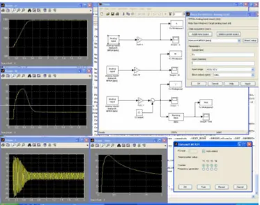
Analyzing device “Dr. Steiger, Mohilo+CoGmbH” is intended for inspection and verification torque characteristics of electric machines and other rotation devices [5]. Block scheme of the device “Dr.Steiger,Mohilo+CoGmbH” with measurement-acquisition system is represented on Fig. 1.
Components of the device are measurement desk, burden system, and command-measurement desk. On the measurement desk is fixed machine under test and connected with one of three measurements spindles, depending on motor speed and power. Coupling between device and tested machine has been accomplished with special claw clutch. For each of the three spindles there are a couple of sensors for speed and torque measurements. Torque encoders are inductive and speed measurement is implemented with optical increment encoders. Spindles are getting out from a specific transmission box that allows various combinations of simultaneous or particular use
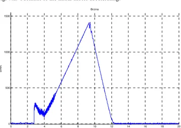
![Fig. 2. IFOC drive dynamic performance (top – estimated torque T e [Nm], bottom – speed m [rad/s])](https://thumb-eu.123doks.com/thumbv2/123dok_br/16432606.196096/23.918.72.443.534.894/fig-ifoc-drive-dynamic-performance-estimated-torque-speed.webp)