Nuno Crespo,
M. Paula Fontoura & Nádia Simões
Spatial centrality: an approach with sectoral
linkages
WP14/2014/DE/UECE _________________________________________________________
De pa rtme nt o f Ec o no mic s
W
ORKINGP
APERSSpatial centrality: an approach with sectoral linkages
(a), * Nuno Crespo, (b) M. Paula Fontoura, and (a)Nádia Simões
(a) Instituto Universitário de Lisboa (ISCTE – IUL), ISCTE Business School Economics Department, BRU – IUL (Business Research Unit), Lisboa, Portugal.
(b) Instituto Superior de Economia e Gestão (ISEG – Universidadede Lisboa), UECE (Research Unit on Complexity and Economics), Lisboa, Portugal.
* Author for correspondence. Av. das Forças Armadas, 1649-026 Lisboa, Portugal. E-mail: [email protected].
Abstract
This paper proposes a measure with six components to evaluate the degree of centrality (advantage) of a sector located in a region considering internal and external components and economic and geographical aspects. The main novelty of this indicator is that the definition of “mass” takes into consideration intra and inter-sectoral effects. In fact, the new economic geography has shown that a sector takes advantage of being in a particular location through two main channels: the proximity to other firms in the sector (intra-sectoral effects) and spillover effects arising from the proximity to upstream and downstream sectors (inter-sectoral effects). The two effects will be considered in both the region of location of the sector under analysis and in the other regions related to it. The hypothesis is that the spatial centrality of a sector varies positively with geographic proximity to firms in the same economic sector and in other sectors connected by vertical linkages and negatively with inter-regional distance. The index allows a double reading: it is possible to identify the sectors in which the region has a higher degree of centrality and the regions with a greater degree of centrality in this sector. To illustrate the method, we include an example for the Portuguese economy at the county level (275 regional units).
Acknowledgements
1. Introduction
One of the most important characteristics of economic activity is that it normally appears to be spatially concentrated. Since the early 1990s, with the work of Krugman (1991) and the subsequent new economic geography (NEG) models, the agglomeration of economic activity has emerged as a central issue in economic studies. According to these models, cumulative forces strengthened by the reduction of spatial transaction costs may create or reinforce polarized economic landscapes that contrast with increasingly peripheral areas. To encapsulate the real spatial economy there are many indicators. In general, the indicators available in the literature fall into two broad types: a group that measures the degree of concentration (agglomeration) of economic activity in a location unit (see, among others, Ellison and Glaser, 1997; Maurel and Sédillot, 1999; Duranton and Overmann, 2002); and a group comprising accessibility and peripherality (identical to low accessibility) indices, aiming to describe a particular location taking into account “opportunities, activities or assets in other areas and the area itself” (Wegener et al., 2002).1
The theme of accessibility has been increasingly invoked in recent years, in part due to the concern with regional performance and other factors that may lead to regional inequality.2 Firms seek to locate where the markets are. In fact, proximity to the markets is one of the location determinants traditionally included in many empirical studies. However, in most cases only the demand that is specific to the region/country under analysis is considered, i.e., the importance of neighboring spaces is ignored (Head and Mayer, 2004). On the contrary, the concept of accessibility explicitly incorporates and quantifies the external influence.
Evaluating accessibility has important implications for economic policy, namely in the areas of transports and economic and social cohesion (Ottaviano, 2008). Different
1 See Copus (1999), Schürmann and Talaat (2000), and Spiekermann and Neubauer (2002) for a survey of
these indicators.
2 The European Commission and Council have added a spatial dimension at the micro regional level to the
interventions can be requested in order to minimize the disadvantage associated with peripherality. Therefore, a clear understanding of the factors that constitute an obstacle to easier access to the markets is valuable knowledge for policy actors.
A common approach to build an indicator of the family of accessibility indices is based on a gravity model to estimate “economic” or “market” potential.3 In its traditional formulation, this methodology assumes that the potential for economic activity of a location is a function of both its proximity to other economic centers and of their economic size or "mass". The assumption is that potential is interpreted as a measure of interactions among the regions making up the system. The analogy with the law of gravity is explicit in that the influence of the regions on the "economic potential" of a location is assumed to be directly proportional to their volume of economic activity and inversely proportional to the distance separating them. It thus defines the intensity of interactions among the regions based on their size and characteristics and their relative location, i.e. the distance between them. Therefore, the potential model does not concentrate on a single force affecting an entity but on the sum of them.
Especially worth noting in the context of the potential model is the work of Keeble et al. (1982, 1988) to analyze the influence of centrality and accessibility on regional socio-economic trends in the European Community. The study published in 1982 applied the economic potential model to the NUTS I regions of the EU9 (in 1965, 1970, and 1973) and EU12 (1977), using the comparative statics approach to investigate the effects of enlargement and trends in core-periphery disparities. In 1988, the same procedure was applied to NUTS II regions. Although the indicator used was derived from earlier work dating back to the 1940s, and a number of writers have subsequently developed it, it is the name of David Keeble that is commonly associated with this sort of analysis.
The so-called Keeble index adopts the gravity approach and considers the economic potential of a location by summing the influence of all other regions that can be considered part of the system of relationships of the region under study. Later, Frost and
3 A second group comprises “travel time/cost” and “daily accessibility” indicators (see, for instance,
Spence (1995) added the role of self-potential, i.e. the effect of size and the level of economic activity of a location on its own peripherality index.
The potential model has been used in various countries at either the country or regional level. To our knowledge, however, there are no studies with this methodology for the sector as the entity under scrutiny despite the NEG contributions at this level of analysis. This work helps to fill this gap.
Moreprecisely, we aim to analyzethe degree ofcentrality(advantage) of asectorlocated in a regionconsidering theself-potential of thesector, i.e.in theregionthat is the subject of analysis, and the degree ofaccessibility of that region to the remainingregions. The
main noveltyofthisindicatoris that thedefinitionof"mass" will takeinto consideration intra-sectoral and inter-sectoral effects, inlinewith thetwomaintypesofagglomeration effectsproposedbyNEG. In fact, the literature suggests thata sectortakesadvantageof being in aparticular location through two main channels: the proximity toother firms in the sector (intra-sectoral effects) and spillover effects arising from the proximity to
upstream and downstream sectors (inter-sectoral effects). The two effects will be considered in both the region of location of the sector under analysis and in the other regions related to it. The hypothesis is that the spatial centrality of a sector varies positively with geographic proximity to firmsin the same economic activityand in other
sectorsconnected byverticallinkagesand negatively withinter-regional distance. The results obtained with an indicator with these characteristics have a double reading: from the point of view of the region under analysis, we obtain information about the sectors in which the region has a higher degree of centrality; adopting a sectoral perspective, we get to know the regions with a greater degree of centrality in this sector. The indicator therefore offers more information than the mere consideration of the weight of the sector located in a particular region as we consider the contribution arising from the distribution of economic activity outside that region, with an importance that varies (negatively) with distance of each region to the region being analyzed. The ordering, for each sector, by the degree of centrality thus reveals the most favorable locations in terms of the components included in the index.
differentiating between the European core and remote regions. There are few examples in which the European periphery is differentiated internally with respect to accessibility. This is another advantage of this study.
The remainder of the paper is organized as follows. The next section summarizes the channels through which a firm may benefit from horizontal and vertical linkages with firms closely located and presents the indicator developed in this work. Section 3 provides an empirical application of the indicator to the Portuguese counties. Section 4 concludes.
2. An indicator of spatial centrality with horizontal and vertical linkages
The cornerstone of NEG models is that firms have an incentive to locate close to each other in order to benefit from agglomeration economies. Once a specialization pattern is determined, that pattern gets “locked in” by cumulative gains. The benefits from agglomeration are associated in the literature to spillovers which can occur through three main channels in the case of horizontal agglomeration: demonstration/imitation, labor mobility and competition. A final channel concerns the relationships that firms establish with suppliers (backward linkages) or customers of intermediate inputs produced by them (forward linkages).
An example of the first channel is the Silicon Valley-style agglomeration. Through a closer contact among firms, technology, such as management and marketing technology, may spill over. The second channel is related to the possibility of firms hiring workers who have knowledge and experience of the technology. The increased competition induced by firms producing a similar product closely located is a third channel as competition stimulates a more efficient use for existing resources and technologies. Finally, the last channel concerns the closer relationships that firms may establish in local markets with input suppliers (backward linkages) and/or customers of the inputs produced by them (forward linkages).
horizontal and vertical relationships above considered weighted by the distance effect. To this purpose we build the index which evaluates the centrality level of sector in region
with an additive form according to the following six components:
⁄
∑ / ∑ ⁄ ∑ ∑ ⁄ ∑ ⁄ ∑ ∑ ⁄ (1)
where stands for the regions belonging to the system of relationships of region ; is the index for the sectors that supply sector (backward linkage), and the index for the sectors supplied by sector (forward linkage); is regional distance (inter or intra); and ( 1, 2, … , ) represent, respectively, the proportion of the variable used for the evaluation of the weight of sector in region and in each one of the remaining regions . In turn, and are the proportion of the variable used for the evaluation of the weight of sector in region and in each one of the remaining regions . and are the proportion of the variable used for the evaluation of the weight of sector in region and in each one of the remaining regions . is the weight of input in sector and
is the weight of sector for sector .
The first term is a horizontal internal component as it measures the degree of
over-representation of sector in the region 4 (i.e. compared with the even distribution by all regions of that economic activity, measured by 1/ ). It is divided by intra-regional distance ( ) in order to incorporate the geographic dimension of the region and the fact that the economic over-representation of the sector varies negatively with the dimension of the region. The higher the ratio ⁄ , the greater the effect of intra-sectoral agglomeration.
The second term is a horizontal external component as it measures the degree of
over-representation of sector in the remaining regions forming part of the system of regional
4 Usually the potential model quantifies the variable “mass” with the absolute value of the variable used for
relationships under analysis, assuming that the importance of this effect varies inversely with the distance between the regions ( ).
The third term is a backward internal component as it measures the degree (per spatial
unit) of over-representation of suppliers of in the region (backward linkages) weighted by the importance of these suppliers to .
The fifth term is a forward internal component as it measures (per spatial unit) the degree
of over-representation of buyers of in the region (forward linkages) weighted by the importance of these buyers to .
The fourth and sixth terms come to a similar analysis of the third and fifth terms but in the remaining regions (backwardexternal component and forward external component,
respectively). The geographic effect that we consider is the “distance decay”, as in the second term.
3. Numerical example
To give an empirical example of the application of the previous indicator to regions within a country, we consider the statistical information for the Portuguese economy (excluding Madeira and Azores) in 2006.5 Taking into consideration that indicators involving the calculation of intra and inter-regional distances require a level of disaggregation as high as possible, we have chosen to use the level of the county (concelho). Portugal is divided
into 275 counties (with an average area of 323.79Km2). As for sectors, we considered the manufacturing industry sectors at 2 digit level (23 sectors), described in the Annex. We calculate for each of the 275 Portuguese counties. The dimension of sector in each region is evaluated by the proportion of that sector located in each county, measured
5 The purpose was to compare these data with a later year. This was not done because in the meanwhile
in terms of employment6 and includes the manufacturing industry sectors. Inter-regional distances between all counties – 75350 bilateral distances are obtained in kilometers (km). The 275 internal distances were built following Keeble et al. (1982, 1988) and Brülhart (2001), and link the internal distance to the area of the region by considering the formula
1 3⁄ ⁄ ⁄ , where corresponds to the area of . 7
Employment data are from the Ministry of Employment while distances are obtained from the program ROUTE 66. Vertical effects were built with the input-output matrices sourced by the Instituto Nacional de Estatística (INE).
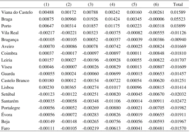
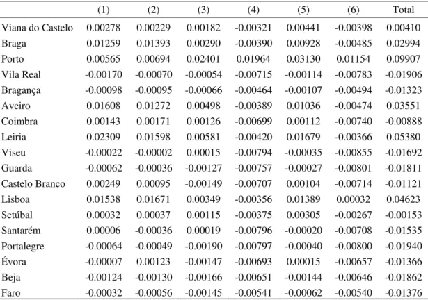
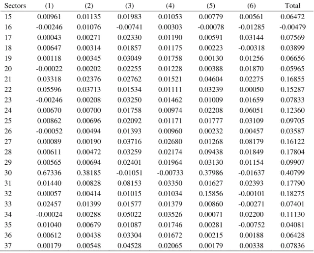
To illustrate the methodology Tables 1 and 2 show the results for two sectors disaggregating by county and Table 3 shows the results for a county disaggregating by sector. Given the vast number of counties analyzed, we present results only for those corresponding to the capital of the district (Continental Portugal is also divided into 18 districts). It is for the same reason of parsimony in presentation that Tables 1 and 2 show the results for only two sectors – the two with the highest values in terms of the total level of centrality (i.e., the sum of the several components of the centrality index) – namely wearing apparel, dressing and dyeing of fur (sector 18) and machinery and equipment n.e.c. (sector 29), and Table 3 shows the results for only the county with the highest (total) level of centrality in the country (Porto). All the remaining results are available upon request.
[Tables 1, 2, and 3 about here]
Let us analyze Table 1 for sector 18. The results show that the county with the highest centrality level for this sector is Braga and that only three counties (Viana do Castelo and Porto in addition to Braga), all located close to each other, reveal good conditions in terms of centrality in this sector, as the sum of the several components is negative for the remaining counties. Focusing on the contribution of each term of the centrality index with
6 Earlier studies used regional income but population or employment have also been considered.
7 There is a wide range of measures of intra-regional distances today. For a survey on this topic see Head
positive sign in Braga, by decreasing order, the proximity to suppliers in the region in which the sector is located (3) and in the nearby regions (4) stands out, followed by the economic dimension of the nearby regions (2) and of the region in which the sector is located (1); proximity to customers in the county (5) comes at the end of the ranking. Curiously, the qualitative results are very similar for the two other counties (Porto and Viana do Castelo), confirming the importance of proximity to suppliers and to similar activity as a relevant factor of location in the case of this sector.
As for the machinery and equipment n.e.c. sector (29), shown in Table 2, and considering the county with the highest level of centrality in this sector (Porto), the results highlight, by decreasing order, the internal proximity to buyers (5), the internal proximity to suppliers (3), the external proximity to suppliers (4) and buyers (6), and lastly, the external and internal economic components (2 and 1, respectively). Turning now to the 2nd county in terms of the total value of the index, Lisboa, we see that now standing out in descending order are the economic dimension of the nearby regions (2) and of the region itself (1), followed by internal proximity to buyers (5), which is in line with the particular attractiveness conditions of a region that includes the nation's capital.
Worth noting that in the privileged region for location of each sector, according to our index, we found intra-sectoral determinants of centrality in the clothing sector while in the machinery and equipment sector the most important factors all have an inter-sectoral type both backward and forward. These results are in accordance with the inherent characteristics of these sectors. Of course, different results can be observed for the same sector in different regions since the sectoral level chosen for this analysis is very aggregated; it is possible that within the same sector there are products more sensitive than others to a specific type of location factors.
Turning now to an analysis by county, Table 3 shows the results for the county with the highest value for the sum of the several components included in the centrality index (Porto).
proximity to buyers. This result is consistent with the fact that Porto is the second most prosperous region of the country.
Turning now to the 2nd component, in descending order we observe that in sector 30 the foreign economic component stands out and in sector 32 again an effect of an inter- industrial nature, in this case the internal component of proximity to suppliers.
4. Final remarks
This study contributes to the development of indicators of centrality and accessibility by taking into account a sectoral approach and determinant factors not yet considered in this empirical literature, namely the vertical linkages.
We are conscious that even the most sophisticated centrality indicators are at best surrogates for a vaguely perceived notion of “mass” of a region and “distance costs” (to use Keeble’s phrase). For instance, the absorptive capacity of the region where the sector locates also contributes to the centrality level of a sector, given for instance by support infrastructures, such as services and a network of schools. It may be that the way forward for this type of indicator lies in a more direct measurement of these effects.
Obviously, being a function of the actual distribution of the economic activity, the centrality level of the sectors may change in the future. However, some regions suffer a permanent penalty expressed in their disadvantage concerning their relative geographical position, with negative consequences, for instance, in terms of per capita income and human capital. This study provides some clues on ways to counteract this trend by promoting the centrality of some sectors, such as facilitating the establishment of upstream and downstream sectors in nearby areas, decreasing the physical accessibility to other regions, and/or favoring the geographical proximity of firms with similar economic activity.
References
Blainey, G. (1983), The tyranny of distance: How distance shaped Australia’s history,
Pan-Macmillan.
Brülhart, M. (2001), “Evolving Geographical Concentration of European Manufacturing Industries”, Welwirtschaftliches Archiv, 137(2), pp. 215-243.
Copus, A. (1999), “Peripherality index for the NUTS III regions of the European Union”, Report for the European Commission, ERDF/FEDER Study, 98, 00-27-130.
Duranton, G. and Overman, H. (2002), “Testing for localization using micro-geographic data”, The Review of Economic Studies, 72(4), pp.1077-1106.
Ellison, G. and Glaeser, E. (1997), “Geographic Concentration in U.S. Manufacturing Industries: A Dartboard Approach”, Journal of Political Economy, 105(5), pp. 889-927.
EU Commission (1998), “European Spatial Development Perspective”, Complete Draft, Glasgow.
Frost, M. and Spence, N. (1995), “The Rediscovery of Accessibility and Economic Potential: the Critical Issue of Self Potential”, Environment and Planning A, 27, pp.
1833-1848.
Head, K. and Meyer, T. (2002), “Illusory Border Effect: Distance Mismeasurement Inflates Estimates of Home Bias”, CEPII Working Paper, nº 2001-01.
Head, K. and Meyer, T. (2004), “The Empirics of Agglomeration and Trade” in
Handbook of Regional and Urban Economics, vol. 4, chap. 59, pp. 2609-2669, Ed:
Elsevier.
Keeble, D., Offord, J., and Walker, S. (1988), “Peripheral regions in a community of twelve Member States”, Report for the European Commission, Brussels.
Keeble, D., Owens, P., and Thompson, C. (1982), “Regional accessibility and economic potential in the European Community”, Regional Studies, 16(6), pp. 419-432.
Krugman, P. (1991), Geography and Trade, Cambridge: MIT Press.
Ottaviano, G. (2008), “Infrastructure and economic geography: An overview of theory and evidence”, European Investment Bank Papers, 13(2), pp. 8-35.
Schürmann, C. and Talaat, A. (2000), “Towards a European peripherality index”, Report for General Directorate XVI Regional Policy of the European Commission.
Spiekermann, K. and Neubauer, J. (2002), “European accessibility and peripherality: Concepts, models and indicators”, Nordregio Working Paper No. 2002:9, Nordregio, Stockholm.
Spiekermann, K. and Wegener, M. (2006), “Accessibility and Spatial Development in Europe”, Scienze Regionali, 5(2), pp. 15-46.
Table 1: Centrality by components in sector 18
(1) (2) (3) (4) (5) (6) Total
Viana do Castelo 0.00488 0.00172 0.00788 0.00242 0.00160 -0.00261 0.01589
Braga 0.00875 0.00960 0.01926 0.01424 0.00345 -0.00006 0.05523
Porto 0.00647 0.00314 0.01857 0.01175 0.00223 -0.00318 0.03899
Vila Real -0.00217 -0.00221 0.00323 -0.00375 -0.00082 -0.00555 -0.01126
Bragança -0.00105 -0.00105 0.00052 -0.00357 -0.00039 -0.00386 -0.00940
Aveiro -0.00070 -0.00086 0.00078 -0.00742 -0.00025 -0.00824 -0.01669
Coimbra 0.00037 -0.00017 -0.00097 -0.00897 0.00011 -0.00848 -0.01810
Leiria 0.00157 0.00027 -0.00196 -0.00928 0.00055 -0.00822 -0.01707
Viseu 0.00046 -0.00007 -0.00026 -0.00829 0.00013 -0.00807 -0.01609
Guarda -0.00055 0.00024 -0.00060 -0.00699 -0.00015 -0.00653 -0.01457
Castelo Branco 0.00180 0.00012 -0.00154 -0.00722 0.00054 -0.00620 -0.01251
Lisboa 0.00230 0.00365 -0.00274 -0.01017 0.00096 -0.00815 -0.01414
Setúbal -0.00123 -0.00122 -0.00251 -0.00820 -0.00045 -0.00670 -0.02032
Santarém -0.00035 -0.00058 -0.00348 -0.01106 -0.00014 -0.00911 -0.02472
Portalegre -0.00056 -0.00052 -0.00269 -0.00880 -0.00021 -0.00705 -0.01982
Évora -0.00056 -0.00072 -0.00283 -0.00826 -0.00019 -0.00655 -0.01911
Beja -0.00149 -0.00148 -0.00265 -0.00756 -0.00056 -0.00593 -0.01967
Table 2: Centrality by components in sector 29
(1) (2) (3) (4) (5) (6) Total
Viana do Castelo 0.00278 0.00229 0.00182 -0.00321 0.00441 -0.00398 0.00410
Braga 0.01259 0.01393 0.00290 -0.00390 0.00928 -0.00485 0.02994
Porto 0.00565 0.00694 0.02401 0.01964 0.03130 0.01154 0.09907
Vila Real -0.00170 -0.00070 -0.00054 -0.00715 -0.00114 -0.00783 -0.01906
Bragança -0.00098 -0.00095 -0.00066 -0.00464 -0.00107 -0.00494 -0.01323
Aveiro 0.01608 0.01272 0.00498 -0.00389 0.01036 -0.00474 0.03551
Coimbra 0.00143 0.00171 0.00126 -0.00699 0.00112 -0.00740 -0.00888
Leiria 0.02309 0.01598 0.00581 -0.00420 0.01679 -0.00366 0.05380
Viseu -0.00022 -0.00002 0.00015 -0.00794 -0.00035 -0.00855 -0.01692
Guarda -0.00062 -0.00036 -0.00127 -0.00757 -0.00027 -0.00801 -0.01811
Castelo Branco 0.00249 0.00095 -0.00149 -0.00707 0.00104 -0.00714 -0.01121
Lisboa 0.01538 0.01671 0.00349 -0.00356 0.01389 0.00032 0.04623
Setúbal 0.00032 0.00037 0.00115 -0.00375 0.00305 -0.00267 -0.00153
Santarém 0.00006 -0.00036 0.00019 -0.00796 -0.00020 -0.00708 -0.01535
Portalegre -0.00064 -0.00049 -0.00190 -0.00797 -0.00040 -0.00800 -0.01940
Évora -0.00007 0.00123 -0.00147 -0.00693 0.00015 -0.00657 -0.01366
Beja -0.00124 -0.00130 -0.00166 -0.00651 -0.00144 -0.00646 -0.01862
Table 3: Centrality by components in Porto
Sectors (1) (2) (3) (4) (5) (6) Total
15 0.00961 0.01135 0.01983 0.01053 0.00779 0.00561 0.06472
16 -0.00246 0.01076 -0.00741 0.00303 -0.00078 -0.01285 -0.00479
17 0.00043 0.00271 0.02330 0.01190 0.00591 0.03144 0.07569
18 0.00647 0.00314 0.01857 0.01175 0.00223 -0.00318 0.03899
19 0.00118 0.00345 0.03049 0.01758 0.00130 0.01256 0.06656
20 -0.00022 0.00202 0.02255 0.01228 0.00388 0.01870 0.05965
21 0.03318 0.02376 0.02762 0.01521 0.04604 0.02275 0.16855
22 0.05596 0.03713 0.01534 0.01111 0.03239 0.00050 0.15287
23 -0.00246 0.00208 0.03250 0.01462 0.01009 0.01659 0.07833
24 0.00670 0.00700 0.01758 0.00974 0.02208 0.06051 0.12360
25 0.00862 0.00696 0.02092 0.01171 0.01777 0.03109 0.09705
26 -0.00052 0.00494 0.01393 0.00960 0.00232 0.00457 0.03587
27 0.00089 0.00190 0.03716 0.02680 0.01268 0.08179 0.16122
28 0.00611 0.00472 0.03259 0.02174 0.09438 0.01849 0.17804
29 0.00565 0.00694 0.02401 0.01964 0.03130 0.01154 0.09907
30 0.67336 0.38185 -0.01051 -0.00733 0.37986 -0.01637 0.40799
31 0.01440 0.00828 0.08153 0.03350 0.01627 0.02393 0.17790
32 0.00057 0.00414 0.01015 0.01034 0.15856 -0.00101 0.18275
33 0.02457 0.01399 0.01577 0.01379 0.00860 -0.00271 0.07401
34 -0.00024 0.00288 0.05022 0.03526 0.00071 0.02200 0.11130
35 0.01040 0.00679 0.01087 0.01746 0.00281 -0.00752 0.04081
36 0.00612 0.00438 0.03304 0.01672 0.00215 0.00188 0.06428
37 0.00179 0.00548 0.04528 0.02065 0.00179 0.00338 0.07836
Annex
CAE rev. 2/ NACE nomenclature 15 – Manufacture of food products and beverages
16 – Manufacture of tobacco products 17 – Manufacture of textiles
18 – Manufacture of wearing apparel; dressing and dyeing of fur
19 – Tanning and dressing of leather; manufacture of luggage, handbags, saddlery, harness and footwear
20 – Manufacture of wood and of products of wood and cork, except furniture; manufacture of articles of straw and plaiting materials
21 – Manufacture of pulp, paper and paper products
22 – Publishing, printing and reproduction of recorded media 23 – Manufacture of coke, refined petroleum and nuclear fuel 24 – Manufacture of chemicals and chemical products
25 – Manufacture of rubber and plastic products
26 – Manufacture of other non-metallic mineral products 27 – Manufacture of basic metals
28 – Manufacture of fabricated metal products, except machinery and equipment 29 – Manufacture of machinery and equipment n.e.c.
30 – Manufacture of office machinery and computers
31 – Manufacture of electrical machinery and apparatus n.e.c.
32 – Manufacture of radio, television and communication equipment and apparatus 33 – Manufacture of medical, precision and optical instruments, watches and clocks 34 – Manufacture of motor vehicles, trailers and semi-trailers