Braz. J. Phys. vol.38 número1

(1)

Atomic Hydrogen Under Strong Soft X-Ray Pulses

A. R. B. de Castro

IFGW, UNICAMP, 13083-970, Campinas, SP, Brazil, and LNLS, CP 6192, 13083-970, Campinas, SP, Brazil

Received on 24 December, 2007

We discuss theoretically the behavior of atomic Hydrogen under irradiation with strong light pulses in the soft X-ray spectral region. The method consists in the direct numerical solution of the time dependent Schr ¨odinger equation. We find ranges of (high) peak incident intensityI0, where 2-photon absorption becomes more probable

than 1-photon absorption. At very high intensity, the total ionization probability goes very close to 1 and then decreases asI0is further increased.

Keywords: Free-electron-laser; Multi-photon absorption; Hydrogen

I. INTRODUCTION

In a series of recent papers the effect on a Helium atom, of short intense pulses in the XUV spectral range, was discussed both theoretically and experimentally [1-5] with regard to n-photon absorption of light at _ω_ph_{= 13 eV. The theoretical}

model contemplated the direct numerical solution of the Time Dependent Schr¨odinger Equation (TDSE) in a basis of finite and rather small dimensionality. In spite of the fact that the experimental results were in good agreement with the theory, the theory was questioned [6-8].

In what concerns the theory, the points of dissention seem to be (a) The use of approximate Helium electron eigenstates, which were not all orthogonal; (b) The fact that the procedure had not been tested by applying it to a well-known, previously solved problem; (c) The relevance of going beyond the Elec-tric Dipole Moment Approximation (EDMA).

We have, therefore, applied the same procedure to the case of a Hydrogen atom, which had been discussed before using other methods. For Hydrogen, all energy eigenstates of the isolated atom are exactly known and orthogonal. All matrix elements of the interaction termsp_•AandA_•Afor general kphoton>0 can be calculated with arbitrary numerical

preci-sion, if not as closed analytical expressions, at least as fast converging series. Exact expressions for all matrix elements are given in the Appendices. For our purpose of numerical solution of the Time Dependent Schr¨odinger Equation, these matrix elements were calculated to 6 significant figures and carefully checked as to convergence of the series. Then, we can also cover the EDMA case for purposes of comparison, simply by settingkphoton=0 in the general expressions.

We find fair quantitative agreement with previously pub-lished theoretical results.

II. SCENARIO 1 FOR THE CALCULATION

We assume the following scenario for the experiments: a photo-electron detector counts electrons resulting from ion-ization of the Hydrogen atoms and going into a small solid angle ∆Ω around thez axis, which we choose to be paral-lel to the direction of the electric fieldE in the linearly po-larized light beam. The radiation field is supposed to be single-mode (strictly monochromatic) with_ω_ph_{= 27.21 eV}

(kphrB=0.00729,kphorthogonal toE=Ez).

We consider only a small number of low-lyingbound eigen-states and twounboundeigen-states|k1>|k2>with definite k-vector in thezdirection; the energy eigen-values are E1= 2_k2

1/2me and E2= 2k22/2me. We choosek1k2so that both

transitions (from ground state 1s intok1and fromk1intok2)

are 1-photon resonant. An energy level diagram is shown in Fig. 1.

1s

2s 2p-1 2p0 2p1

k2

k1

E=0 E=0

FIG. 1: Hydrogen atom energy levels (not to scale), showing all transitions possible, if exact matrix elements are considered. For the geometry considered here, however, the transitions 2s and 1s-2p_±1are forbidden.

We have therefore the parameter values in Table I:

The quantized radiant field is described in terms of its en-ergy eigenstates. Let us add here that there is no cogent reason not to usea fully quantized radiation field. In fact, it allows us to keep track very conveniently of the system states, is per-fectly sound mathematically, and . . . nature seems to be quan-tum, not classical.

We should comment on the normalization of the quasi-free (E >0) eigenstates of the Hydrogen atom. From the point of view of solving a system of coupled 1st _order

dif-ferential equations it is much more convenient to divide up the k space (labels of the unbound states) into finite cells of volume (∆3_k)=k2_{dkdΩ, define the new states} _|_k_>

discr= (∆3_k)−1/2

ξ∈∆(k)d3ξ|ξ >and use instead of the set{|k>} the denumerable ortho-normal set{|k>discr}. We are

inter-ested in small values of(∆3_k)_{, describing the energy}

resolu-tion and angular acceptance of the photo-electron detector. For small (∆3_k)_,_|_k_>

discr∼=(∆3k)1/2|k>; we can therefore

(2)

TABLE I: Parameter values for the calculation in Scenario 1

Energy (eV) Wavevector Other

Photon energy_ω_ph _27.21 _k_ph_r_B_=0.00729 _kph_•_z₌₀

E•z=E Ionization potential IPH 13.606

Excited quasi-free state E1

E1=ωph-IPH

13.606 k1rB=1.000 k1•z=k1

E2= 2ωph-IPH

40.818 k2rB=1.732 k2•z=k2

If we consider energy resolution ∆E, and angular accep-tance limited to a cone of small half-angleθm aboutk, then

∆(k) = (πθ2

m)k3(1/2∆E/E). Take∆E/E=0.1,θm=0.174 rad

[5]. Then (∆3_k

1)= 43.2x10−4rB−3and (∆3k2)= 224.5x10−4

r−_B3.

Details of the calculation have been given elsewhere [1]; in short, we go over to the interaction picture [9] and solve a linear system of 1st order differential equations numerically, using the Hairer and Wanner [10] code. Let H′be the interac-tion term in the Hamiltonian. In dimensionless form (atomic

units), the system of equations is

i∂/∂tCn(t) =

∑

m

exp(iωnmt)<n|H′′|m>Cm(t)

ωnm = (En− −Em)/(2Rydberg)

H′′ = H′/(2 Rydberg) (1)

Here H′′ has two contributions. The first connects field states differing by 1 photon, while the second connects field states differing by 2 photons:

H′′_p.A = (1/2m)(e/c)<f in_|2A_•p_|ini>/(2Rydberg) = = i(1.76610−12_erg−1/2_sec1/2_cm√_I₎_<_{f in}_|_exp_(ik

ph•r)∂/∂z|ini> H_A.A′′ = (1/2m)(e/c)2<f in_|A_•A_|ini>/(2Rydberg) =

= (1.56110−24erg−1seccm2I)<f in_|exp(2ikph•r)|ini> (2)

whereIis the intensity (peak power density/unit area) in units of erg sec−1_cm−2_.

We assumed a smooth bell-shaped envelope for the laser pulse intensity, with peak power densityI0:

I(t) = I0sin2[3πt/2T] if 0<t<T/3 = I0 if T/3<t<2T/3 = I0sin2[3π(T−t)/2T] if 2T/3<t<T (3)

The index n in Cn(t) runs over a double set of 7 orbital

states (1s, 2s, 2p1, 2p0, 2p₋1,k1,k2)and 4 photon states N-j,

j=0,1,2,3 where N is the number of photons in the (single-mode) field, and j is the number of photons absorbed by the Hydrogen atom. So, there is a total of 21 complex functions Cn(t) to be determined. The system is solved under the initial

condition that the atom is in the ground state.

We have extensively checked the correctness of the numer-ical solutions in the context of quantum mechanics: it was, for instance verified that the system state norm is kept invariant to better than 1 part in 106, that the occupation probabilities do not depend on the phase of the initial condition, etc.

We have more recently performed additional tests. For in-stance, we can disable all transitions except one. In this way, we can simulate a two-level system, under resonant or non-resonant conditions, for absorption of one or two photons, un-der excitation with arbitrary time envelopes.

For either 1-photon absorption or 2-photon absorption, in the weak excitation limit, with fixed square or bell-shaped laser pulse envelope, under resonant conditions, we find that the occupation probability of the excited state depends on intensity linearly (1-photon absorption) or quadratically (2-photon absorption), as expected.

For either 1-photon absorption or 2-photon absorption, in the strong excitation limit, with long square pulse envelope, under resonant or non-resonant conditions, the occupation probability of the excited state, given by the numerical solu-tion of the TDSE, is found to depend on time, on the “detun-ing”ωnmand on field intensity just as predicted by the Rabi

equations [9].

We want to compare our results with the calculation by Nurhuda and Faisal [11], where the Electric Dipole Moment Approximation (EDMA) is used.

(3)

<f in_|exp(ikph•r)∂/∂z|ini>calculated according to the

gen-eral formulae in the Appendices (and settingkph=0). In the

EDMA,<f in_|exp(2ikph•r)|ini>=0.

TABLE II: Matrix elements∆(EDMA)for comparison with ref [11]. Transition Normalized dimensionless matrix

el-ement M

2s←1s 0

2p_±1 ←1s 0

2p0 ←1s -0.2793

k1z←1s -0.009346 i

k1z←2s -0.004445 i

k1z←2p_±1 0

k1z←2p0 0.0005552

k2z←1s -0.004746

k2z←2s 0.001921 i

k2z←2p_±1 0

k2z←2p0 0.00007007

k2z←k1z -0.00007503 i

The quantity needed for the numerical solution isγ= Cp.A

M √I0, where I0is the maximum intensity in units of 1012

W/cm2and Cp.A= 0.005584 i.

We used T = 93 atomic units of time and a field intensity range 1<I0<120 000 (x1012W/cm2), which spans the

re-gion up to and beyond the intensity considered in [11]. We focus on the occupation probabilities of the quasi-free orbital states k1k2for comparison with the results in Fig. 1 of ref

[11].

There are small differences in the normalization of the quasi-free states used here and in ref [6]; we think these are of minor significance, but are expected to change somewhat the numerical values.

Our discussion is centered on the radiant field intensity-dependence of the occupation probabilities after the excita-tion pulse is turned OFF, and on the time-dependence of the projections while the laser pulse is ON. The discussion of Nurhuda and Faisal [11] is centered on the electron-energy dependence of the ionization rate after the excitation pulse is finished, but at the single fixed radiation field intensity of 3.5x1016W/cm2.

Figure 2 shows the dependence on field intensity of the oc-cupation probability of the quasi-free statesk1andk2

imme-diately after the excitation pulse is finished.

At lower field intensity, the probability grows linearly with intensity, as expected for a 1-photon absorption process. The matrix elements for transitions from 1s intok1ork2have

al-most the same values, but the transition intok1is resonant,

while the transition intok2is not. The large detuning causes

the projection of the system state onk2to oscillate during the

excitation pulse, and the net transfer of population intok2is

very small.

At large field intensity, we witness strong non-linear and non-monotonic behavior of the probabilities P(k1)P(k2), as

found before [1]. There are narrow ranges of field intensities

FIG. 2: Probability of occupation for the atomic Hydrogen quasi-free statesk1andk2, immediately after completion of the light pulse. The

horizontal axis covers the range 1012up to 1017W/cm2. The light pulse is bell-shaped, with total duration of 93 atomic units of time and photon energyEph=27.21 eV. The full lines are the result of a

calculation in the Electric Dipole Moment Approximation. The full diamonds are the result of a calculation with exact matrix elements for both termsp_•AandA_•Aof the interaction.

(for instance, 3.0 to 4.0x1016_W/cm2_{) where the}_k

1

popula-tion P(k1) changes very rapidly, and goes successively thru

values much larger and much smaller than thek2population

P(k2). Nurhuda and Faisal find P(k1)/P(k2)∼10 at 3.5x1016

W/cm2 ), while in the present calculation, this happens at 3.0x1016 W/cm2. We attribute the difference to distinct cri-teria for normalization of the quasi-free states; while we nor-malized to the acceptance∆3_k_{of a typical electron analyzer}

placed along the direction of the radiant electric field vector

E_{, ref [6] does not specify the normalization of the states or}

the experimental arrangement.

Figure 3 shows the time development of the system state projections on the statek1. Let us observe that while the

ra-diant field is ON, we cannot speak of “electron state” because the electron is tightly coupled to the radiation field. However, the system state can still be written as a superposition of eigen-states from the isolated atom and the free radiation field, and we can follow the evolution of the projections. At lower field intensities, the projection onk1grows smooth and

monotoni-cally, as expected from elementary perturbation theory. How-ever, a complicated non-monotonic behavior is evident at high field intensity.

Regarding this complex behavior, let us observe that all two-level systems under harmonic steady-state excitation are exactly described by the Rabi equations [9]. These equations predict non-linear non-monotonic dependence of the popula-tions on field intensity. Here, on the other hand, we are dis-cussing a n-level(n>2)system excited by very short bell-shaped pulses, not a steady-state excitation. Furthermore, here the pulse length and the Rabi period for the transitions are comparable, and we expect a complicated interplay of these various effects.

(4)

FIG. 3: Time-dependence of the system-state projection on the elec-tron quasi-free statek1, at low incident intensity and at high incident intensity. In the former case we see a smooth monotonic increase of the projection, while in the latter case, a complicated non-monotonic evolution. At low intensity, the Rabi period is much longer than the pulse length. At high intensity, the pulse length and Rabi period have values in the same order-of-magnitude.

result of the exact calculation for the matrix elements ofp_•A andA_•A, setting kph=0.00729. It is clear from Fig. 2 that in

Hydrogen these corrections are significant only for the highest intensities (I0∼1016W/cm2)and affect mostly the

probabil-ity of occupation of the quasi-free state k₂, which requires 2-photon absorption in order to be populated.

Let us also observe that the deep minima shown in Fig. 2 are not believed to be experimentally observable, in so far as the experimental apparatus will collect not only photo-electrons going into the sharply definedk1(ork2)state, but also going

into neighboring quasi-free states, within some energy accep-tance. In the next section we address this question.

It is seen that our procedure, when applied to atomic Hydro-gen, under the conditions considered by Nurhuda and Faisal [11], reproduces their result regarding the ratio of probabili-ties for 1-photon and 2-photon absorption, except for a small shift (15%) in the value of the radiant field intensity. On the other hand, our calculation shows that the probabilities are changing very rapidly and by several orders of magnitude in this region of field intensities. A more detailed comparison would need more complete information about the normaliza-tion of the quasi-free electron states in [11], which has not been given.

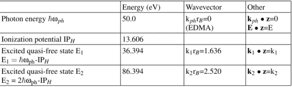
III. SCENARIO 2 FOR THE CALCULATION

Here we would like to compare our results with those of Bauer Plucinski Piraux Potvliege Gajda and Krzywinski [12]. They also used EDMA, with different pulse profile and inten-sity range.

We have here the parameter values given in Table III: The normalization constants are now (∆3_k

1)1/2 = 0.1375

and (∆3_k

2)1/2= 0.2629.

The pulse length here is T=103 atomic units while the pulse profile is

I(t) =I0sin2(πt/T) for 0<t<T, (4)

The intensity independent dimensionless matrix elements M are given in Table IV below.

Tables II and IV show that the matrix elements M change little on going from_ω_{= 27.21 eV to}_ω_{= 50 eV. However,}

for given M and_{ω, the transition rates are strongly affected}

by the resonant or non-resonant character of the process. So, we simulate the effect of adjoining quasi-free levels by repeat-ing the calculation with the same matrix elements M but intro-ducing energy displacementsδE in the quantitiesωnm. Then

we average over the group of adjoining quasi-free states. For each value of I0, we used groups of 5 quasi-free states, with

(δE1,δE2)= (0,0), (ε,0), (-ε,0), (0,ε), (0,-ε)andε= 2 eV, a

value which is consistent with the normalization of the quasi-free states.

FIG. 4: Probability of occupation for a group of 5 atomic Hydrogen quasi-free statesk1andk2, separated byδE=0,±2 eV, immediately after completion of the light pulse. The horizontal axis covers the range 1012up to 2.5 1019W/cm2.

The light pulse is bell-shaped (sin2), with total duration of 103 atomic units of time and photon energyEph=50 eV. The full lines are

the result of a calculation in the Electric Dipole Moment Approxi-mation. Notice the sudden increase in the population ofk2at about 2.5 1018_W/cm2_{, and the slopes 1 2 in the log-log plot, characteristic}

of 1-photon and 2-photon absorption at low intensity.

Figure 4 shows our results for the average occupation of each group (centered on k1 and k2, respectively). In our

model with a finite number of accessible orbital states, and for the experimental scenario described above, the total ion-ization probability per atom per incident pulse is the sum of the probabilities for going into the groupsk1andk2.

The figure shows that at low intensities, the population in groupk1(transition assisted by 1-photon absorption) is orders

of magnitude larger than in groupk2 (transition assisted by

(5)

TABLE III: Parameter values for the calculation in Scenario 2.

Energy (eV) Wavevector Other

Photon energy_ω_ph _50.0 _k_ph_r_B₌₀

(EDMA)

kph•z=0 E•z=E Ionization potential IPH 13.606

E1=ωph-IPH

36.394 k1rB=1.636 k1•z=k1

E2= 2ωph-IPH

86.394 k2rB=2.520 k2•z=k2

TABLE IV: Matrix elements∆ (EDMA)for comparison with ref [12].

Transition Normalized dimensionless matrix el-ement M

2s←1s 0

2p_±1 ←1s 0

2p0 ←1s -0.2793

k1z←1s -0.009864 i

k1z←2s -0.004045 i

k1z←2p_±1 0

k1z←2p0 0.0001699

k2z←1s -0.007276

k2z←2s 0.002761 i

k2z←2p_±1 0

k2z←2p0 0.00003754

k2z←k1z -0.001736 i

The figure also shows that at high intensities (above about 1016 W/cm2)the behavior is non-monotonic. At about 1018 W/cm2the population of thek2group shoots suddenly up and

exceeds the population of thek1group by roughly a factor of

10. The two populations then go down slowly as the incident field intensity is further increased.

It is not so easy to compare these results with ref [12] be-cause it is not clear what the authors mean by “ionization rate [a.u.]” in their figure 3, where the maximum value is∼0.07 at I0= 4x1017W/cm2, or “total ionization yield” in their

fig-ure 4, where a very broad maximum value∼0.95 is found at 2x1017_W/cm2_<_I

0<2x1018W/cm2. Our data gives a

max-imum ionization probability per atom per pulse_∼0.54 at I0=

2.5x1018W/cm2.

Figures 5 and 6 in ref [12] give also photo-electron spec-tra at incident intensities I0 = 2.5x1018 W/cm2 and I0 =

2.5x1019 W/cm2, both within the range of the present calcu-lation. There is clear disagreement between the results at I0=

2.5x1019W/cm2, since our calculation (see our figure 4) pre-dicts a 2-photon peak larger than the 1-photon peak, while ref [12] predicts a 1-photon peak larger than the 2-photon peak. Regarding the spectra at I0= 2.5x1018W/cm2, the

compari-son is inconclusive, because our occupation probabilities are changing very fast at precisely this field intensity. The posi-tion (along the intensity axis) of the cross-over is expected to

depend on the normalization of our quasi-free states, as ex-plained before.

There are other differences in the calculations, which may or may not have a bearing on these comparisons. We used exact Coulomb wave-functions with definitekfor the quasi-free states, which are an infinite sum of spherical waves. A large number of such waves was needed to reach convergence with 6 significant figures. The authors of ref [12], on the other hand, used the semi-classical approximation to set up the TDSE and solved it on a basis of Sturmian functions, which are not eigen-functions of the isolated hydrogen atom. Also, we explicitly address a situation where the photo-electron de-tector, although placed in the preferential direction for photo-ionization, collects electrons only on a restricted solid angle.

IV. DISCUSSION AND CONCLUSION

The non-monotonic dependence on incident light inten-sity, of occupation probabilities for quasi-free electron states involving absorption of 1, 2, . . . photons, found in the He-lium calculation [1] is evident also in the present calculation. Here, however, only exact eigen-states were used; the non-monotonic behavior just mentioned cannot therefore be asso-ciated with faulty approximate eigen-states, as has been sug-gested in the case of Helium [6,7].

For Hydrogen, and for the radiant field intensity range con-sidered in ref [11], the EDMA seems quite adequate. This shows also that the non-monotonic behavior of the probabil-ities for 1-photon and 2-photon absorption (at least in Hy-drogen) do not depend exclusively on the exact forms of the p_• AandA _•A interaction terms. Upon consideration of the detailed time-dependence of the system-state projections it is clear that, for sufficiently short and powerful laser pulses, many quasi-free states will be populated whether or not the transition is resonant. Physically, this is completely consistent with the fact that a sufficiently short pulse cannot be strictly monochromatic.

Regarding the calculation of the matrix elements, where misleading symmetry arguments are often invoked to claim they should vanish, let us observe the following:

1) The matrix element ofA_• Ais non-vanishing in gen-eral, although it is zero whenkphoton=0 and the initial and final

states are orthogonal. Therefore, even for smallkphoton, it may

(6)

very high peak power density applications. This is in sharp contrast to the opinion of our critics [6-8].

2) If the matrix element of p.A has a finite value at kphoton=0, the next correction is, for initial and final states

of usual interest and current FEL wavelengths, comparatively very small. Here, it seems quite safe to use the EDMA (kphoton=0) without further ado, as most text-books teach, and

as our critics [6-8] hold to be the correct way to deal with matter-light calculations in a regime similar to the one we con-templated in [1].

Regarding comparison with previous theoretical results in the literature, we find quantitative agreement within 15% for the relative intensities of photo-electron peaks at intensities close to 3.5x1016 _W/cm2_{, resulting from 1 and 2 photon}

ab-sorption as calculated by Nurhuda and Faisal [11]. We find qualitative agreement with ref [12] in so far as both calcula-tions predict almost complete (95% in ref [12], 54% in our

calculation) ionization at intensities close to 2.5x1018W/cm2, and a “stabilization” effect (reduction in the ionization yield as the intensity is even further increased). We disagree on the relative intensities of the photo-electron peaks at 2.5x1019 W/cm2. As far as the author knows, there are not yet experi-mental results to check such calculations.

Acknowledgements

ARBC acknowledges financial help from FAPESP for visits to TU Berlin and HASYLAB am DESY, where part of these calculations was done. He also acknowledges many fruit-ful discussions with Thomas M¨oller (TU Berlin) which were essential to weed out programming mistakes and clarify the physical meaning of the results. He also thanks the two insti-tutions for making his stay in Germany very pleasant indeed.

Appendix 1: definitions and useful formulae

Theexact_{normalized energy eigenstates for Hydrogen are (using spherical coordinates}_r_{θϕ, with r given in units of}_r_B_and_k

in units ofr_B−1;1F1are confluent hypergeometric functions)

(eq. (1.1);bound stateswith definitelm)

|nlm>=fnl(r)Ylm(θϕ)

fnl(r) =Nnl(2r/n)lexp(−r/n)1F1(1+l−n,2+2l,2r/n)

Nnl=2[n2(2l+1)!]−1[(n+l)!/(n−l−1)!]1/2

(eq. (1.2);unbound Coulomb states with definitelm)

|k,lm> = C(k,l)(2ikr)lexp(−ikr)

1F1(1+l+i/k,2+2l,2ikr)Ylm(θϕ) C(k,0) = (2/√k)[1−exp(−2π/k)]−1/2

C(k,l) = (2/√k)[1−exp(−2π/k)]−1/2 [l!/(1+2l)!]

_∏

s=1,l

[1+ (ks)−2]1/2 (l>0)

The unbound Coulomb states with definitelmare formally obtained from the bound states replacing 1/nwithikandN_nlwith C(k,l).

(eq. (1.3);unbound Coulomb stateswith definitek)

|k>=

_∑

_lmYlm(ek)∗ |k,lm>

The energy eigenvalues areEn=−E0/n2, withE0=e2/rBfor the bound states andE(k) = (∇k)2/2mefor the unbound states.

They are degenerate with respect to the orbital angular momentum quantum numberslm. The radial function of the unbound states,{(2kr)l_exp₍₋_ikr)

1F1(1+l+i/k,2+2l,2ikr)}(with noifactor in(2kr)l), has been

shown to be real [13].

The following developments will be useful:

(7)

jS(u) = [uS/(2S+1)!!]exp(−iu)1F1(1+S,2+2S,2iu) (1.5a) jS(u) =

∑

∞ q=0b

(S) q u2q+S

with

b(qS)=2S(−1)q(q+S)!/[(1+2q+2S)!q!] (1.5b) jS(u) =

∑

S+1 q=0u−

q_[A(S)

q exp(iu) +B(qS)exp(−iu)] (1.5c)

TheA(qS)B(qS)follow from the recursion relations of the spherical Bessel functions.

We adopt the following convention for the phase of the spherical harmonic functionsYlm: Ylm(θϕ) =WlmPl|m|(cosθ)exp(imϕ)

Wlm= (−1)(m+|m|)/2[(2l+1)/4π]1/2[(l− |m|)!/(l+|m|)!]1/2 (1.6)

The following identities for hypergeometric functions [15] were extensively used in the calculation of matrix elements:

1F1(−n,c,z) = n

∑

v=0

[(−n)v/(cvv!)]zv ifn≥0 is an integer (1.7a)

1F1(a,c,z) =Γ(c)Γ(a)−1Γ(c−a)−1

1

0

dteztta−1(1−t)c−a−1 _if _Re(c)_>_Re(a)_>₀ ₍_1.7b₎

2F1(a,b,c,z) = b−c

∑

v=0

[av(c−b)v/(cvv!)](−z)v(1−z)−a−v if b−c≥0 is an integer (1.7c)

2F1(a,b,c,z) =Γ(c)Γ(c−b−a)Γ(c−b)−1Γ(c−a)−1 c−b−1

∑

v=0

[bv(b−c+1)v/(v!(b−c+a+1)v)]z−b−v(z−1)v. . .

+(−1)c−b−a_Γ_(c)_Γ_(b₋_c+_a)_Γ_(b)−1_Γ_(a)−1b

_∑

−1 v=0

[(c−b)v(1−b)v/(v!(c−b−a+1)v)]z−b−c(z−1)v+c−b−a

ifc₋b_≥1 andb_≥1 are integers (1.7d)

2F1(a,b,c,z) =Γ(c)Γ(b)−1Γ(c−b)−1

1

0

dttb−1(1−t)c−b−1(1−zt)−a if |z_|<1, and also Re(b)>0, Re(c−b)>0 (1.7e)

∞

0

drrMe−₁ζrF1(a,c,κr) = [Γ(M+1)/ζM+1]2F1(a,M+1,c,κ/ζ) if Re(ζ)>0 and M>−1 (1.7f)

∞

0

drrM−1e−₁ζrF1(a,M,kr)1F1(a′,M,k′r) =Γ(M)ζa+a ′₋_M

(ζ−k)−a₍_ζ₋_k′₎−a′

2 F1(a,a′,M,u)

where u=kk′/(ζ−k)(ζ−k′) and we require Re(ζ)>0 and M>0 (1.7g)

∞

0

drrM−1+se₁−ζrF1(a,M,kr)1F1(a′,M,k′r) = (−∂/∂ζ)s{Γ(M)ζa+a ′₋_M

(ζ−k)−a₍_ζ₋_k′₎−a′

2 F1(a,a′,M,u)} (1.7h)

Appendix 2: matrix elements of A

_•

p

Following standard procedures [13,14], we get the following exact matrix elements for general transitions betweenbound states(we choose thezaxis parallel to the radiation electric fieldE), induced by the term linear inA(r) (A(r) is the spatially dependent part of the vector potential operator for the radiation field) in the electron-radiation interaction:

<νλµ_|exp(ikph•r)∂/∂z|nlm>= ∞

∑

S=0 S

∑

σ=−S

{Fang(+)Frad(+)+F (−)

angFrad(−)} (2.1)

Fang(+)=4πiSYSσ∗(εph)

dΩY_λµ∗YSσYl+1m[(l+1−m)(l+1+m)/(2l+1)(2l+3)]1/2 l≥0

(8)

=4πiSYSσ∗(εph)

dΩYλµ∗YSσYl−1m[(l−m)(l+m)/(2l+1)(2l−1)]1/2 if l>0 (2.2)

The angular integrals vanish for most choices of the parameters in the spherical harmonic functions, see (eq. 2.3) below. The “3Y” factor

dΩYl1m1∗Yl2m2Yl3m3vanishes exactly, unless

m1+m2+m3=0 (2.3a)

l1+l2+l3=even integer (2.3b)

l1,l2,l3 non-negative integers satisfying the “triangular inequalities” |l1−l2| ≤l3≤l1+l2

and |l2−l3| ≤l1≤l2+l3

and|l3−l1| ≤l2≤l3+l1

and if any one of the three numbers is zero, the other two must be equal.

(2.3c) Such conditions restrict the sums over angular momentum quantum numbers very strongly. In addition, it may also happen that the Y’s in the prefactors independently vanish for certain choices of the directions of incident field polarization and propagation vectorkph=kphεph.

In the sum in (eq. 6) it is obvious that contributions withS>λ+l+1 have null angular coefficients. For the geometry of our helium experiments in the DESY FEL Phase 1, thezaxis was chosen parallel to the radiant electric field, then, due to transversality, cosθ=0 and there are even less non-trivial choices ofλSlfor eitherFang(+)orFang(−).

The radial integrals are

F_rad(−) =

∞

0

r2dr jS(kphr)fνλ(r)[∂fnl/∂r+ [(1+l)/r]fnl]

= N_νλNnln−l−1ν−λ

−

∞

0

r2dr jS(kphr)(2r)λ+lexp[−r(1/n+1/ν)]1F1[1+λ−ν; 2+2λ; 2r/ν]1F1[1+l−n; 2+2l; 2r/n]

. . . + n(1+2l)

∞

0

. . . + [(1+l−n)/(1+l)]

∞

0

F_rad(+) =

∞

0

r2dr jS(kphr)fνλ(r)[∂fnl/∂r−[l/r]fnl]

= N_νλNnln−l−1ν−λ

−

∞

0

. . . + [(1+l−n)/(1+l)]

∞

0

(2.4) All integrals inFradcan be expressed exactly in terms of standard hypergeometric functions2F1:

F_rad(+) = (− −1/n)NνλNnl(kph)S[(2S+1)!!]−1

∑

( ν₋λ₋1) u=0

∑

(n₋l₋1) v=0 (2/ν)

u+λ₍_2/_n)v+l_{. . .}

. . . [(1+λ−ν)u/[u!(2+2λ)u]][(1+l−n)v/[v!(2+2l)v]]Γ(M+1)ζ−2M−1F1(1+S;M+1; 2+2S; 2ikph/ζ). . .

. . . + [(1+l−n)/(n+nl)]NνλNnl(kph)S[(2S+1)!!]−1

∑

(ν−λ−1) u=0

∑

(n−l−2) v=0 (2/ν)

u+λ₍_2/_n)v+l_{. . .}

. . . [(1+λ₋ν)u/[u!(2+2λ)u]][(2+l−n)v/[v!(3+2l)v]]Γ(M+1)ζ−2M−1F1(1+S;M+1; 2+2S; 2ikph/ζ) M _≡ 2+λ+l+S+u+v

ζ ≡ 1/ν+1/n+ikph

F_rad(−) = (− −1/n)NνλNnl(kph)S[(2S+1)!!]−1

∑

(ν−λ−1) u=0

∑

(n−l−1) v=0 (2/ν)

u+λ₍_2/_n)v+l_{. . .}

. . . [(1+λ−ν)u/[u!(2+2λ)u]][(1+l−n)v/[v!(2+2l)v]]Γ(M+1)ζ−₂M−1F1(1+S;M+1; 2+2S; 2ikph/ζ). . .

. . . + (1+2l)NνλNnl(kph)S[(2S+1)!!]−1

∑

(ν−λ−1) u=0

∑

(n−l−1) v=0 (2/ν)

u+λ₍_2/_n)v+l_{. . .}

. . . [(1+λ₋ν)u/[u!(2+2λ)u]][(1+l−n)v/[v!(2+2l)v]]Γ(M)ζ−2MF1(1+S;M; 2+2S; 2ikph/ζ). . .

. . . + [(1+l−n)/(n+nl)]NνλNnl(kph)S[(2S+1)!!]−1

∑

(ν−λ−1) u=0

∑

(n−l−2) v=0 (2/ν)

u+λ₍_2/_n)v+l_{. . .}

(9)

For the simplest case of interestν=2,λ=1,n=1,l=0 only the termsS=0,2 survive. They reduce to the elementary result [−(2/3)4√₂_]_{in the electric dipole approximation}_k

ph=0.

Similarly, for transitions from aboundinto aquasi-freestate, we get

<k_e|exp(ikph•r)∂/∂z|nlm>= ∞

∑

λ=0 λ

∑

µ=−λ ∞

∑

S=0 S

∑

σ=−S

Gang(+)G(+)_rad +Gang(−)G(_rad−)

(2.6)

G(+)ang = 4π(−1)λiSYλµ(εke)YSσ∗(εph)

dΩYλµ∗YSσYl+1m[(l+1−m)(l+1+m)/(2l+1)(2l+3)]1/2 l≥0 G(ang−) = 0 if l=0

= 4π(−1)λiSY_λ_µ(εke)YSσ∗(εph)

dΩY_λ_µ_∗YSσYl₋1m[(l−m)(l+m)/(2l+1)(2l−1)]1/2 if l>0

(2.7) (εkealongz,εphorthogonal toz).

For the radial integrals, case bound-free transitions,

G(+)_rad =

∞

0

r2dr(2iker)λexp[−iker]1F1[1+λ+i/ke; 2+2λ; 2iker]jS(kphr)[∂fnl/∂r−[l/r]fnl] = C(ke,λ)Nnln−l−1

−int₀∞r2dr jS(kphr)(2ker)λ(2r)lexp[−r(1/n+ike)] 1F1[1+λ+i/ke; 2+2λ; 2iker]1F1[1+l−n; 2+2l; 2r/n]

. . . + [(1+l₋n)/(1+l)]

∞

0

r2dr jS(kphr)(2ker)λ(2r)lexp[−r(1/n+ike)]

1F1[1+λ+i/ke; 2+2λ; 2iker]1F1[2+l−n; 3+2l; 2r/n]

G(_rad−) =

∞

0

r2dr(2iker)λexp[−iker]

1F1[1+λ+i/ke; 2+2λ; 2iker]jS(kphr)[∂fnl/∂r+ [(1+l)/r]fnl] = C(ke,λ)Nnln−l−1

−

∞

0

r2dr jS(kphr)(2ker)λ(2r)lexp[−r(1/n+ike)] 1F1[1+λ+i/ke; 2+2λ; 2iker]1F1[1+l−n; 2+2l; 2r/n]

. . . + n(1+2l)

∞

0

r1dr jS(kphr)(2ker)λ(2r)lexp[−r(1/n+ike)] 1F1[1+λ+i/ke; 2+2λ; 2iker]1F1[1+l−n; 2+2l; 2r/n]

. . . + [(1+l₋n)/(1+l)]

∞

0

r2dr jS(kphr)(2ker)λ(2r)lexp[−r(1/n+ike)]

1F1[1+λ+i/ke; 2+2λ; 2iker]1F1[2+l−n; 3+2l; 2r/n]

(2.8) These integrals no longer have exact analytic expressions in terms of elementary special functions. They can, however, be written in terms of some integrals over the interval (0,1) which are easy to calculate numerically, and which reduce to some2F1in the

special casesα=0,q=0, orα₋M₋1−q=0, orx=0 ory=0:

G(+)_rad = C(ke,λ)Nnl(2ike)λ(kph)S(2/n)l[(2S+1)!!]−1. . .

. . . (−1/n)

_∑

n_v₌−l₀−1[(1+l₋n)v/(v!(2+2l)v)](2/n)v Γ(1+M). . .

. . .

_∑

1_q+₌M₀−Λ[(Λ−M₋1)q(α)q/(q!(Λ)q)](−2ike)q(ζ−2ike)−α−qζα−M−1ϒ(S)

1

0

dttS(1−t)S(1−xt)α−M−1−q(1−yt)−α + (1+l−n)(n+nl)−1

_∑

_vn₌−₀l−2[(2+l₋n)v/(v!(3+2l)v)](2/n)vΓ(1+M). . .

. . .

_∑

1

0

dttS(1−t)S₍₁₋_xt)α−M−1−q₍₁₋_yt₎−α

(10)

with

ϒ(S) =Γ(2+2S)[Γ(1+S)]−2

M=2+λ+l+S+v(notice that this depends onv, a summation index) [Λ=2+2λ]

α=1+λ+i/ke

ζ=1/n+ike+ikph x=2ikph/ζ y=2ikph/(ζ−2ike)

G(_rad−) = C(ke,λ)Nnl(2ike)λ(kph)S(2/n)l[(2S+1)!!]−1. . .

. . . (−1/n)

_∑

_vn₌−l₀−1[(1+l₋n)v/(v!(2+2l)v)](2/n)vΓ(1+M)(ζ−2ike)−α. . .

. . .

_∑

1

0

dttS(1−t)S₍₁₋_xt₎α−M−1−q₍₁₋_yt)−α

+ (1+2l)

_∑

_vn₌−₀l−1[(1+l₋n)v/(v!(2+2l)v)](2/n)vΓ(M)(ζ−2ike)−α. . .

. . .

_∑

M_q₌−₀Λ[(Λ₋M)q(α)q/(q!(Λ)q)](−2ike)q(ζ−2ike)−α−qζα−Mϒ(S)

1

0

dttS(1−t)S(1−xt)α−M−q(1−yt)−α + (1+l−n)(n+nl)−1

_∑

n_v₌−₀l−2[(2+l₋n)v/(v!(3+2l)v)](2/n)v Γ(1+M)(ζ−2ike)−α. . .

. . .

_∑

1

0

dttS(1−t)S₍₁₋_xt)α−M−1−q₍₁₋_yt₎−α

(2.10)

Finally, we discuss transitions intounboundk’fromunboundkstates.

Let us start by saying that if one uses plane waves exp(−ik_•r)to describe the unbound electron states, 1-photon absorption is strictly forbidden due to conservation of energy and linear momentum. In fact, the matrix element of p.A is in this case proportional toδ(k2-k1+kphoton). Typical values for experiments at the DESY FEL Phase 1 would bekphoton= 0.00035,k1=

0.35,k2= 1.05, all in units ofr_Bohr−1 . It is clear there is no way to make the argument of theδ-function vanish.

If, however, we consider exact Coulomb states (unbound electron in the presence of a positive ion, eq. 1.2 or eq. 1.3) we find a rather large value for the matrix element, comparable to values for 1-photon absorption in the transitions (ground state)? (excited bound state).

The exact matrix element can be written as an infinite series only, but for parameter values of current interest, the series converges very rapidly. The result, assuming the radiant fieldEis parallel toz, and using the definitions below is,

α = 1+l+i/k α′ = 1+l′+i/k′

Λ = 2+2l Λ′ = 2+2l′

ε = k/k ε′ = k′/k′ εph = kph/kph

(2.11)

<k’_|exp(ikph•r)∂/∂z|k> =

∑

lml

∑

′m′

∑

Sσ

Hang(+)(l′m′ε′,Sσεph,lmε)Hrad(+)(l′k′,Skph,lk). . .

. . . +

_∑

lml

∑

′m′

∑

Sσ

Hang(−)(l′m′ε′,Sσεph,lmε)Hrad(−)(l′k′,Skph,lk)

(11)

Hang(+)(l′m′ε′,Sσεph,lmε) = 4πiSYl′m′(ε′)Y∗Sσ(εph)Ylm∗(ε)[(l+1+m)(l+1−m)(2l+1)−1(2l+3)−1]1/2. . .

. . .

dΩθϕY∗l′m′(θϕ)YSσ(θϕ)Yl+1,m(θϕ) l≥0

Hang(−)(l′m′ε′,Sσεph,lmε) = 0 if l=0

= 4πiSY_l′m′(ε′)Y∗Sσ(εph)Ylm∗(ε)[(l+m)(l−m)(2l+1)−1(2l−1)−1]1/2. . .

. . .

dΩθϕYl′m′∗(θϕ)YSσ(θϕ)Yl−1,m(θϕ) if l>0

(2.13)

H_rad(+)(l′k′,Skph,lk) = C(k,l)C(k′,l′)(2ik)l(2ik′)l ′

. . .

. . .(−ik)

∞

0

r2+l+l′drexp[−i(k+k′)r]jS(kphr)1F1(α′,Λ′,2ik′r)1F1(α,Λ,2ikr). . .

. . .+ [ik−(1+l)−1]

∞

0

r2+l+l′drexp[−i(k+k′)r]jS(kphr)1F1(α′,Λ′,2ik′r)1F1(α+1,Λ+1,2ikr)

H_rad(−)(l′k′,Skph,lk) = C(k,l)C(k′,l′)(2ik)l(2ik′)l ′

. . .

. . .(1+2l)

∞

0

r1+l+l′drexp[−i(k+k′)r]j_λ(kphr)1F1(α′,Λ′,2ik′r)1F1(α,Λ,2ikr). . .

. . .(−ik)

∞

0

r2+l+l′drexp[−i(k+k′)r]jλ(kphr)1F1(α′,Λ′,2ik′r)1F1(α,Λ,2ikr). . .

. . . + [ik−(1+l)−1_] ∞ 0

r2+l+l′drexp[−i(k+k′)r]j_λ(kphr)1F1(α′,Λ′,2ik′r)1F1(α+1,Λ+1,2ikr)

(2.14)

The expressions for transitions with bound or unbound initial or final states have all the same form, and can be obtained formally from each other by replacement of Nnl and 1/n occurring forbound states, with C(k,l)andik, occurring forunbound states. Here, however, the1F1do not, in general, reduce to polynomials, because the argumentsαα’ are not negative integers.

These integrals must be handled with care.

The radial integrals are all, generally speaking, non-vanishing. On the other hand, in the angular functions we have “3 Y” integrals which vanish for most values of the arguments, in particular forS>l+1+l′(inHang(+))and forS>l−1+l′(inHang(−)).

For the radial integrals corresponding tonon-zero angular integrals, we might use the spherical Bessel function expansion (eq. 1.5c) which is a finite sum of inverse powers(kphr)−q, 1≤q≤S+1. Notice that, given the restrictions 0≤S≤l+l′+1

(forH_rad(+)), 0≤S_≤l+l′₋1 (forH_rad(+))just mentioned, the integrand will never be singular at the origin. In addition, we use the integral representation (eq. 1.7b) for1F1(α,Λ,2ikr)plus (eq. 1.7f). We can also use the infinite power series representation,

(eq. 1.5b).

From a practical point of view, however, the development into exponentials is numerically inefficient, because the result depends on differences of large quantities which are almost the same. In addition, it is not easily applicable to the limit kph=0

because of the factors k−_phq, 1≤q_≤S+1. We have, however, calculated some of these integrals for purposes of checking. The calculations take about 10 times longer than using the power series expansion (eq. 1.5b) of the spherical Bessel function (discussed below) and precision is not as good. But the results agree to within 1 part in 105, and show that the general formulae are not in error.

(12)

H_rad(+) = C(k,l)C(k′,l′)(2ik)l(2ik′)l′

_∑

Qmax_q₌₀ k_ph2q+Sb(qS)

(−ik)Γ(M+1)Γ(Λ)Γ(α)−1_Γ₍_Λ₋_α₎−1 1 0

dttα−1(1−t)Λ−α−1₍_ζ₋₂_ikt)−M−1

2 F1(α′,M+1,Λ′,z). . . + [ik−(1+l)−1]Γ(M+1)Γ(Λ)Γ(α)−1Γ(Λ−α)−1

1

0

dttα−1(1−t)Λ−α−1(ζ−2ikt)₂−M−1F1(α′+1,M+1,Λ′+1,z)

H_rad(−) = C(k,l)C(k′,l′)(2ik)l(2ik′)l′

_∑

Qmax_q₌₀ k2q_ph+Sb(qS)

(1+2l)Γ(M)Γ(Λ)Γ(α)−1_Γ₍_Λ₋_α₎−1 1 0

dttα−1(1−t)Λ−α−1₍_ζ₋₂_ikt)−M

2 F1(α′,M,Λ′,z)

(−ik)Γ(M+1)Γ(Λ)Γ(α)−1Γ(Λ−α)−1

1

0

dttα−1(1−t)Λ−α−1(ζ−2ikt)₂−M−1F1(α′,M+1,Λ′,z). . .

+ [ik−(1+l)−1]Γ(M+1)Γ(Λ)Γ(α)−1Γ(Λ₋α)−1

1

0

dttα−1(1₋t)Λ−α−1(ζ₋2ikt)₂−M−1F1(α′+1,M+1,Λ′+1,z)

(2.15) where, now, we assumek<k′in order to avoid singular integrands, and define

M = 2+l+l′+2q+S ζ = ik+ik′

z = 2ik′/(ζ−2ikt)

Depending on the exponents, the integrand may result ill-conditioned at the end pointst=0 andt=1. Then we truncate the integration, i.e, we integrate in the intervalε<t<1−ε, withε∼10−7_.

Appendix 3: Matrix elements of

A

_•

A

Now we discuss the matrix elements<final_|exp(2ikph•r)|initial>, wherefinalandinitialcan be bound or unbound energy

eigenstates, withEf inal>Einitial.

Ifkph=0 they vanish identically because eigenstates with different energy are orthogonal. We are, of course, interested in the

general casekph>0.

For 2-photon bound-bound transitions we have <νλµ_|exp(2ikph•r)|nlm> =

drr2dΩf_νλ(r)Yλµ∗(θϕ)exp(2ikph•r)fnl(r)Ylm(θϕ)

=

_∑

Sσ

4πiSYSσ∗(εph)

dΩY_λ_µ_∗(θϕ)YSσ(θϕ)Ylm(θϕ)

drr2f_νλ(r)jS(2kphr)fnl(r)

=

_∑

Sσ

Iang(b−b)I_rad(b−b)

Iang(b−b) = 4πiSYSσ∗(εph)

I_rad(b−b) =

drr2f_νλ(r)jS(2kphr)fnl(r)

(3.1) The “3Y” angular integral has already been discussed. Using expansion (eq. 1.5a) for jS(u)and the definition (eq. 1.1) of the

bound state radial functions,

I_rad(b−b) = N_νλNnl(2/n)l(2/ν)λ[(2kph)S/(2S+1)!!]

drr2+l+λ+Sexp(−r/ν)1F1(1+λ−ν,2+2λ,2r/ν)

. . .

. . .exp(−2ikphr)1F1(1+S,2+2S,4ikphr)}{exp(−r/n)1F1(1+l−n,2+2l,2r/n)

(13)

(3.2) The1F1related to the bound states are always polynomials in r. Inserting the appropriate sums and then using the integral in

(eq. 1.7f), we get

I_rad(b−b) = N_νλNnl(2/n)l(2/ν)λ[(2kph)S/(2S+1)!!]. . .

. . .

ν−λ−1

∑

u=0 n−l−1

∑

v=0

[(2/ν)u₍₁₊_λ₋_ν₎

u/u!(2+2λ)u][(2/n)v(1+l−n)v/v!(2+2l)v]. . .

. . .Γ(M+1)ζ−M−1

2 F1(1+S,M+1,2+2S,4ikph/ζ) M = 2+l+λ+S+u+v

ζ = 1/n+1/ν+2ikph

(3.3) The possible values ofλSlare restricted to|λ−l_{| ≤}S_≤λ+lwithλ+S+l=even due to the angular integral.

Similarly, we have for a 2-photon bound-free transition

<k′_|exp(2ikph•r)|nlm> =

drr2dΩΨk′∗(rθϕ)exp(2ikph•r)fnl(r)Ylm(θϕ) =

_∑

λµ

Y_λ_µ(ε′)

_∑

Sσ

4πiSYSσ∗(εph)

drr2ψνλ(r)jS(2kphr)fnl(r)

=

_∑

λµ

∑

Sσ

Iang(b−b)I_rad(b−b)

Iang(b−free) = 4πiSYλµ(ε’)YSσ∗(εph)

I_rad(b−free) =

(3.4)

I_rad(b−free) = C(k′,λ)Nnl(2/n)l(2ik′)λ[(2kph)S/(2S+1)!!]

drr2+l+λ+Sexp(−r/n₋ik′r₋2ikphr). . .

. . .1F1(1+λ+i/k′,2+2λ,2ik′r)1F1(1+S,2+2S,4ikphr)1F1(1+l−n,2+2l,2r/n)

(3.5) The last1F1factor is still a polynomial in(2r/n)and we develop it:

I_rad(b−free) = C(k′,λ)Nnl(2/n)l(2ik′)λ[(2kph)S/(2S+1)!!] n₋l₋1

∑

v=0

[(2/n)v(1+l−n)v/v!(2+2l)v]. . .

. . .

drr2+l+λ+Sexp(−r/n₋ik′r₋2ikphr)1F1(1+λ+i/k′,2+2λ,2ik′r)1F1(1+S,2+2S,4ikphr)

(3.6) In some special cases, the remaining radial integral can be written as a closed analytical expression [13].

In general, the integral is calculated numerically. We replace one of the1F1factors with its integral representation and then

integrate in dr, to get

drr2+l+λ+S+vexp(−r/n₋ik′r₋2ikphr)1F1(1+λ+i/k′,2+2λ,2ik′r)1F1(1+S,2+2S,4ikphr) = = Γ(2+2S)Γ(1+S)−2_M_! 1

0

dttS(1−t)S₍_ζ₊₄_ik

pht)−2M−1F1(1+λ+i/k′,M+1,2+2λ,2ik′/(ζ+4ikpht)) M = 2+l+λ+S+v

ζ = 1/n+ik′+2ikph

(14)

<k′_|exp(2ikph•r)|k> =

drr2dΩΨ∗_k′(rθϕ)exp(2ikph•r)Ψk(rθϕ) =

_∑

λµ

Y_λ_µ(ε′)

_∑

Sσ

4πiSY_S∗_σ(εph)

∑

lm

Y_lm∗(ε). . .

. . .

dΩY_λ∗_µ(θϕ)YSσ(θϕ)Ylm(θϕ)

drr2ψνλ(r)jS(2kphr)ψnl(r) =

_∑

λµ

∑

Sσ

∑

lm

Iang(f−f)I_rad(f−f) ₍_3.8₎

Iang(free−free) = 4πiSYλµ(ε′)YS∗σ(εph)Ylm∗(ε)

dΩY_λ∗_µ(θϕ)YSσ(θϕ)Ylm(θϕ)

I_rad(free−free) =

= C(k′,λ)C(k,l)(2ik′)λ(2ik)l

drr2+l+λ+Sexp[−i(k+k′)r]jS(2kphr). . .

. . .1F1(1+λ+i/k′,2+2λ,2ik′r)1F1(1+l+ik,2+2l,2ikr) (3.9)

Here again we must develop the spherical Bessel function using either an infinite power series (eq. 1.5b) or a finite sum of exponentials, (eq. 1.5c). In either case the integral is of the type in (eq. 3.7).

We have used both approaches, as a means of internal checking.

[1] A. R. B. de Castro, T. Laarmann, J. Schulz, H. Wabnitz, and T. M¨oller, Phys. Rev. A72, 023410 (2005).

[2] T. Laarmann, A. R. B. de Castro, P. G ¨urtler, W. Laasch, J. Schulz, H. Wabnitz, and T. M¨oller, Phys. Rev. A72, 023409 (2005).

[3] A. R. B. de Castro, T. M¨oller, H. Wabnitz, and T. Laarmann, Braz. J. Phys.,35, 632 (2005).

[4] A. R. B. de Castro, T. Laarmann, J. Schulz, H. Wabnitz, and T. M¨oller, Phys. Rev. A74, 027402 (2006).

[5] T. Laarmann, A. R. B. de Castro, P. G ¨urtler, W. Laasch, J. Schulz, H. Wabnitz, and T. M¨oller, Phys. Rev. A74, 037402 (2006).

[6] A. Maquet, B. Piraux, A. Scrinzi, and R. Ta¨ıeb, Phys. Rev. A

74, 027401 (2006).

[7] D. Charalambidis, P. Tzallas, N. A. Papadogiannis, L. A. A. Nikolopoulos, E. P. Benis and G. D. Tsakiris, Phys. Rev. A74, 037401 (2006).

[8] L. A. A. Nikolopoulos and P. Lambropoulos, Phys. Rev. A74,

063410 (2006).

[9] J. J. Sakurai, “Modern Quantum Mechanics”, Addison Wesley Publ Co, N. York (1994).

[10] E. Hairer and G. Wanner, “Solving ordinary differential equa-tions II – stiff and differential/algebraic problems”, Springer Verlag Heidelberg (1996).

[11] M. Nurhuda and F. H. M. Faisal, Phys. Rev. A60, 3125 (1999). [12] J. Bauer, L. Plucinski, B. Pireaux, R. Potvliege, M. Gajda, and J. Krzywinski, Journal of Physics B: At Mol. and Op. Phys.34, 2245 (2001).

[13] L. Landau and E. Lifchitz, “M´ecanique Quantique, Th´eorie non-relativiste”, Ed Mir, Moscou 1966.

[14] A. R. Edmonds, “Angular Momentum in Quantum Mechanics”, Princeton University Press, Princeton 1957.