Rev. Bras. Econ. vol.67 número1

(1)

Economic Activity for the Latin American

Economy

∗

João Victor Issler

†

_{, Hilton H. Notini}

‡

_{, Claudia F. Rodrigues}

§

_{, Ana}

Flávia Soares

¶

Contents: 1. Introduction; 2. Literature Review; 3. Theoretical underpinnings; 4. Empirical Results; 5. The Coincident Indicator; 6. Conclusion; A. Appedinx Tables.

Keywords: Latin America; Coincident Indicators; Business Cycles; Kalman Filter; State-Space Models.

JEL Code: C32, E32

This paper has three main contributions. The first is to propose an individual coincident indicator for the following Latin American coun-tries: Argentina, Brazil, Chile, Colombia and Mexico. In order to ob-tain similar series to those traditionally used in business-cycle research in constructing coincident indices (output, sales, income and employ-ment) we were forced to back-cast several individual country series which were not available in a long time-series span. The second con-tribution is to establish a chronology of recessions for these countries, covering the period from 1980 to 2012 on a monthly basis. Based on this chronology, the countries are compared in several respects. The fi-nal contribution is to propose an aggregate coincident indicator for the Latin American economy, which weights individual-country composite indices. Finally, this indicator is compared with the coincident indica-tor (The Conference Board – TCB) of the U.S. economy. We find that the

U.S. indicatorGranger-causesthe Latin American indicator in statistical

tests

Esse artigo tem 3 contribuições à literatura de ciclos de negócios. A primeira é a de construir indicadores coincidentes de atividade econômica

∗_{We gratefully acknowledge the comments made by the Editor (Cézar Santos) and one anonymous referee. We also acknowledge}

the excellent research assistance of Beatriz Urbano, Marcia Waleria Machado, Marcia Marcos and Rafael Burjack. João Victor Issler thanks the financial support given by CNPq, FAPERJ, and INCT. All remaining errors are ours.

†_{FGV/EPGE E-mail:}_{jissler@fgv.br}

(2)

para Argentina, Brasil, Chile, Colômbia e México, usando pesos idênticos para as séries de Emprego, Produção, Renda, e Vendas. Para tal, tivemos que fazer o back-cast de algumas séries chave para poder construir esses indicadores. A segunda é a de estabelecer uma cronologia de recessões para esses países no período 1980-2012 em bases mensais. Com base na última, fazemos comparações em várias dimensões. Finalmente, nossa última con-tribuição é propor um índice coincidente agregado para a América Latina, que é comparado ao índice agregado dos EUA. Esta comparação indica que o índice coincidente dos EUA Granger-causa o da América Latina, mas a recíproca não é verdadeira

1. INTRODUCTION

An important concern of any modern society is to determine the current state of the economy and what should it be in the near future. The lack of a direct measure for the state of the economy has led to the construction of proxies that can be used in real time. These are the so-called coincident indices of economic activity, see Burns and Mitchell (1946), Stock and Watson (1988a,b, 1989, 1991, 1993b), Mariano and Murasawa (2003), Chauvet (1998), Harding and Pagan (2002), Issler and Vahid (2006), and Chauvet and Piger. (2008).

A major difficulty in this line of research for Latin America is the scarcity of reliable databases with a long time-series span in high frequency (monthly data). Indeed, most business-cycle studies in Latin America relied on annual data, and the ones with quarterly data are the exception; see, for example, Engle and Issler (1993), Calvo et al. (1992), Hecq et al. (2006), and, more recently, Aiolfi et al. (2011). Since business-cycle research worldwide is conducted using monthly data, the scarcity of reliable high-frequency databases in Latin America has been a key obstacle for business-cycle studies in the region as a whole and in individual countries.

This paper has three main contributions. The first is to propose a coincident indicator for the following Latin American countries: Argentina, Brazil, Chile, Colombia and Mexico, whose GDP amount to more than 70% of GDP of the region as a whole. Based on previous research (Duarte et al. (2004), Issler and Vahid (2006), and Issler et al. (2012)) we chose to compute coincident indices using the techniques put forth by The Conference Board (TCB). In order to obtain similar series to those defined by TCB in constructing coincident indices (output, sales, income and employment) we chose to back-cast various individual country series; see the discussion in Issler, Notini and Rodrigues, who proposed a state-space procedure based on the interpolation method of Bernanke et al. (1997) and Mönch and Uhlig (2005). The back-casting method employed here is highly flexible and nests a wide range of dynamic models in the state-space form to back-cast the series of interest. As usual, the estimation of the unobserved components in these models employs the Kalman filter.

The second contribution of the paper is to establish a chronology of recessions for these countries, covering the period from 1980 to 2012 on a monthly basis. The dating of recessions is a valuable tool in understanding the sources of business-cycle fluctuations since it allows cross-country comparisons with other countries for which the understanding of business-cycle fluctuations is more advanced. Our final contribution is to propose an aggregate coincident index for the Latin American economy, weighting the individual composite indicators for countries, and comparing the resulting coincident indicator with its U.S. counterpart.

(3)

sample of countries studied here, on average, recessions are more frequent than in the U.S., the only exception being Chile. Regarding the magnitude of the 2007/2008 global financial crisis, all countries were affected in a similar way. Finally, a chronology of recessions in the region was established and

compared with the chronology of the U.S. business cycle, supporting the idea that the U.S. cycle

Granger-causesthe Latin-American cycle, but it is not caused by it.

This article is organized as follows: Section 2 contains a brief review of the international and the Latin American literature. Section 3 presents the Kalman filter model. Section 4 presents the data and the main back-casting results. Section 5 presents the coincident indices for the observed Latin American countries and their respective turning points. Section 6 concludes.

2. LITERATURE REVIEW

2.1. International Experience

There has been a fair amount of research on cyclical indicators since the pioneering work of Arthur F. Burns and Wesley Mitchell. Although their research on the subject was focused on the U.S. economy, the method could be applied in a “global scale”. Indeed, European research based on their methods started after World War II while the same happened in Latin America on the second half of the 1990s.

The National Bureau of Economic Research (NBER) is a research organization founded in 1920, dedi-cated to promoting a better understanding of how the global economy works. The NBER Business Cycle Dating Committee maintains a chronology of the U.S. business cycle and identifies the dates of peaks and troughs that shape economic recessions or expansions.

The time it takes for the NBER committee to deliberate and decide that a turning point has oc-curred is often too long to make these announcements practically useful. This gives importance to two constructed indices, namely the coincident index and the leading indicator index. The traditional coincident index constructed by the Department of Commerce is a combination of four representative monthly variables on total output, income, employment and trade. These variables are believed to have cycles that are concurrent with the latent “business cycle”.

TCB approach is somewhat heuristic since it requires no estimation of a formal econometric model. Despite that, it works surprisingly well in practice. Issler and Vahid (2006) compared the dating abilities of TCB’s index with that of alternative econometric-based indices: the state of the economy dated by TCB’s index is much closer to the states dated by NBER than the ones dated by the techniques put forth by Stock and Watson (1989, 1993b) using a factor model and the techniques proposed by Issler and Vahid themselves, based on a fitted structural model for NBER’s decisions. As an alternative to heuristic methods, such as TCB’s, several authors have proposed methods of building indices supported by sophisticated econometric and statistical techniques. Stock and Watson were the first to apply the tools of modern time-series econometrics to build an approach able to construct leading and coincident indices, to detect turning points of economic activity, and to predict the probability of a recession. Their models formalize the idea that the reference cycle is best measured by looking at co-movements across several aggregate time series and making their experimental index an estimate of the value of a single unobserved variable – the “state of the economy”. The observable variables used in estimating the state of the economy are the usual coincident series: industrial production, income, sales and employment, which are forecasted employing additional leading series.

An important empirical drawback in Stock and Watson’s approach was its failure to detect the U.S. recession in 1990-1991. Many papers tried to improve on Stock and Watson’s method while keeping the formal building block of a structural econometric model. We review here just a few of them.

(4)

Forni et al. (2000) proposed an alternative approach to Stock and Watson’s which is very close to the latter in spirit. In its more recent versions, these authors build a dynamic common-factor model instead of a static one, i.e., based on current and lagged coincident series, not just current coincident series.

Mariano and Murasawa (2003) extended Stock and Watson model in order to allow the use of mixed-frequency series, where GDP (quarterly measured) plays a key role. The coincident index is now the common factor of all four coincident series and also to interpolated monthly GDP, a sub-product of the analysis.

Finally, Issler and Vahid proposed fitting a structural instrumental-variable PROBIT model to detect NBER’s state of the economy, where common cycles are imposed among the coincident series and past observations for the coincident and leading series are used as instruments.

2.2. Latin America Experience

Latin America is notoriously absent in the well-known historical business cycle studies by Sheffrin (1988) and Backus and Kehoe (1992), and only Brazil is covered in more recent work along similar lines. Instead, recent research on Latin American business cycles has been either country-specific, covering only short periods of time, or focused on specific transmission mechanisms (Hoffmaister and Roldos, 1997; Kydland and Zarazaga (1997); Neumeyer and Perri (2005).

A major difficulty in this line of research for Latin America is the scarcity of reliable databases with a long time-series span. Therefore, research on business cycles in the region was not as developed as in other regions or countries of the world.

Calvo et al. (1992) established that U.S. recessions and low international interest rates are key factors in explaining capital flows to Latin America, which ultimately generate output booms.

Engle and Issler (1993) used the Beveridge-Nelson trend-cycle decomposition to test for the existence of common trends and common cycles in the real GDPs of Argentina, Brazil, and Mexico during 1948-86. Unlike the present paper, they do not establish the dating of business cycles in these countries or for the region as a whole. Despite that, they found that the inverted Latin American business cycle closely follows the U.S. business cycle.

Aiolfi et al. (2011) develop a dynamic common factor approach to reconstruct new business cycle indices for Argentina, Brazil, Chile, and Mexico from an unprecedentedly comprehensive dataset on sectorial output, trade, fiscal and financial variables spanning 135 years.

(5)

3. THEORETICAL UNDERPINNINGS

3.1. The Methodology of TCB

The first constructed coincident index of U.S. economic activity was implemented by the Census Bureau, a task that was later transferred to The Conference Board (TCB) – a non-profit private entity whose main purpose is to do research on this field.

Since 1995, by order of the Department of Commerce of the U.S., TCB established a series of leading, coincident, and lagging indicators of economic activity. The coincident indicator is an average of the four coincident series – production, income, sales and employment. TCB uses a simple average of the standardized differenced (logged) series, which is a way of treating equally the fluctuations of all four series in computing the index. TCB approach is somewhat heuristic since it requires no estimation of a formal econometric model. Despite that, it works surprisingly well in practice; see the comparison in Issler and Vahid (2006) using the TCB index and alternative econometric-based indices in trying to replicate the NBER dating decisions.

The ideas behind TCB‘s method are twofold: simplicity and robustness. Simplicity is used because they weight information in coincident and leading indices with equal weights, once one control for the fact that different signals carry different information depending on their variance. One simple way to treat every series equally in this context is to standardize them, equally treating the standardized series. Robustness comes into play here since standardizing is a way of robustly treating different realizations of the same random variable.

The coincident series is an equally-weighted linear combination of four coincident series (income

(It), output (Yt), employment (Nt), and sales (St)) once we control for the fact that the growth rate of

these series have different variances. Hence, the coincident indicator uses weights constructed as:

∆ln(CIt) =

1 4

_∆

ln(It) σ∆ln(I)

+∆ln(Yt)

σ∆ln(Y)

+∆ln(Nt)

σ∆ln(N)

+∆ln(St)

σ∆ln(S)

(1)

whereσ∆ln(I),σ∆ln(Y),σ∆ln(N)andσ∆ln(S)are respectively the standard deviations of income,

out-put, employment, and sales growth. It is straightforward to construct the level seriesln(CIt)orCIt

once we possess∆ln(CIt).1

3.2. Back-casting

In order to obtain similar series that are employed byThe Conference Board(TCB) in constructing

co-incident indices (output, sales, income and employment) we were forced to back-cast various individual country series. In back-casting series, we followed Issler et al. (2012), who proposed a state-space pro-cedure based on the interpolation method of Bernanke et al. (1997) and the extensions made by Mönch and Uhlig (2005). In both papers, the Kalman filter is used to interpolate GDP from quarterly to monthly frequency, where monthly auxiliary series help in estimating monthly GDP. Issler, Notini and Rodrigues back-cast the income and employment series of the Brazilian economy to compose a coincident index for Brazil for 1980-2009.

We start the discussion with the interpolation method of Bernanke, Gertler and Watson and Mönch

and Uhlig. It is assumed that unobserved monthly GDP (labeled asyt+here) follows anAR(p)process

explained by pre-determined regressorsxtand anAR(1)error term. The termxtcontains co-variates,

which should have a high correlation with the series being interpolated: much of the contemporaneous

behavior of the interpolated series comes from them. Also in xtare deterministic series such as a

1_{Equation (1) presents a simplified version of TCB’s coincident index, which is, in fact, computed recursively, using a version of}

(6)

constant and/or seasonal dummies, which together with these co-variates, explain the behavior ofyt+.

The model fory+t has two equations:

(1−φ1L−. . .−φpLp)yt+=xtβ+ut (2) ut=ρut−1+εt

Observed quarterly GDP (labeled asy+t here) is:

yt=

2

X

i=0

y+t−i′ t= 3,6,9,12, . . . (3)

yt= 0,otherwise.

Hence, quarterly GDP, which we can only observe on monthst= 3,6,9,12, etc., is the sum of the

corresponding monthly GDPs in that quarter. Otherwise, it is just set to a fictional value of zero. Notice

that settingyt= 0for the months we do not observe GDP is a way of making quarterly GDP observable

at the monthly frequency.

In the Kalman-filter literature for mixed frequency models, a fictional value is usually assumed for missing observations. Zero is the most frequent choice. However, the crucial step is to also impose that the fictional data has a very large variance, so that the zero value is discounted and overwritten by the Kalman-filter technique. This is exactly how Bernanke, Gertler, and Watson and Mönch and Uhlig proceed.

If we assume that the polynomial(1 −φ1L− · · · −φpLp)is of order one, i.e., p = 1, with

coefficientφ, the state-space form of Bernanke, Gertler, and Watson and Mönch and Uhlig’s problem is

the following:

ξt=

    

yt+ yt+−1

y_t+₋₂ ut     =     

φ 0 0 ρ

1 0 0 0 0 1 0 0 0 0 0 ρ

         

y+_t₋₁ y+t−2

y+_t₋₃ ut−1

    +     

xtβ

0 0 0     +      εt 0 0 εt      (4)

yt=H

′

tξt, (5)

where (4) and (5) are respectively the state and the observation equations and the matrixH′tis

time-varying, with the following format:

H′t=

(

[1 1 1 0], t= 3,6,9,12, . . .

[0 0 0 0], otherwise.

One interesting feature of their approach is that it encompasses several data interpolation models.

To assess the quality of interpolation, Bernanke, Gertler, and Watson propose the use twoR2measures

of fit. Denoting byyd_t+_|_T the smoothed estimate of monthly GDP, and byu_dt|T the same estimate of the

error termut, they consider:

R2

level=

VAR_yd+

t|T

VAR_yd+

t|T

+VAR(utd|T) , and,

R2_diff= VAR

\

∆y+t|T

VAR_∆\_y+

t|T

+VAR∆\ut|T

(7)

Bernanke, Gertler, and Watson claim that it is more informative to report theR2in first differences since the same statistic in levels will always be close to unity.

Issler et al. (2012) adapt the state-space representation in (4) and (5) to the problem of back-casting a series for which we observe part of its realizations, but not all, and where both the target variable as well as the covariates are in the same frequency (monthly, in our case). In some sense, this is quite close to the problem worked out in Bernanke, Gertler and Watson and Mönch and Uhlig. Issler, Notini and Rodrigues follow their solution, setting to zero all the missing observations to be back-cast, also imposing that the fictional data has a very large variance.

The details of the back-casting method are as follows: suppose we possess a total of

t = 1,2, . . . , T∗, . . . , T, observations onxt. However, for seriesyt+, we only possess data fromt = T∗+ 1, . . . , T, with missing values fromt= 1,2, . . . , T∗. Let the order of the polynomial(1−φ1L− · · · −φpLp₎_{to be unity, i.e.,}_p _{= 1}_{, with coefficient}_φ_{, recalling that now we need not impose the}

time-aggregation restriction in (5). The state-space form of our problem collapses to the following:

ξt= y+t

ut

!

= φ ρ 0 ρ

!

y+_t₋₁ ut−1

!

+ xtβ 0

!

+ εt

εt

!

(7)

yt=H

′

tξt, (8)

where (7) and (8) are respectively the state and the observation equations and the matrixH′tis

time-varying, with the following form:

H′t=

(

[1 0], t=T∗+ 1, . . . , T

[0 0], otherwise. (9) Notice that the back-cast problem is simpler than the interpolation problem, since we do not have to impose high- to low-frequency constraints in the data which are present in (5). The key to the problem

lies in the choice forH′tin (8). Issler, Notini and Rodrigues make the latent variabley

+

t identical toyt

for the periods in which the latter is observed (notice that there is no error term in (8)). This has two

consequences. First, the algorithm will forecastyt+to be identical toytfort=T∗+ 1, . . . , T. Second,

it will use the available data to estimate a model and will use this model to forecast the latent variable

in the periods in which it is not observable, i.e., from t = 1,2, . . . , T∗. Under correct specification,

this model can produce the optimal forecasts of the latent variable consistent with all available future

information. That will be simply given by the smoothed forecast ofyt+, i.e., byyd

+

t|T.

4. EMPIRICAL RESULTS

4.1. The Coincident Series

An important part of this paper is the choice of variables to be included in the coincident indica-tor for specific Latin American countries, namely: Argentina, Brazil, Chile, Colombia and Mexico. As stressed earlier, a major difficulty in this line of research for Latin America is the scarcity of reliable databases with long time series.

(8)

If necessary, all coincident series used in this paper are extended to cover the period from January 1980 to June 2012 on a monthly basis. They were also were seasonally adjusted using the X-12

pro-cedure. Details about the data used in the paper, the co-variates series with their sources and theR2

measures of fit can be found in Tables 1, 2, 3 and A-11 in the Appendix.

After obtaining the four coincident series for each country, three tests unit-root tests were applied and results are shown in Table 4 in Appendix. All series showed signs of unit roots in the tests and were

consequently transformed into first differences (logs) prior to the combination that led to the indexes.

In order to validate the coincident indices, and consequently the back-casting procedure adopted here, we compared the dating results for each country coincident index with that of its quarterly GDP. Datings were obtained by applying the Bry and Boschan (1971) algorithm as modified in Harding and Pagan (2002). States of the economy for the GDP and the coincident index were compared based on

a variant of the Quadratic Probability Score (QPS) proposed by Diebold and Rudebusch (1989).2 _{As the}

Appendix shows, the results were very similar, attesting the quality of the interpolation procedure adopted here, and, consequently, the quality of our coincident indicators.

4.2. Argentina

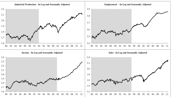
Argentina is a tough case, since none of the four coincident series were available on a monthly basis from January 1980 to June 2012. We used industrial production data from the Monthly Survey of Manufacture, released by Argentina’s National Institute of Statistics and Censuses (INDEC), available since 1994. This index is available for the entire industrial sector.

Employment data is particularly scarce in Argentina, since the broader series which covers the whole economy is available only quarterly since 2003. Longer series are available only in terms of the percentage of employed persons, and most of the sample only on a semiannual basis. Thus, the solution to approximate the number of employed people was to use the monthly number of employees in the supermarket sector, released by the INDEC since January 1997.

As a measure of income, we used an index of private nominal wages, which is extracted from the INDEC and constructed as a weighted average of indicators of the formal and the informal sectors. For the real income measure, the nominal index was deflated by the consumer prices index. Although the series is short as it is available since October 2001, it is the only indicator that displays a broad income measure of the economy.

In the case of an absent aggregate indicator of retail sales for the entire economy, we used data from INDEC’s Encuesta de Centros de Compras (Shopping Centers Survey), which covers thirty shopping centers since January 1997, about 50% of which are located in Buenos Aires.

To back-cast the coincident series, we used an auxiliary variable to interpolate GDP (Issler and Notini, 2008) to monthly frequency: the volume of monthly sales of cement provided by Association of Portland Cement since 1980. Those two series, interpolated GDP and cement sales, were then used as covariates in back-casting the series in the coincident index.

All four Argentina coincident series are plotted in Figure 1, which includes the results of the back-cast series. The non-shaded areas in the graphs depict the actual sample in which we observe them.

2_{The Quadratic Probability Score, labeled as QPS, is given by:}

QP S=

PT

t₌₁(Pt−Rt)2

T

(9)

Figure 1: Argentina’s Coincident Series

1,6 1,7 1,8 1,9 2,0 2,1 2,2

80 82 84 86 88 90 92 94 96 98 00 02 04 06 08 10 12 Industrial Production - In Log and Seasonally Adjusted

3,4 3,5 3,6 3,7 3,8 3,9

80 82 84 86 88 90 92 94 96 98 00 02 04 06 08 10 12 Employment - In Log and Seasonally Adjusted

1,2 1,4 1,6 1,8 2,0 2,2 2,4

80 82 84 86 88 90 92 94 96 98 00 02 04 06 08 10 12 Sales - In Log and Seasonally Adjusted

1,6 1,7 1,8 1,9 2,0 2,1 2,2 2,3 2,4

(10)

4.3. Brazil

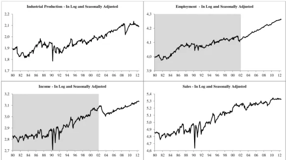
Here we follow Issler et al. (2012) in constructing our coincident series. The only difference regarding their work is that we update the data of their paper until June 2012 since their index had been only computed until November 2007. For output, we use industrial production computed by IBGE available from January 1980. As there is not a long span of sales series in Brazil, we thus use total Brazilian production of corrugated paper, which is computed by ABPO, as a proxy for sales. The employment measure is the total number of persons – 10 years old and above – who have a job according to IBGE’s Monthly Employment Survey, available since March 2002. The real income series, extracted from the same Survey, work as a proxy for income. The coincident series are plotted in Figure 2, which includes the results of the back-cast series. The non-shaded areas in the graphs depict the actual sample in which we observe them.

Figure 2: Brazil’s Coincident Series

3,9 4,0 4,1 4,2 4,3

4,6 4,7 4,8 4,9 5,0 5,1 5,2 5,3 5,4

2,7 2,8 2,9 3,0 3,1 3,2

80 82 84 86 88 90 92 94 96 98 00 02 04 06 08 10 12 Income - In Log and Seasonally Adjusted

1,7 1,8 1,9 2,0 2,1 2,2

(11)

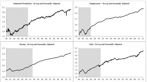
4.4. Chile

For employment, the general indicator of employment in the economy is used, available from Jan-uary 1986. For back-casting this series, the manufacturing employment series is used - available from the International Financial Statistics (IFS) database of the International Monetary Fund. In the case of income, we employ an index of real compensation per hour series published by the National Institute of Statistics (INE), which is available from April 1993. To back-cast it, we use as auxiliary variables the monthly GDP (Issler and Notini, 2008), employment in the manufacturing sector, and the industrial production index, both available since 1980 in the IMF database.

Retail sales, released by the “Camara Nacional del Comercio” (National Commerce Chamber) of Chile, is used as the sales proxy. It is available on a monthly basis since January 1991. To back-cast it, we chose as covariates monthly GDP and the employment in the manufacturing sector.

The industrial production index published by INE is available only since 1991. However, the IMF provides a monthly production series available since 1980 that was used as co-variate in the back-casting procedure.

The coincident series are plotted in Figure 3, which includes the results of the back-casted series. The non-shaded areas in the graphs depict the actual sample in which we observe them.

Figure 3: Chile’s Coincident Series

1,5 1,6 1,7 1,8 1,9 2,0 2,1

3,4 3,5 3,6 3,7 3,8 3,9

1,4 1,5 1,6 1,7 1,8 1,9 2,0 2,1 2,2

1,8 1,9 2,0 2,1 2,2 2,3

(12)

4.5. Colombia

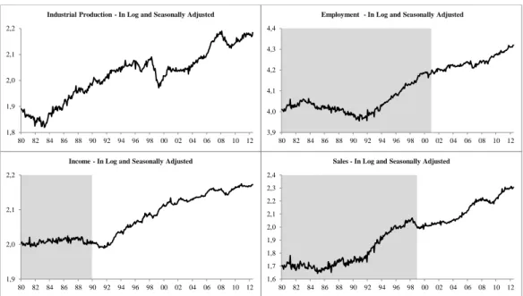
In the case of Colombia, the industrial production and income series were extracted from the Monthly Manufacturing Survey. The first series has been available since 1980, whereas the real in-come variable is available from 1990. The measure of retail sales is based on the Muestra Mensual de Comercio al por Menor (Monthly Retail Survey), which represents the actual sales excluding the share of fuel sales. The employment series is based on the total employment in the economy, which is monthly released in the Household Survey since 2001. All four series are published monthly by the National Administrative Department of Statistics (DANE).

To back-cast the employment and sales series, we used as covariates the industrial production index and the real imports of consumer and capital goods released monthly by DANE. The coincident series are plotted in Figure 4, which includes the results of the back-cast series. The non-shaded areas in the graphs depict the actual sample in which we observe them.

Figure 4: Colombia’s Coincident Series

1,8 1,9 2,0 2,1 2,2

3,9 4,0 4,1 4,2 4,3 4,4

1,6 1,7 1,8 1,9 2,0 2,1 2,2 2,3 2,4

1,9 2,0 2,1 2,2

(13)

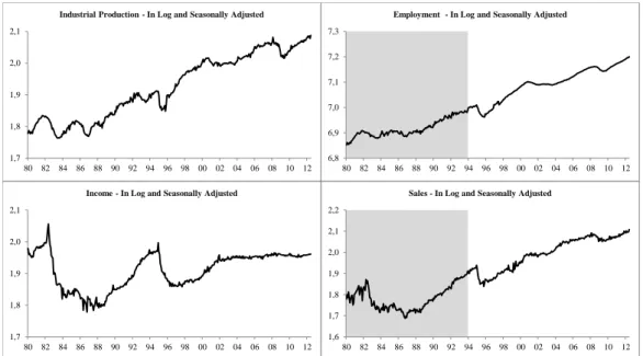
4.6. Mexico

The National Institute of Statistics and Geography (INEGI) releases a monthly coincident indicator, similar to the TCB index. In this work, we estimate the INEGI index from 1980.

The industrial production and nominal income series are available since 1980 in the INEGI’s Monthly Industrial Survey. In the second series, the monthly Consumer Price Index released by INEGI was em-ployed to deflate the nominal income and build the real income series. As in the Mexican case, there is not a broad survey of employment that covers the whole economy monthly. Therefore, the Insured Workers index, released since 1994 by the Secretary of Labor and Social Commercial Establishments was used. These last two series were back-casted.

To back-cast the series, we used the industrial production series, the income series and the interpo-lated monthly GDP (Issler and Notini). The coincident series are plotted in Figure 5, which includes the results of the back-casted series. The non-shaded areas in the graphs depict the actual sample in which we observe them.

Figure 5: Mexico’s Coincident Series

1,7 1,8 1,9 2,0 2,1

6,8 6,9 7,0 7,1 7,2 7,3

1,6 1,7 1,8 1,9 2,0 2,1 2,2

1,7 1,8 1,9 2,0 2,1

(14)

5. THE COINCIDENT INDICATOR

For each country, using the now available coincident series from 1980 through 2012, we constructed a coincident index using equation (1). Then, the turning points of each-country composite index was detected using the Bry and Boschan (1971) dating algorithm.

5.1. Argentina

In the case of Argentina, we have 7 recessions in the period, averaging one recession every 4.6 years. The average duration of the recessions is 12.7 months, one of the highest among the countries analyzed. Figure 7 shows the coincident indicator, with shaded areas depicting recession periods.

Figure 6: Argentina Coincident Index

80,0 90,0 100,0 110,0 120,0 130,0 140,0 150,0 160,0

80 82 84 86 88 90 92 94 96 98 00 02 04 06 08 10 12

Table 1 lists Argentina’s recessions from 1980:1 to 2012:06 when turning points dating is made using Bry and Boschan’s technique.

Table 1: Turning Points – Argentina

Peak Dates Through Dates Duration (months) Amplitude

1980:04 1981:05 14 3.14

1984:06 1985:08 15 3.59

1988:03 1990:03 25 9.49

1992:06 1992:11 6 1.12

1994:09 1995:09 13 4.49

2001:06 2002:03 10 6.24

(15)

5.2. Brazil

Brazil has the highest number of recessions of all Latin-American countries analyzed here: a total of ten. On the other hand, the average length of these recessions is low: 10.6 months. In other words, Brazil had shorter cycles (expansions and recessions), but are more frequent. Figure 7 presents the Brazilian coincident indicator. On average, Brazil had one recession every three years.

Figure 7: Brazil Coincident Index

90,0 95,0 100,0 105,0 110,0 115,0 120,0 125,0 130,0

80 82 84 86 88 90 92 94 96 98 00 02 04 06 08 10 12

The turning points of Brazilian business cycles are summarized in Table 2.

Table 2: Turning Points – Brazil

1980:10 1981:09 12 3.63

1982:07 1983:02 8 2.2

1987:02 1988:10 21 4.38

1989:08 1990:04 9 11.43

1991:07 1991:12 6 4.92

1994:12 1995:07 8 4.56

1997:10 1999:02 17 1.98

2000:12 2001:09 10 2.66

2002:10 2003:06 9 2.48

(16)

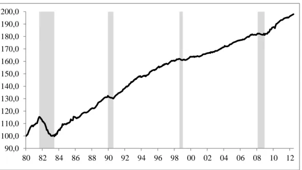
5.3. Chile

The Chilean economy has the smoother trend growth among all countries analyzed here. During the more than 32 years we focus on, there were four recessions lasting about 12 months each. However, there was only one severe recession, as Figure 8 shows.

Figure 8: Chile Coincident Index

90,0 100,0 110,0 120,0 130,0 140,0 150,0 160,0 170,0 180,0 190,0 200,0

80 82 84 86 88 90 92 94 96 98 00 02 04 06 08 10 12

The turning points are summarized in Table 3.

Table 3: Turning Points – Chile

1981:08 1983:06 23 15.62

1989:12 1990:08 9 2.21

1998:08 1999:01 6 0.98

(17)

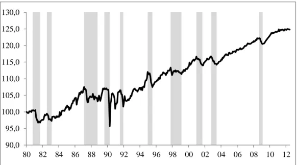
5.4. Colombia

The Colombian economy showed eight recessions from 1980 to 2012, with an average of one re-cession every four years. Among the analyzed countries, Colombia was the economy with the lowest average recession duration: 10 months. Figure 9 shows the coincident indicator, where the shaded areas correspond to the recession’s periods.

Figure 9: Colombia Coincident Index

90,0 100,0 110,0 120,0 130,0 140,0

80 82 84 86 88 90 92 94 96 98 00 02 04 06 08 10 12

The Colombia turning points are summarized in Table 4.

Table 4: Turning Points – Colombia

1981:03 1981:12 10 4.85

1983:10 1985:01 16 2.43

1988:07 1988:12 6 3.27

1990:03 1991:04 14 2.25

1998:04 1998:12 9 2.87

2000:12 2001:05 6 1.13

(18)

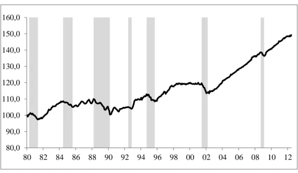
5.5. Mexico

The Mexican economy shows the highest average recession’s duration among the countries ana-lyzed. From 1980 to 2012, six recessions were recorded, which lasted 14.5 months, on average. Figure 10 shows the coincident indicator, where recessions periods are depicted by shaded areas.

Figure 10: Mexico Coincident Index

90,0 100,0 110,0 120,0 130,0 140,0 150,0

80 82 84 86 88 90 92 94 96 98 00 02 04 06 08 10 12

Mexico’s turning points are summarized in Table 5.

Table 5: Turning Points – Mexico

1982:04 1983:11 20 12.18

1985:07 1986:10 16 6.39

1987:11 1988:07 9 2.29

1994:12 1995:10 11 10.85

2000:08 2001:10 15 1.12

(19)

5.6. Latin America

After building and analyzing each country indicators, we propose a Latin America aggregate indi-cator, where each country was weighted by their respective standard deviation, using the idea behind equation (1). Figure 11 shows the Latin America indicator, where shaded areas depict recession periods.

Figure 11: Latin America Coincident Index

90,0 100,0 110,0 120,0 130,0 140,0 150,0 160,0 170,0 180,0

80 82 84 86 88 90 92 94 96 98 00 02 04 06 08 10 12

Latin America: Coincident Index

There were common recession periods in the early 1980’s, where several countries faced balance of payments problems as a result of fixed exchange rate regimes combined to the global financial insta-bility brought by the two oil shocks. Another region common recession period was the one followed by the Mexican crisis, which hit many emerging economies due to the confidence crisis and increased investor risk aversion. Finally, the 2000-02 recessions impact most countries due to the global nature of the crisis, which started with the bursting of the technology sector bubble.

Regarding the 2008 global financial crisis, the Mexican economy was the most affected because of its heavy dependence on the U.S. economic cycle. However, all the economies in the region suffered with the global slowdown after a while. Despite that, at the beginning of the 2008 crisis, which first hit first the more mature economies, some authors believed that emerging economies would decouple from advanced economies. This proved to be wrong, but only after a while. It is relevant to test empirically whether there is any relationship between the Latin America coincident indicator and the United States indicator. Both are presented in Figure 12.

We now examine whether there is Granger-causality between the coincident index of the U.S. (TCB) and our Proposed Latin-American coincident index. The two do not cointegrate. Thus, we take the first-difference of the two series prior to performing Granger-causality tests using the Sims version of the test. The lag length chose were 3 and 6, both are optimally chosen by different information criteria. The

results are clear: the U.S. coincident indicatorGranger-causesthe Latin-American coincident indicator,

but it is notGranger-causedby it. This means that the U.S. index is a good leading indicator for Latin

(20)

Figure 12: US and Latin America Coincident Indexes

90 100 110 120 130 140 150 160 170 180 190 200

80 82 84 86 88 90 92 94 96 98 00 02 04 06 08 10 12 Latin America United States

5.6.1. Business Cycle Synchronization

Finally, we investigate the degree of business-cycle synchronization across the Latin-American coun-tries applying the Concordance Index (CI) proposed by Harding and Pagan (2002). The CI measures the

degree of co-movement between one country/region specific cycle (yjt) and other country/region

cy-cle (yrt). It counts the fraction of time both series are simultaneously in the same state of expansion

(St= 1) or contraction (St= 0). Mathematically, for a total ofnperiods, we compute the concordance

index to be:

Ijr=n−1

h

#Sjt= 1, Srt = 1 i+n−1

h

#Sjt= 0,Srt= 0 i (10)

(21)

Table 6: Harding and Pagan (2002) Concordance Index

Argentina Brazil Chile Colombia Mexico Latin America

Argentina 1 0.72 0.69 0.70 0.69 0.78

Brazil 1 0.73 0.71 0.72 0.77

Chile 1 0.83 0.78 0.91

Colombia 1 0.78 0.74

Mexico 1 0.82

Latin America 1

6. CONCLUSION

This paper has three main contributions. The first is to propose a coincident indicator for specific Latin American countries: Argentina, Brazil, Chile, Colombia and Mexico.

In order to obtain similar series to those defined by The Conference Board (TCB) when constructing coincident indices (output, sales, income and employment), we chose to back-cast various individual country series. When back-casting, we followed Issler et al. (2012), who proposed a state-space proce-dure based on the interpolation method of Bernanke et al. (1997) and the extensions made by Mönch and Uhlig (2005).

The second contribution is to establish a chronology of recessions for these countries, covering the period from 1980 to 2012 on a monthly basis. These results are validated comparing the quarterly chronology of recessions using official GDP data and the coincident series constructed. The last contri-bution is to propose an aggregate indicator for the Latin American economy, weighting the individual composite indicators for the five countries analyzed here.

The composite regional index for Latin America tracks reasonably well its economic activity, al-though not all countries follow the behavior of the composite index. For the countries surveyed, on average, recessions are more frequent than in the U.S., the only exception being Chile. Regarding the magnitude of the 2007/2008 global financial crisis, all five countries were affected. Finally, a chronology of recessions in Latin America was established and the Latin-American cycles were compared to the U.S.

business cycles, finding that the U.S. cycleGranger-causesthe Latin American cycle but it is not caused

(22)

BIBLIOGRAPHY

Aiolfi, M., Catão, L., & Timmerman, A. (2011). Common factor in Latin America’s business cycles.Journal

of Development Economics, 95(2):212–228.

Artis, M. J., Kontolemis, Z. G., & Osborn, D. R. (1997). Business cycles for G7 and European countries.

Journal of Business, 70(2):249–279.

Backus, D. & Kehoe, P. (1992). International evidence on the historical properties of business cycles.

American Economic Review, 82:864–888.

Bernanke, B., Gertler, M., & Watson, M. (1997). Systematic monetary policy and the effects of oil price

shocks.Brookings Papers on Economic Activity, pages 91–157.

Boldin, M. D. (1994). Dating turning points in the business cycles.Journal of Business, 67(1):97–130.

Bry, G. & Boschan, C. (1971). Cyclical Analysis of Time Series: Selected Procedures and Computer Programs.

Columbia University Press, New York.

Burns, A. F. & Mitchell, W. C. (1946). Measuring Business Cycles. National Bureau of Economic Research,

New York.

Calvo, G. A., Leiderman, L., & Reinhart, C. (1992). Capital inflows and real exchange rate appreciation in

Latin America: The role of external factors. IMF Staff Papers, 40(1):108–151.

Chauvet, M. (1998). An econometric characterization of business cycle dynamics with factor structure

and regime switching.International Economic Review, 39:969–996.

Chauvet, M. (2001). A monthly indicator of Brazilian GDP.Brazilian Review of Econometrics, 21:1–48.

Chauvet, M. (2002). The Brazilian business cycle and growth cycles. Revista Brasileira de Economia,

56:75–106.

Chauvet, M., Lima, E., & Vasquez, B. (2002). Forecasting Brazilian output in real time in the presence of breaks: A comparison of linear and non-linear models. Texto para Discussão 11, IPEA.

Chauvet, M. & Piger., J. M. (2008). A comparison of the real-time performance of business cycle dating

methods.Journal of Business and Economic Statistics, 26:42–49.

Contador, C. & Ferraz, C. (1999). Previsão com Indicadores Antecedentes. Silcon, Rio de Janeiro.

Contador, C. & Haddad, C. (1975). Produto real, moeda e preços: A experiência brasileira no período

1861-1970. Revista Brasileira de Estatística, Jul/Set:407–440.

Contador, R. C. (1977).Ciclos Econômicos e Indicadores de Atividade. INPES/IPEA, Rio de Janeiro.

Correa, A. S. (2003). Diferenças entre países da América Latina: Uma análise de Markov-Switching para os ciclos econômicos de Brasil e Argentina. Trabalho para Discussão 80, Banco Central do Brasil.

Duarte, A. J. M., Issler, J. V., & Spacov, A. (2004). Coincident indices of economic activity and a chronology

of Brazilian recessions. Pesquisa e Planejamento Econômico, 34(1):1–37.

Engle, R. & Issler, J. (1993). Common trends and common cycles in Latin America. Revista Brasileira de

Economia, 47(2):149–176.

Engle, R. F. & Granger, C. (1987). Cointegration and error correction: Representation, estimation and

(23)

Estrella, A. & Mishkin, F. (1999). Predicting U.S. recessions: Financial variables as leading indicators.

Review of Economics and Statistics, 80:45–61.

Forni, M., Hallin, M., Lippi, M., & Reichlin, L. (2000). The generalized dynamic factor model:

Identifica-tion and estimaIdentifica-tion. The Review of Economics and Statistics, 82(4):540–554.

Hamilton, J. D. (1989). A new approach to the economic analysis of nonstationary time-series and the

business cycle. Econometrica, 57(2):357–384.

Harding, D. & Pagan, A. (2002). Dissecting the cycle: A methodological investigation.Journal of Monetary

Economics, 49(2):365–381.

Harvey, A. (1989). Forecasting, Structural Time Series and the Kalman Filter. Cambridge University Press,

Cambridge.

Harvey, A. C. & Pierse, R. G. (1984). Estimating missing observations in economic time series.Journal of

the American Statistical Association, 79:125–131.

Hecq, A., Palm, F. C., & Urbain, J.-P. (2006). Common cyclical features analysis in VAR models with

cointegration. Journal of Econometrics, 132(1):117–141.

Hollauer, G., Issler, J., & Notini, H. (2009). Novo indicador coincidente para a atividade industrial

brasileira.Revista de Economia Aplicada, 13:5–28.

Issler, J. V. & Notini, H. (2008). Estimating Brazilian monthly real GDP: A Kalman filter approach. Mimeo, FGV/EPGE.

Issler, J. V., Notini, H., & Rodrigues, C. (2012). Constructing coincident and leading indices of economic

activity for the Brazilian economy. Journal of Business Cycles Measurement and Analysis, 2012:2.

Issler, J. V. & Spacov, A. D. (2000). Usando correlações canônicas para identificar indicadores antecedentes e coincidentes da atividade econômica no Brasil. Relatório de pesquisa, Mimeo.

Issler, J. V. & Vahid, F. (2006). The missing link: Using the NBER recession indicator to construct

coinci-dent and leading indices of economic activity.Journal of Econometrics, 132(1):281–303.

Kwiatkowski, D., Phillips, P. C. B., Schmidt, P., & Shin, Y. (1992). Testing the null hypothesis of stationarity against the alternative of a unit root: How sure are we that economic time series have a unit root?

Journal of Econometrics, 54:159–178.

Kydland, F. & Zarazaga, C. E. (1997). Is the business cycle of Argentina different? Federal Reserve Bank

of Dallas, Fourth Quarter, pp. 21–36,Economic Review.

Lucas, R. E. (1977). Understanding business cycles. Carnegie-Rochester Conference Series on Public Policy,

5:7–29.

Marcelino, M. (2006). Leading indicators: What have we learned? Technical Report 4977, CEPR Discus-sion Papers.

Mariano, R. & Murasawa, Y. (2003). A new coincident index of business cycles based on monthly and

quarterly series. Journal of Applied Econometrics, 18:427–443.

Mönch, E. & Uhlig, H. (2005). Towards a monthly business cycle chronology for the Euro area.Journal of

Business Cycle Measurement and Analysis, 1(2):43–69.

(24)

Neumeyer, P. & Perri, F. (2005). Business cycles in emerging economies: The role of interest rates.Journal of Monetary Economics, 52(2):345–380.

Newey, W. & West, K. (1987). A simple positive semi-definite, heteroskedascity and autocorrelation

consistent covariance matrix. Econometrica, 55:703–708.

Phillips, P. & Perron, P. (1988). Testing for a unit root in time series regression. Biometrika, 75:335–346.

Picchetti, P. & Toledo, C. (2002). Estimating and interpreting a common stochastic component for the

Brazilian industrial production index. Revista Brasileira de Economia, 56:107–120.

Spacov, A. (2000). Índices antecedentes e coincidentes de atividade econômica brasileira: Uma aplicação da análise de correlação canônica. FGV/EPGE, Dissertação de Mestrado.

Stock, J. & Watson, M. (1988a). A new approach to leading economic indicators. Mimeo, Harvard University, Kennedy School of Government.

Stock, J. & Watson, M. (1988b). A probability model of the coincident economic indicator. Technical Report 2772, NBER Working Paper.

Stock, J. & Watson, M. (1989). New indexes of coincident and leading economic indicators. InNBER

Macroeconomics Annual, pages 351–395. MIT Press.

Stock, J. & Watson, M. (1993a). New research on business cycles, indicators and forecasting. InNew

Research on Business Cycles, Indicators and Forecasting. University of Chicago Press, for NBER.

Stock, J. & Watson, M. (1993b). A procedure for predicting recessions with leading indicators:

Econo-metric issues and recent experience. In Stock, J. H. & Watson, M. W., editors,New research on business

cycles, indicators and forecasting. University of Chicago Press, for NBER, Chicago.

Stock, J. & Watson, M. W. (1991). A probability model of the coincident economic indicator. In Lahiri, K. &

Moore, G. H., editors,Leading Economic Indicators: New Approaches and Forecasting Records. Cambridge

University Press, Cambridge.

Uribe, M. & Yue, V. (2006). Country spreads and emerging countries: Who drive whom? Journal of

International Economics, 60:6–36.

Vahid, F. & Engle, R. F. (1993). Common trends and common cycles. Journal of Applied Econometrics,

8:341–360.

Vahid, F. & Issler, J. V. (2002). The importance of common-cyclical features in VAR analysis: A Monte

Carlo study.Journal of Econometrics, 109:341–363.

Zarnowitz, V. (1981). Business cycles and growth: Some reflections and measures. Technical Report 665, Working Papers.

Zarnowitz, V. (1985). Recent work on business cycles in historical perspective: Review of theories and evidence. Technical Report 1503, NBER Working Papers.

(25)

A. APPEDINX TABLES

Table A-1: Coincident Series - Description

Country Series Name Description Sample Period Source

Argentina

Employment Employment in the supermarket sector 1997:01 - 2012:06 MECON Income Nominal Wages index deflated by CPI 2001:10 - 2012:06 INDEC Industrial Production Industrial Production Index 1994:01 - 2012:06 INDEC Sales Shopping Center Sales deflated by CPI 1997:01 - 2012:06 INDEC

Brazil

Employment Total Employment in metropolitan areas 2002:03 - 2012:06 IBGE

Income Real Average wage index 2002:03 - 2012:06 IBGE

Industrial Production Industrial Production Index 1980:01 - 2012:06 IBGE

Sales Production of Corrugated paper 1980:01 - 2012:06 IBGE

Chile

Employment Total national employment 1986:01 - 2012:06 INE

Income Real compensation per hour 1993:04 - 2012:06 INE

Industrial Production Industrial Production Index 1991:01 - 2012:06 INE

Sales Real Retail Sales 1991:01 - 2012:06 CNC

Colombia

Employment Total national employment 2001:01 - 2012:06 DANE

Income Real wages in manufacturing sector 1990:01 - 2012:06 DANE

Industrial Production Industrial Production Index 1980:01 - 2012:06 DANE

Sales Real Retail Sales excluding fuel 1999:01 - 2012:06 DANE

Mexico

Employment Insured Workers 1994:01 - 2012:06 Secretary of Labor

and Social Security Income Nominal Wages index deflated by CPI 1980:01 - 2012:06 INEGI Industrial Production Industrial Production Index 1980:01 - 2012:06 INEGI

Sales Real Retail Sales 1994:01 - 2012:06 INEGI

Table A-2: Covariates - Description

Country Covariates Sample Period Source

Argentina Cement Production 1980:01 - 2012:06 Association of Portland Cement Monthly GDP 1980:01 - 2012:06 Estimated using Issler and Notini (2008)

Brazil

Corrugated Paper Production 1980:01 - 2012:06 ABPO

Energy Production 1980:01 - 2012:06 NOS

Cement Production 1980:01 - 2012:06 SNIC

Monthly GDP 1980:01 - 2012:06 Estimated using Issler and Notini (2008)

Chile

Manufacturing Employment 1980:01 - 2006:03 IMF/IFS

Industrial Production 1980:01 - 2011:12 IMF/IFS

Monthly GDP 1980:01 - 2012:06 Estimated using Issler and Notini (2008)

Colombia

Industrial Production 1980:01 - 2012:06 DANE

Manufacturing Employment 1980:01 - 2012:06 DANE

Real Capital Goods Imports 1980:01 - 2012:06 DANE Real Consumer Goods Imports 1980:01 - 2012:06 DANE

Mexico

Industrial Production 1980:01 - 2012:06 INEGI

Income 1980:01 - 2012:06 INEGI

(26)

Table A-3: Backcasted Series - Description

Country Backcasted Series Covariates Backcasting Period

Argentina

Employment Monthly GDP and Cement Production 1980:01 - 1996:12 Income Monthly GDP and Cement Production 1980:01 - 2001:09 Industrial Production Monthly GDP and Cement Production 1980:01 - 1993:12 Sales Monthly GDP and Cement Production 1980:01 - 1996:12

Brazil Employment Monthly GDP and Energy Production 1980:01 - 2002:02 Income Corrugated Paper and Cement Production 1980:01 - 2002:02

Chile

Employment Manufacturing Employment 1980:01 - 1985:12

Income Industrial Production, Manufacturing 1980:01 - 1993:03 Employment and Monthly GDP

Industrial Production Industrial Production 1980:01 - 1990:12

Sales Industrial Production and Manufacturing 1980:01 - 1990:12 Employment

Colombia

Employment

Industrial Production, Manufacturing

1980:01 - 2000:12 Employment, Real Imports of Capital

and Consumer Goods

Income Manufacturing Employment and Real 1980:01 - 1989:12 Imports of Consumer Goods

Sales Industrial Production, Manufacturing 1980:01 - 1998:12 Employment, Real Imports of Capital

and Consumer Goods

Mexico Employment

Industrial Production, Real Income and

1980:01 - 1993:12 Monthly GDP

(27)

Table A-4: Coincident Series - Unit Root Tests

Country Series Name ADF Kwiatkowski et al Phillips and Perron

t-statistic p-value L M-statistic t-statistic p-value

Argentina

Employment 0,157 0,970 2.12∗ _0,134 _0,968

Income 0,052 0,962 2.09∗ _0,248 _0,975

Industrial Production 2,112 1,000 1.82∗ _2,121 _1,000

Sales 1,000 0,997 1.84∗ _1,492 _0,999

Brazil

Employment 0,238 0,975 2.21∗ _0,301 _0,978

Income -1,061 0,732 2.11∗ _-0,772 _0,825

Industrial Production -0,188 0,937 2.32∗ _-0,449 _0,898

Sales -1,140 0,701 2.34∗ _-0,521 _0,884

Chile

Employment -0,821 0,812 2.26∗ _-1,602 _0,481

Income -0,379 0,910 2.31∗ _-0,237 _0,931

Sales -0,628 0,861 2.31∗ _-0,747 _0,832

Colombia

Employment 0,984 0,997 2.15∗ _0,870 _0,995

Income -0,381 0,909 2.09∗ _-0,414 _0,904

Sales 0,686 0,992 2.30∗ _0,551 _0,988

Mexico

Employment 0,065 0,963 2.38∗ _-0,038 _0,954

Income -0,398 0,907 2.33∗ _-0,515 _0,885

Industrial Production -1,301 0,631 0.73∗ _-1,826 _0,368

Sales -0,100 0,947 2.24∗ _-0,110 _0,946

Notes:(i) ADF and Phillips and Perron : series has a unit root; Kwiatkowski : series is stationary. (ii) the asterisk (*) indicates that we reject the null hypothesis at 5%.

Table A-5: Quarterly Turning Points - Argentina

Quarterly GDP Quarterly Coincident Index

Peak Dates Through Dates Duration Peak Dates Through Dates Duration

(quraters) (quraters)

1980:3 1982:2 7 <NA> 1981:2 NA

1984:2 1985:3 5 1984:2 1985:3 5

1987:3 1990:1 10 1987:3 1990:2 11

1994:4 1995:3 3 1992:2 1992:4 2

1998:2 2000:3 9 1994:4 1995:4 4

2001:1 2002:1 4 1998:3 1999:3 4

2008:3 2009:2 3 2000:1 2002:1 8

(28)

Table A-6: Quarterly Turning Points - Brazil

1980:4 1981:4 4 1980:4 1981:3 3

1982:3 1983:1 2 1982:3 1983:1 2

1988:1 1988:4 3 1987:1 1987:3 2

1989:3 1990:2 3 1989:4 1990:2 2

1991:3 1992:3 4 1991:3 1992:2 3

1995:1 1995:3 2 1995:1 1995:3 2

1998:2 1998:4 2 1997:3 1999:1 6

2001:1 2001:4 3 2000:4 2001:3 3

2002:4 2003:2 2 2002:3 2003:2 3

2008:3 2009:1 2 2008:3 2009:1 2

Table A-7: Quarterly Turning Points - Chile

1981:3 1982:4 5 1981:3 1983:1 6

1990:1 1990:3 2 1989:4 1990:3 3

1998:2 1999:1 3 1998:3 1999:2 3

(29)

Table A-8: Quarterly Turning Points - Colombia

1998:2 1999:2 4 <NA> 1980:3 NA

1981:1 1982:1 4

1982:3 1983:2 3

1983:4 1985:1 5

1987:4 1988:4 4

1990:1 1991:2 5

1995:4 1996:4 4

1998:1 1999:1 4

2000:4 2001:2 2

2002:2 2002:4 2

2008:1 2008:4 3

Note: Quarterly GDP data for Colombia is available only since 1994

Table A-9: Quarterly Turning Points - Mexico

1981:4 1983:2 6 1982:2 1983:4 6

1985:3 1986:4 5 1985:1 1986:4 7

1987:4 1988:3 3 1987:4 1988:3 3

1994:4 1995:2 2 1994:4 1995:3 3

2002:2 2003:1 3 2000:3 2002:1 6

2008:2 2009:2 4 2008:1 2009:2 5

Table A-10: Average Economy-state forecast Error (QPS)

Country Peaks Throughs

Argentina 4.62% 8.46%

Brazil 7.69% 7.69%

Chile 4.62% 4.62%

Colombia 8.11% 8.11%

(30)

Table A-11: Bernanke, Gertler, and Watson measures of fit

Country Backasted series R

2

Level Diff

Argentina

Employment 0.2012 0.2128

Income 0.1448 0.1453

Industrial Production 0.4381 0.4402

Sales 0.2050 0.2060

Brazil Employment 0.5968 0.5979

Income 0.6634 0.6651

Chile

Income 0.7070 0.7088

Industrial Production 0.7567 0.7589

Sales 0.4441 0.4475

Colombia

Income 0.4959 0.5020

Sales 0.6187 0.6204

Mexico Employment 0.5071 0.5092