Recebido em 13/dezembro/2011 Aprovado em 11/novembro/2014
Sistema de Avaliação: Double Blind Review
Editor Cientíico: Nicolau Reinhard
DOI: 10.5700/rausp1181
R
ESU
MO
Rodrigo Menon Simões Moita, Mestre em Economia pela Universidade de São Paulo, Doutor em Economia pela Universidade de Illinois em Urbana- -Champaign (Estados Unidos), é Professor do Insper (CEP 04546-042 – São Paulo/SP, Brasil). E-mail: [email protected]
Endereço: Insper
Rua Quatá, 300 – Sala 418 04546-042 – São Paulo – SP
Carlos Eduardo Lobo e Silva, Economista pela Universidade de São Paulo, Mestre em Economia Aplicada pela Universidade de São Paulo e Ph.D. em Planejamento Regional pela Universidade de Illinois em Urbana-Champaign, é Professor da Pontifícia Universidade Católica do Rio Grande do Sul (CEP 90619-900 – Porto Alegre/RS, Brasil). E-mail: [email protected]
Eduardo de Carvalho Andrade, Bacharel e Mestre em Economia pela Pontifícia Universidade Católica do Rio de Janeiro, Ph.D. em Economia pela Universidade de Chicago, é Economista e Sócio da Apex Capital Ltda. (CEP 04547-004 – São Paulo/SP, Brasil).
E-mail: [email protected]
Permanent demand excess as business
strategy: an analysis of the Brazilian
higher-education market
Rodrigo Menon Simões Moita Insper – São Paulo/SP, Brasil
Carlos Eduardo Lobo e Silva
Pontifícia Universidade Católica do Rio Grande do Sul – Porto Alegre/RS, Brasil
Eduardo de Carvalho Andrade Apex Capital Ltda. – São Paulo/SP, Brasil
Excesso de demanda permanente como estratégia de mercado: uma análise do mercado brasileiro de ensino superior
Muitas Instituições de Ensino Superior (IES) preciicam seus
cursos abaixo do preço de equilíbrio para gerar excesso de
demanda permanente. Neste artigo, primeiramente se adaptam
as ideias de Becker (1991) para entender por que as IES
pre-ciicam seus cursos dessa maneira. O fato de os alunos serem consumidores e insumos no processo de produção de educação gera um equilíbrio de mercado em que algumas irmas cobram preços elevados e têm excesso de demanda por suas vagas, e outras cobram um preço baixo e sobram vagas. Em seguida, analisa-se esse equilíbrio empiricamente. Estima-se a demanda por cursos de graduação em Administração no estado de São Paulo. Os resultados mostram que o preço, a qualidade dos alu
-nos ingressantes e a porcentagem de professores com doutorado são os fatores determinantes na escolha de um estudante. Dado que a qualidade dos estudantes determina a demanda por uma IES, calcula-se qual é o valor, para uma IES, de ter melhores estudantes. Esse valor é igual à receita de que ela abdica para manter excesso de demanda e seleção de alunos. Com respeito
ao investimento em seleção de alunos, 39 IES no estado de
São Paulo abdicaram de uma receita de aproximadamente R$ 5 milhões por ano por turma de ingressantes, o que equivale a 7,6% da receita de uma classe de ingressantes.
1. INTRODUCTION
Microeconomics manuals teach that, in equilibrium, the amount demanded for a good or service must equal the amount supplied. In the higher-education market, this principle does not hold. Instead, many higher-education institutions (HEIs) limit the number of available slots to guarantee permanent excess demand. The same phenomenon can be observed in other markets, especially service markets, but the rationale behind excess demand in higher education does not apply to restaurants or large events. In education, the student is not only the consumer, but also he or she is a factor of production. As consequence, the quality of the output is a function of the quality of the student body. For this reason, given the characteristics of HEI and the quantity of available slots, the institution charges tuition below equilibrium price to increase the quantity of appliers and, thus, to beneit from greater selectivity.
The Brazilian market for HEIs is predominantly composed by private enterprises. Among 2.281 HEIs in 2006, 89% were private, and 74.6% of all students were enrolled in these private schools. Additionally, the majority of private HEIs (52%) are for proit (2006 Higher Education Census – Ministry of Education). Despite the lack of oficial data on the amount of donations received by HEIs, it is known that the resources derived from this source are limited, as are the resources available to fund research. In this context, most Brazilian private HEIs primarily raise funds from student tuition payments. Those are little known outside their area and, although they charge low tuitions, have empty slots. They coexist with some HEIs with good reputation, which charge high tuitions and have hotly disputed selection processes. Among private Business Administration schools in São Paulo in 2006, for example, the fees range from R$ 170 to R$ 2.250 (or from US$ 106 to US$ 1,415(1)), and the ratio of candidates to slots ranges from 0.17 to 11.5.
The sector has been going through substantial transformation over the last years. There has been a large increase in the number of students enrolled in higher education: from 1.3 million in 1995 to 3.8 million students in 2003 and 7.0 million in 2012 (2012 Higher Education Census – Ministry of Education). Despite the consistent growth observed over the last decades, there has been a substantial slowdown in the growth rate. The number of enrolled students more than tripled from 1995 to 2003, while it less than doubled from 2003 to 2012.
The players and their size have also changed. A fast consolidation process has taken place, with some large educational groups (Anhanguera, Estacio and Kroton, among others) buying local institutions. So, the observed trend nowadays is from a market with local and independent HEIs to a market dominated by large chains. Kroton and Anhanguera had 11% of the Brazilian market in 2011, and 14% in 2012, which means a growth of 27% in one year. However, the majority of supply still comes from local and independent institutions.
This article analyzes the HEI market and attempts to answer four interrelated questions:
• How do we theoretically understand the existence of the HEI that opts for the strategy of maintaining permanent excess demand?
• Which HEIs’ characteristics affect the demand for their business courses?
• How big is the group of HEIs that really invest in selectivity? • How much revenue does the HEI give up to increase the
selectivity of its admissions process and, consequently, the quality of its students?
Through two adaptations of the ideas of Becker (1991), we attempt to explain why some HEIs maintain permanent excess demand while others do not. Next, using a database of business schools in the state of São Paulo(2) (see section 3 for a detailed description of the dataset) we estimate the demand for higher education. The empirical results show that the quality of the student body, the tuition, and the quality of the lecturers are relevant in determining the demand of the market. The relevance of the quality of the student body justiies the strategy of an HEI that opts for excess demand and conirms the theory that will be developed in the next section: demand for the school hinges on the quality of the students and, ultimately, responds positively to the selectivity imposed by the HEI. Finally, using the results of econometric models, we present the total “investment” in selectivity made by São Paulo HEIs in their business programs. This total, which surpasses R$ 5 million (or US$ 3.14 million – 7.6% of the revenue) per year, can be understood as an investment in differentiation.
While Becker (1991) theoretically shows why some restaurants having long queues for tables do not raise prices, this paper estimates the “investment on queues”. The higher education market is specially appropriated for this study because there is data about all the candidates, including those students that failed in the selecting process. In a restaurant--market context, it would be as if we knew the numbers of
clients and the number of people who give up eating at a given
restaurant because of its long queues.
The selection of better students in higher education is well documented by literature, but how to measure its impact on the
education output is a controversial question (see Winston &
Zimmerman, 2003). Instead of measuring this effect, the focus of this work is to better understand how the existence of those
effects modiies the market equilibrium. Thus, we estimate (a) on one side, how the selectivity of HEIs (considering the quality of incoming students as a proxy) affects the demand curve, and (b) on the other side, how much the HEIs invest in selectivity to maximize their long term proits by maintaining permanent excess demand.
Bishop (1977) analyzes the decisions of high school students. He found that tuition has a more severe negative impact on lower income groups. Ehrenberg (2004) presents a review of this literature, corroborating the notion that a higher tuition and fewer inancial incentives, such as scholarships, reduce the motivation to study at an HEI. Other characteristics that may affect student preferences are less studied.
Another branch of this literature (Belzil & Hansen, 2002; Hartog & Diaz-Serrano, 2007; among others) analyzes higher education as an investment, and how earnings risk affects students’ choice. The results are not conclusive: Belzi and Hansen find a positive correlation between risk and the decision to attend college, while other authors ind a negative relationship.
Four papers follow this line of research and are closely related to our study. Gallego and Hernando (2008) also use a discrete choice model in Chilean high schools to estimate the effects of the voucher system on student well-being and socio--economic segregation. Monks and Ehrenberg (1999) use panel data to evaluate the impact on the demand for universities of the U.S. News and World Report rankings, the most traditional ranking in the U.S market. They conclude that a lower position in the ranking is detrimental to the university: fewer accepted students decide to enroll; the quality of new classes decreases, as measured by the admissions test; and the net tuition paid by the student is lower because the university has to be more generous in granting inancial aid to attract students from the smaller group of applicants.
Long (2004) examines how different cohorts of students in the United States choose which HEI to attend based on their own characteristics and those of the HEI, such as tuition, quality of the student body, percentage of lecturers with doctorates and student/lecturer ratio. Long’s study concludes that the quality of the faculty is the most important factor in the student’s decision, a result we also ind here.
Kelchtermans and Verboven (2009) study college choice in the Belgium region of Flandres. They conclude that courses are close substitutes, and that a tuition increase would not affect the decision of whether to study but affect the decision of where to study.
Flannery and O’Donoghue (2013) use a nested logit model with three choices: to attend college, to work or to work and study part time. They recognize two key features. First, college choice is a discrete choice problem where tuition and college quality variables are important in students’ choices. Second, there is a trade off between studying and working.
Other papers – such as Frenette (2009), Chowdry, Crawford, Dearden, Goodman, and Vignoles (2010), Spiess and Wrohlich (2010), among many others – investigate different aspects that affect college attendance. Despite the fact that all these papers also estimate a demand for educational institutions, the details of the method we employ and our goals are quite distinct from the others. We chose to restrict our analysis to
business administration courses only. Implicitly, we assume that business administration is not a substitute with other courses, such as biology or engineering. Moreover, our inal goal is both to identify the group of HEIs that invest in selectivity and to estimate the investment.
The rest of this article is organized as follows. In the next section, we discuss why a HEI could use the strategy to operate with excess demand. Sections 3 and 4 explains the methodology and data employed. The results are presented in Section 5. The inal section concludes the analysis.
2. THEORETICAL DISCUSSION
The fundamental hypothesis of Becker (1991), who studies the causes of excess demand in the restaurant industry, is that the individual’s demand depends on the other individuals’ demand. The author suggests that eating out, attending a cultural event or discussing a book are social activities in which people consume the product or service together, and therefore, the number of people sharing the same product inluences the utility of the individual consumer.
While in Becker’s model the decision of attending a cultural event is a function of the queues’ size because of social aspects; in the present paper, the choice of a HEI depends on the HEI’s capacity of selecting the best students. In both situations, excess demand creates demand.
More speciically, in the case of higher education, we claim that the Becker’s argument becomes even stronger because both the actual quality and the reputation of a graduate course are functions of the quality of its students. In terms of quality for enrolled students, the qualiication and performance of the cohort affect learning (the peer effect, which does not occur in the case of restaurants). Also the success of the graduates serves as signals to the market of the quality of the HEI. Therefore, excess demand allows HEI to select good students, who tend to be good graduates, which contribute to the reputation of the institution. Thus, in contrast with restaurants, the quality of enrolled students is fundamental to the choice of the potential students. Because greater selectivity increases the quality of the incoming class, we may conclude that excess demand creates demand, which should be considered in the maximization process of long-term proit. As result, the long-term equilibrium may present permanent excess demand.
In any market, one should expect higher demand for high--quality products than for lowhigh--quality products given the same price. However, in a “traditional” market, the equilibrium is reached by increasing price of high-quality products until eliminating excess demand.
This differentiation seems important with respect to higher education because we assume that permanent excess demand builds the HEI’s reputation, which in turn determines its short--term demand curve. The idea is that, in the short term, tuition set below equilibrium generates excess demand (and greater selectivity), which, in the long term, will shift the short-term demand curve to the right. It happens because, in this analysis, each short-term curve is determined (and sustained) by a given level of excess demand.
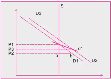
For the HEI that maintains excess demand, this movement is sufficiently large for a given interval of prices, and consequently, the long-term demand curve will be positively inclined in this interval (Figure 1). When the price reaches a suficiently high level, the large shifts in demand stop, and the long term demand becomes negatively sloped. In this case, the tuition rate that maximizes proit (P3) will be below the short term equilibrium price (P4).
Yet, in the case of the HEIs that do not maintain excess demand, the long-term demand curve will be negatively sloped because excess demand does not create a suficiently large shift in the short term (Figure 2).
In analyzing Figure 1, an initial equilibrium in P1 is determined by the D1 demand and supply S. Next, an HEI reduces its price to P2 and creates an excess demand of ab. In
the long term, for this excess demand, the short-term demand curve turns out to be D2, which allows the HEI to charge tuition equal to P3, while maintaining the same excess demand. Note that the excess demand ab generates a shift of demand curve
(from D1 to D2), which implies a higher quantity demanded for P2. In order to maintain both the same excess demand (ab)
and, consequently, D2 as the short-term demand curve, HEI can increase price to P3, reducing the quantity demanded to the previous level (Figure 1). In this step, demand is positively inclined.
If the HEI decides to lower the price below P3, the shift of short-term curve due to an increase in excess demand will be smaller and, as consequence, the long-term demand curve will be negatively inclined (from D2 to D3). In this case, the long--term equilibrium will be in P3, while in the short term (only!) the price P4 maximizes the proits of the HEI.
Following the same sequence in Figure 2, suppose there is an initial equilibrium in P1. A new price P2 would create an excess demand for ab, which would shift the short-term
demand curve to D2. However, in this case, long-term demand (d1) is negatively inclined, since any price higher than P1 generates excess supply. Hence, the equilibrium price is the initial price – P1.
3. EMPIRICAL METHOD
The methodological challenge of this project, given the speciics of this market, is to propose estimation strategies through models of discrete choice and the utilization of instrumental variables that can surpass (at least in part) the econometric dificulties arising from the particularities of the market. These strategies are to:
• redeine the question in order to avoid the problem in which, in the higher education market, the student not only chooses the HEI but is also chosen by the HEI, and so be able to use the Aggregate Logit Model;
• deine the demand for the HEI;
• obtain instrumental variables to correctly estimate the model.
3.1. Econometric model
The methodology used in this paper to estimate the demand for undergraduate business programs in the state of São Paulo is based on the literature of discrete choice applied to the
Figure 2: Long-Term Equilibrium without Demand Excess
estimation of demand in markets with differentiated goods. There is a vast range of references, from the seminal work of Lancaster (1971) and McFadden (1974) to more recent contributions well known in the ield, such as Berry (1994), Berry, Levinsohn and Pakes (1995) (BLP, as they are referred to from here onward) and Nevo (2001). In this paper, we will use the Aggregate Logit Model(3).
This methodology has two important characteristics. The irst of these is that despite being a model of discrete choice, it is based only on aggregated or market data. The second is that the method projects the goods (HEIs, which hereafter refer speciically to São Paulo business schools) in the space of characteristics, and the dimension of this space is the relevant one. In this sense, the problem of dimensionality is resolved when the system of demand equations for differentiated goods is estimated, wherein the price of all goods must appear in every equation.
Before describing this methodology, it is necessary to evaluate if it is adequate for the HEI market. Models of discrete choice assume that the consumer chooses the good or service. This assumption does not match this market, in which the student not only chooses the HEI but also is chosen by the HEI. The fact that a student goes to study at an HEI indicates that there was a matching between them. This interpretation of the process suggests that models of discrete choice are not appropriate for this sector.
In order to avoid this problem and be able to apply a discrete choice model, we redeine the question of interest. Instead of asking the question “at which HEI will students study”, we turn to the question “to which HEI will students apply”. Hence, instead of using the number of registered students as the measure of demand, we use the number of student applications. This approach can be understood in terms of the
student calculating an ex ante utility of studying in a given HEI,
before the decision of the HEI of accepting or not him as its student. This approach allows us to use the traditional methods of discrete choice to analyze this market.
The primary idea behind this method is that students classify HEIs according to their characteristics. We initially assume that the function of ex ante indirect utility that a student has upon
applying to an HEI depends on the HEI quality (qe), the quality
of the students that attend the HEI (e), the price of studying at
the HEI (p) and the dificulty of being accepted to the institution
(sel). We can then write that the utility that the student i has
upon registering at the HEI j is represented as
Uij=U(qej, ej, pj, selj, εij) [1]
where εij is a non-observable characteristic of individual i in
relation to HEI j, for example, if the HEI is close to the residence
of i. We assume that the HEI quality depends on both observable
characteristics (x) and non-observable characteristics (ξ),
then qe=(x,ξ). Assuming that the utility function is linear,
we ind that the utility a student i has on choosing school j is
represented by
uij= αpj + γej + φselj + xjβ + ξj + εij [2]
where α, γ and φ are scalars, β is a vector with dimension K, ξj is an unobserved characteristic of the HEI (j), and εij is a
characteristic idiosyncratic to consumer i in relation to HEI j.
The student chooses between (N+1) options: the N different
HEIs available in the market and the option to not study business (which means studying in a different higher-education program or no higher-education program). The utility of each option for the consumer is represented by the following system:
ui0= x0β + ξ0 + εi0
ui1= αp1 + γe1 + φsel1 + x1β + ξ1 + εi1
... [3]
uiN= αpN + γeN + φselN + xNβ + ξN + εiN
From among the available options, the student chooses the option that grants the best utility. We normalize the utility of the option of not studying business as zero, as is usual. Additionally, we assume that the idiosyncratic characteristic εijis distributed as a type I extreme value distribution, which transforms the
problem into the well known logit(4).Then a consumer chooses
alternative j if uij> uik , k ≠ j, k = 0, 1,... N.
If information about the choice of the consumers were available or if we had microdata, then this study would use the hypothesis of logistically distributed errors to calculate the probability of the consumer choosing each alternative. In that case, the model would be the traditional Multinomial Logit Model. Unfortunately, microdata on consumer choices were not available – only the total number of students that chose a determined HEI. Therefore, a model based on aggregated data is used.
With this aim, we deine:
Aj(x, p, e, sel, ξ; α, β){(εi0, εi1 ... εN) │uij ,
k ≠ j, k = 0, 1,... N} [4]
where x. = (x1,... xN), p. = (p1,... pN), e. = (e1,... eN), sel. = (sel1,... selN) and x. = (x1,... xN) are, respectively, the observable
characteristics, the price vector, the student quality vector, the selectivity vector and the vector of the non-observable characteristics of all N HEIs existing in the market. Group Aj
deines the group of individuals who choose alternative j. It
is important to note that individual i is deined by vector (ei0, ei1 ... eiN). Aggregating all individuals i present in group Aj,
or integrating the distribution e over group Aj, one obtain the
market share of product j:
sj = ∫ f (ε) dε [5]
where f(.) is a density function of the extreme value distribution.
This hypothesis on distribution means that the deined integral in [5] has a closed functional form, represented by the following equation (see Train, 2003, pp. 78 and 79 for the algebraic manipulation that transforms the equation from [5] to [6]):
sj = e
αpj + γej + φselj + xjβ + ξj
[6]
∑keαpk + γej + φselj + xkβ + ξk
Using the log in equation [6], we reach a linear expression of the fraction of consumers that opt for HEI j, which is the
model estimated in this paper:
ln(sj) - ln(so) = αpj + γej + φselj + xjβ + ξj [7]
where sj is the market share of HEI j, and s0 is the market share
of the option to not pursue a higher education or to undertake a program in an area other than business. Two points should be mentioned. Initially, despite the non-linearity of the initial problem, the hypothesis of logit distribution and the aggregation allowed us to reach a linear equation, which simpliies the estimation process.
Secondly, the non-observable characteristic (by the econometrists) of the HEI, x, is the random term of the estimation
model. Observing that this term captures the characteristics of the HEI not included in vector x, it is intuitive to suppose that
this term has a positive correlation with the price, the quality of the students and the selectivity of the HEI. HEIs with better non-observable characteristics in equilibrium charge higher prices, attract better students, and can be more selective. This fact generates a correlation between these variables and the econometric error, resulting in problems of endogeneity for all of them, so instrumental variables are needed to estimate the model. We discuss this issue in the next subsection.
Finally, with respect to the econometric technique, it is necessary then to use those models that permit the use of instrumental variables. We will use the method of two-stage least squares (2SLS).
3.2. Instrumental variables
According to the literature on estimating demand for homogeneous goods, the valid instrument to correct for the endogeneity of the price variable is a set of variables that affect business costs and are unrelated to demand shocks. In theory, the same type of instrument can be utilized in markets with differentiated goods. However, there are rare situations in which cost variables of irms are related to only one differentiated good, without being correlated with all of the market goods. Therefore, another type of instrument should be used.
In literature, there are two possible solutions to this problem. The irst, derived by BLP, uses the exogenous characteristics of the irm’s own product as instruments for themselves and
the sum or average of the rivals irms’ product characteristics as instruments for the price. According to Bertrand’s oligopoly model with differentiated goods, in market equilibrium, the better the quality of the rival goods, the lower the equilibrium price of the irm in question.
The second solution, introduced by Hausman (1996), advocates the use of the same product’s price in another market as an instrument for the price(5). In the problem analyzed here, one HEI is different from another, not having a product brand appearing in different markets, nor two HEIs in different cities. This forces us to opt for the irst solution, in which we use the average of the characteristics of the other HEIs as an instrument for the price.
The quality of enrolled students and HEI selectivity are also endogenous variables. We will use the same group of instrumental variables that we use for price: competitor characteristics, and the age of the HEI. The age must be related to the reputation of the school, the hypothesis being that the older HEIs are more likely to have better reputations.
4. DATASET
As mentioned in the previous section, the model represented by equation [7] will be estimated in this work. We will explain the variables utilized in this estimation, as well as the source of the data.
At the onset, it is important to deine the dependent variable or the market share of the HEIs (variable sj in equation [7]).
This is equal to the ratio between the number of students that want to study at an HEI and the number of potential students in the market where the HEI is located.
To reach the market share denominator, it is necessary to
explain a priori the markets in which the HEI participates. In
the present work, we assume, in a simplifying manner, that each municipality with at least one business program corresponds to a market(6). At the same time, to reach the number of potential consumers of an HEI, the study takes into consideration the fact that the consumer has completed secondary education, is between 18 and 25 years old, and is being confronted with three possibilities: to attend a business program, to attend a higher-education program in another ield or to not attend a higher-education program at all. All of the students who opt for one of these alternatives and who live in the municipality where the HEI is located are part of the HEI’s potential market.
The 2006 Higher Education Census from the Ministério da
Educação e Cultura (MEC – Ministry of Education) provides
number of students in the irst two groups and the participation percentage of the third group, we can estimate the number of potential consumers, which will be the denominator of the market-share formula of the HEI in the municipality. This number is then equal to the ratio between the number of students enrolled in any undergraduate degree (business and others) in the municipality and 0.27.
It is dificult to deine the numerator of the market-share formula of the HEI. As we discussed in the econometric model section, we use the number of students who take the entrance exam for the business program at an HEI(7), in order to avoid the fact that in the education sector not only the students chooses the HEI but also is chosen by it. We are aware that there is a problem with this alternative: many students take various exams, for different HEIs, in the same year. Thus, the average might overestimate the demand for the HEI.
A possible alternative is to use the number of registered students in the HEI business program. The problem with this alternative is that the HEIs that are more selective, that is, that have higher candidate/slots ratios, tend to work with excess demand. As discussed in section 2, they do not adjust the tuition to balance the amount demanded with the amount offered. The reason, as was already discussed, is that in the education sector, the consumer (the student) is also an input in the productive process. The better quality the registered students are, ceteris
paribus, the better the quality of the students educated at the
HEI. This occurs in large part because students can beneit from interacting with the other students, through what is known as the peer effect, and because the quality of the HEI supplies a signal about the quality of the graduate in the job market after completing higher education(8). Moreover, the HEIs with excess demand certainly would have a better market share if they were to have a less rigorous selection process and accept more students. Therefore, the number of registered students as a measure of the numerator for the market-share formula underestimates the demand for the HEIs with higher selectivity. Last but not least, with this alternative, we could not apply the models of discrete choice, as pointed out in the econometric model section. Hence, we do not consider this alternative.
The data of the number of student applicants to each HEI comes from the 2006 Higher Education Census of the MEC.
This study now proceeds to a discussion of the different observable characteristics related to the variable quality of the HEIs that can affect the choice of the student and are used as explanatory variables (variable xj in equation [7]) in the
empirical model. Two variables are related to the quality of the faculty body: the percentage of lecturers with doctorates (perc_doutor) and the percentage of full-time lecturers (perc_ int). These variables are collected from the 2005 Faculty Body Census. At irst, a high percentage of lecturers with doctorates and full-time lecturers might signal the quality of the program; however, the business student certainly is also interested in their lecturers’ business experience, which often competes
with the full-time dedication of a university lecturer. Therefore, whether a superior title means better academic quality in the program (maintaining constant the rest of the variables) is questionable. For example, a lecturer who is also the director of a large company may attract more candidates to a business course than a full-time lecturer with a Ph.D. degree.
Other observable characteristics related to the variable quality of the HEIs used as explanatory variables are the ones related the conditions of the infrastructure offered by the HEI. The models in this paper consider three variables: the quality of the overall physical structure (qual_infra), the quality of the library (qual_libr) and the availability of computers (qual_comp). These three variables are obtained from a socioeconomic survey administered to undergraduate students during the Exame Nacional de Desempenho de Estudantes
(Enade – National Student Performance Exam), carried out by the MEC and compiled at the 2006 Enade Census. The students grade each of these variables and an average score for each of those is obtained. In the case of these three physical--infrastructure variables, the signs of their coeficients are expected to be positive; that is, better infrastructure should correspond to a greater market share.
The authors collected pricing information during the irst semester of 2008. A negative sign for the tuition coeficient is expected.
Every new undergraduate student in business (and in other programs as well) must take an exam that encompass speciic and general knowledge, the Enade. The average score of the students in a given HEI is used in this paper as a proxy for the quality of the student body that the student will ind if he chooses this HEI. This variable comes from the 2006 Enade Census. This variable might signify that the students take into account the effect of their peers (peer effect) in their choice of HEI. Additionally, schools with better students have a better reputation, generating better results for their students in the job market after graduation. In both cases, the higher the Enade score is, the more qualiied the group of students and the higher the demand for the HEI.
The selectivity variable is defined as the number of candidates divided by the number of vacancies. On the one hand, a higher selectivity implies less likelihood that the student will be accepted by the HEI. Hence, we expect that this variable will have a negative effect on the choice of the student. On the other hand, this variable may be seen as another proxy for the quality of the student body. In this regard, the higher Enade score is, the higher is the demand for the HEI. Therefore, the sign of the coeficient of the variable selectivity is unclear from a theoretical point of view.
In terms of the market (municipality) in which the HEI is located – as identiied by the 2006 Higher Education Census – the model includes the Gross Domestic Product (GDP) per
capita of the municipality (GDP-pc) for the year 2007, as
variable (SP) assumes the value one when the HEI is in the market of the capital, the city of Sao Paulo, and zero otherwise. As the density of business programs in relation to the total population is smaller in the capital than in other cities, an inferior market share is expected in the capital.
Our sample contains 298 observations of HEIs located in 130 municipalities (or markets) in Sao Paulo state. As previously mentioned, each market is deined as a municipality.
Table 1 shows the distribution of programs in the different markets. In 83 markets (municipalities), or in 63% of markets, there is only one undergraduate business program. Two HEIs share students in 25 markets, and 97 programs are distributed through 21 markets, each containing between 3 and 11 competitors. Additionally, the principal market is certainly the municipality of Sao Paulo, where there is a concentration of 22.8% (n=68) of all programs in the state.
Table 2 presents a statistical summary of the variables used in the analysis, with the average and standard deviation of each one. The average of the dependent variable, i.e., the market share, is equal to 6.9% once the total market includes all of the individuals of university age who have completed
secondary school, whether enrolled in a business program or not. The HEIs are, on average, 9.2 years old, and practically all offer a bachelor’s program rather than a technical program.
The average Enade score of the registered students is equal to 39.5 (on a scale of 0 to 100). Considering only the 20 programs with the highest candidate/vacancy ratios, the Enade average rises to 44.6.
The average tuition is equal to R$ 506,85 (or US$ 318), and the municipalities’ average GDP per capita is equal to
R$ 28.750,95 (or US$ 18,082). Additionally, among the HEIs analyzed, the average percentage of lecturers with doctorates and full-time lecturers are, respectively, 8.5% and 12.5%.
Table 3 shows the distribution of the average scores of the variables related to the conditions of the infrastructure: the quality of the overall physical infrastructure, the library, and computer availability. The second, third and fourth columns present the number of programs with evaluation, respectively, “worse than average by one standard deviation (sd)”, “average ± one sd”, and “better than average by one sd”.
Finally, Figure 3 summarizes the data sources.
5. EMPIRICAL ANALYSIS
In this section, we show and discuss the empirical results. In the irst part, various estimates will be presented, which vary according to the explanatory variables used. Here, we aim to explain which factors are considered by students when choosing a HEI. In the second part, using the coeficients estimated, the HEI’s investment in excess demand is calculated.
5.1. Results of the regressions
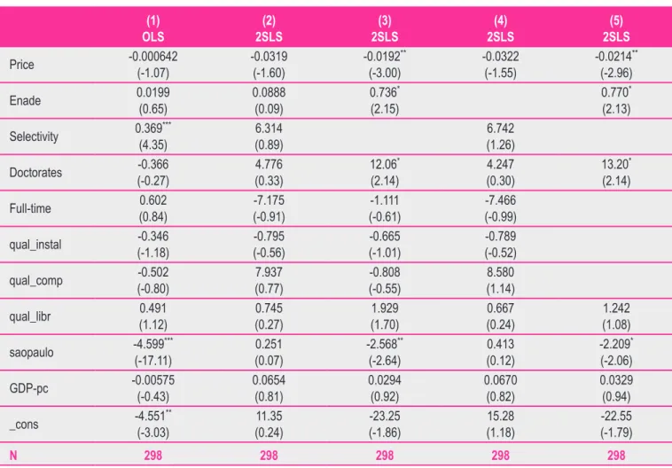
Table 4 shows the results of the different estimation models. Model (1) is estimated via OLS. Models (2) through (5) are estimates with instrumental variables (IVs) for the price, Enade score and selectivity via 2SLS.
As mentioned in the previous section, OLS is not the indicated method in this case, but we present the result of this estimate to highlight the effect of the instrumental variables. The comparison between model (1) and the others allows us to identify a substantial difference when we use IVs for the estimate of the models. In particular, the coeficients of the variables price, Enade and selectivity change substantially when the 2SLS method is employed.
For models (2) through (5), the IVs used is the average values of the other HEIs (the rivals) for the following characteristics: the percentage of lecturers with doctorates (ivdoc), the quality of the infrastructure (ivinstal), the quality of the computers (ivcomp), the quality of the library (ivbibl) and the percentage of full-time lecturers (ivintegr). Moreover, we use the age of the HEI itself as a measure of its reputation, which should have a direct impact on students’ choices and Enade scores. We observe in the correlation of variables in Table 1
HEI and Markets
Number of HEI Number of Markets Total
1 83 83
2 25 50
3 to 11 21 97
68 1 68
Total 130 298
Table 2
Statistical Summary
Variable Average Standard
Deviation
Market Share (%) 6.9 11.2
Enade Score (0-100) 39.5 4.3
Price (R$) 506,85 249.2
Lecturers with Doctorates (%) 8.5 9.3 Full-time Lecturers (%) 12.5 15.1 GDP per capita (R$) 28.750,95 18.200,1
Age 9.2 12.2
Table 3
Distribution of Quality of Physical Infrastructure
Variable Worse than average by one
standard deviation
Average ± one standard deviation
Better than average by one
standard deviation Total
qual_infra 48 201 49 298
qual_comp 42 204 52 298
qual_libr 46 206 46 298
Variable Source
Population Population Census – Brazilian Bureau of Statistics (IBGE) Applicants and enrolled students and by IES, course 2006 Higher Education Census – Ministry of Education (MEC) Percentage of lecturers with doctorates and full-time lecturers 2005 Faculty Body Census – Ministry of Education (MEC) Quality of computers, infrastructure and library 2006 ENADE (National Student Performance Exam) – Census Average HEI quality 2007 ENADE (National Student Performance Exam) – Census
Per capita GDP in 2007 IPEADATA
Name and location of a HEI 2006 Higher Education Census – Ministry of Education (MEC)
HEI Tuition Collected by the authors in 2008
Figure 3: Summary of Data Sources
Table 5 that the Enade scores as well as the price of the HEI show a correlation of around 0.3 with the age of the institution.
The results of the irst stage of the models (2) through (4), which contains all of the variables, are presented in Appendix 1. Importantly, some of the IVs are signiicant and exhibit the expected sign, coniguring instruments that present a signiicant (conditional) correlation with the endogenous variable.
Tuition, Enade scores, and selectivity are all endogenous variables, and they represent the market equilibrium of the HEI. Some dificulties arise with this fact. First, at equilibrium, these variables are positively correlated: better HEIs charge a higher tuition, are more selective, and attract better students, implying a positive correlation between these three variables (see Table 5). Secondly, as discussed, the instruments used in the identiication of the model are made up of the exogenous characteristics of the HEIs that determine the market equilibrium and, therefore, are the same for these three variables. In contrast, BLP uses the group of instruments to identify only one endogenous variable, instead of three in this case.
All of these factors complicate the identiication of the effect of these three variables, as can be observed in model (2) of Table 4. This speciication includes all of the explanatory variables, including tuition, Enade scores, and selectivity. None of these is signiicant in this speciication. The positive correlation between them complicates the correct identiication
of the parameters. To avoid this problem, we estimate the model with only Enade (models (3) and (5)) or selectivity (model 4) as the explanatory variable, apart from tuition.
The only difference between models (3) and (5) is the fact that some control variables (full-time, qual_instal and qual_comp) are excluded in the last model. The results of models (3) and (5), which exclude selectivity, are similar to each other. The coeficients of the price variable are approximately -0.02, and those of the Enade score variable are approximately 0.74. The percentage of lecturers with doctorate degrees is also statistically signiicant, with a coeficient close to 13. The coeficients of the other variables are also robust compared to the different speciications. The results in these models suggest the importance of the price variable for student choice.
Table 5
Correlation
MS Price Enade Selectiv Doctor Full-Time qual_inst qual_comp qual_libr Age
Ms 1.00
Price -0.21 1.00
Enade -0.14 0.60 1.00
Selectivity 0.04 0.39 0.32 1.00
Doctor -0.11 0.51 0.42 0.36 1.00
Full-Time -0.12 0.16 0.22 0.23 0.27 1.00
qual_instal -0.03 0.17 0.22 0.06 0.12 0.14 1.00
qual_comp 0.01 0.27 0.30 0.04 0.24 0.15 0.58 1.00
qual_libr 0.06 0.24 0.27 0.13 0.13 0.18 0.58 0.60 1.00
Age -0.14 0.25 0.28 0.18 0.23 0.24 0.00 0.14 0.07 1.00
Table 4
Econometric Results
(1) OLS
(2) 2SLS
(3) 2SLS
(4) 2SLS
(5) 2SLS
Price -0.000642
(-1.07) -0.0319(-1.60) -0.0192 **
(-3.00) -0.0322(-1.55) -0.0214 ** (-2.96)
Enade 0.0199(0.65) 0.0888(0.09) 0.736
*
(2.15) 0.770
* (2.13) Selectivity 0.369(4.35)*** (0.89)6.314 (1.26)6.742
Doctorates -0.366
(-0.27) (0.33)4.776 12.06
*
(2.14) (0.30)4.247 13.20
* (2.14) Full-time 0.602(0.84) (-0.91)-7.175 (-0.61)-1.111 (-0.99)-7.466
qual_instal (-1.18)-0.346 (-0.56)-0.795 (-1.01)-0.665 (-0.52)-0.789
qual_comp (-0.80)-0.502 (0.77)7.937 (-0.55)-0.808 (1.14)8.580
qual_libr 0.491(1.12) (0.27)0.745 (1.70)1.929 (0.24)0.667 1.242(1.08)
saopaulo -4.599(-17.11)*** (0.07)0.251 -2.568(-2.64)** (0.12)0.413 -2.209(-2.06)*
GDP-pc -0.00575(-0.43) 0.0654(0.81) 0.0294(0.92) 0.0670(0.82) 0.0329(0.94)
_cons -4.551(-3.03)** (0.24)11.35 (-1.86)-23.25 (1.18)15.28 -22.55(-1.79)
N 298 298 298 298 298
quality of the student body on the choice of the applicant has to do with what the literature calls the peer effect. This effect consists of the positive externality that qualiied colleagues have on the learning process. In other words, studying and living with intelligent and studious individuals contributes to the student’s ability to learn. For this reason, the quality of the students in the HEI affects the decision of the applicants(11). With the available data, it is not possible to deine which of the alternatives better explains the decision to take the entrance exam; we limit ourselves to the conclusion that students have a preference for better peers.
In model (4), in comparison with model (2), we exclude the variable Enade. The variable “selectivity” is not statistically different from zero. As we mentioned before, this variable captures two effects. On the one hand, a higher selectivity implies less likelihood that the student will be accepted by the HEI and a negative sign is expected. On the other hand, this variable is a proxy for the quality of the student body, and a positive sign is expected. The empirical result suggests that the net effect is zero.
In Table 4, we still observe that the percentage of full-time lecturers shows is not signiicant in all models, similar to the coeficients for computer access and infrastructure quality. Business students might prefer to take classes with lecturers who are professionals in the market, and therefore part-time at the HEI, rather than with lecturers with a full time academic profession. This may explain the non-significance of the percentage of full-time lecturers in the students’ choice.
The percentage of lecturers with doctorates, in contrast, seems to be a relevant variable to the student decision-making process. This variable has a positive value and is statistically signiicant in all of the estimate speciications via IVs that do not include selectivity. Taken together, the results obtained by the characteristics of the faculty – the percentage of lecturers with doctorates and the percentage of full-time lecturers – indicates that students take into account faculty quality, but that lecturers do not need to be academics in the traditional sense, i.e., dedicated solely to research and teaching.
The quality variables of the HEI are not signiicant. A possible cause for this is the high correlation that exists between them, close to 0.6 (Table 5). For this reason, we remove infrastructure quality and computer access from the speciication (5) of the model, but the results do not change substantially. The quality of the library coeficient continues to be non-signiicant in this speciication.
Aside from the variables mentioned, we include controls for characteristics of the counties: GDP per capita and a
dummy for the city of São Paulo. We believe that the São Paulo dummy makes the value of the price coeficient more accurate. Without this differentiation, the regression might overestimate the impact of price because the correlation between lower tuition and greater participation in the market might be partially explained not by a causal relationship but
by the fact that these characteristics are typical in the markets of smaller cities. Yet, the programs in the city of San Paulo, a city with a higher cost of living, tend to have smaller market shares, since the market-share denominator is the number of potential applicants, which is enormous for the São Paulo’s market. Therefore, the higher prices of the São Paulo programs and their smaller market share might intensify the impact of prices on the market-share, if the regression were not to include a dummy for the city of São Paulo. The interpretation seems clear: the programs in the city of São Paulo tend to present a market share smaller than the others and are, on average, more expensive (R$ 663,9 or US$ 417 in the capital versus R$
460,3 or US$ 289 in the other cities). Therefore, if we had not controlled for location (capital versus countryside), we would
have created an overestimation of the importance of the price in the determination of the market share.
5.2. Estimation of the “investment” in excess demand
According to the results presented in the prior section, one can estimate the total volume of revenue that a speciic HEI gives up by maintaining a lower tuition in order to generate excess demand and, therefore, selectivity of the applicants for the business program. The procedure is simple. Using the price coeficient estimated in the previous section, one can calculate the necessary price increase that would reduce the HEI market share in order to eliminate the excess demand. In other words, the price increase that would make the number of applicants equal to the number of offered slots. The amount of revenues that the HEI gives up is equal to the difference between the price that would eliminate the excess demand and the actual price charged multiplied by the number of slots available.
Before presenting the results, a methodological procedure deserves mention. This estimation should be made only for the HEI that has a number of offered spaces lower than the number of applicants, which is a condition necessary but not suficient for the characterization of excess demand. Furthermore, the applicants should ill all of the spaces because some institutions present a number of applicants greater than the number of slots but without all the slots being illed, which does not allow us to identify excess demand. Therefore, it is important that there are no unilled slots. However, in some cases, the HEIs present an applicant/vacancy ratio much greater than one, but only one or two spaces are not illed. Clearly, in this case, the unilled space is not a consequence of demand scarcity for the program but simply an operational question or a registration cancellation. For this reason, we considered programs with a number of applicants greater than the total number of vacancies and with at least 98% of the slots occupied.
signiicant coeficients and all control variables are present. The values correspond to the annual revenue that the HEI gives up in the year 2006 with regard to the irst-year class.
There are 39 HEIs with excess demand, and the value of the “lost” revenue is presented for each HEI in a growth curve. In model 3, 39 HEIs in the state of Sao Paulo gives up, in the short term, a total of R$ 5.499 million (or US$ 3,458 million) per year by “investing” in the selectivity of their students. Considering the 39 HEIs with excess demand, this amount corresponds to 7.6% of the total revenue coming from a freshman class.
6. CONCLUSION
This article analyzes the private higher education sector and attempts to explain and quantify some particularities of this sector, such as the strategy of some institutions to maintain permanent excess demand and the strong segmentation that exists in this market. To achieve this objective, various peculiarities in this sector had to be taken into account in the analysis, requiring speciic theoretical and empirical treatment, which we explain throughout the paper.
On the empirical part, there are two aspects that make the analysis more complex. First, the HEI’s market is a matching
market, which consists of students choosing the HEI as well as the HEI selecting the students. To avoid this problem, we changed the student’s question from “at which HEI to study”
to “at which HEI to apply.” Instead of using the number of registered students as a measure of demand, we use the number of applicants in the selection process. This avoids the problem of the matchingmarket because the application precedes the
HEI’s selection process.
The second difficulty results from the fact that some variables that determine the decision of the student are endogenous, such as tuition, quality of the student body and the HEI’s selectivity. These variables are determined by the market equilibrium, so that there is no causal relationship between them and the irm’s market share. We use the solution proposed by BLP, using the characteristics of the competitors, in addition to the age of the HEI itself, as instruments for the endogenous variables of the model.
Using data from all business-administration programs in the state of São Paulo, the study shows that the most relevant factors for student choice are the tuition charged by the institution and the quality of the lecturers and students. The other characteristics, such as the quality of the infrastructure or computer access, are shown to be insigniicant. In a general way, we found evidence that the tuition and quality of both lecturers and the student body deine an institution and its position in the market.
mentioned, the empirical strategy is to measure the revenue amount that HEIs give up to be able to select the best students. As far as we know, estimating the investment on student quality – which means higher peer effect and better graduates – by using the methodology proposed here, is quite new.
The results show that, among the small group of 39 HEIs with positive investment, the total amount is signiicant only for very few of them. Instead of dividing the business courses into two groups – with positive and zero investment on student selection – the results suggest the existence of three groups: (1) HEIs with no investment; (2) HEIs with very small investment; and (3) HEIs with signiicant investment. It is hard to think of HEIs of the second group as institutions really willing to invest on student quality; rather the excess demand seems to be occasional. Therefore, of the total of 298 courses, only three or four institutions – depending on the criterion chosen – invest on the quality of their students.
It is worth examining the possible strategies for those courses of the irst and second groups that do not invest on selection. One strategy is to reduce costs as much as possible so that they can attract students by reducing prices. An alternative strategy would be to invest on both physical resources (modern labs and equipments) and hiring good lecturers. However, in
this market, as mentioned, the demanders (students) can be understood as input and complementary to physical resources and lecturers. As HEIs of the irst and second groups do not invest on student quality, one should expect that the return of their investment on any other input will be lower than the return of the investment made by a selective HEI.
This scenario suggests that the market of business courses in Brazil is, in fact, composed by only two types of HEIs: those that invest zero or little on selection – more than 95% – and compete by reducing costs and prices, with little attention on quality; and those – three or four institutions – that invest on quality and reputation.
Surely, the present study does not attempt to exhaust the subject; rather, the idea is to open topics for further research that may answer important questions that were not central to the objective of this article. The demand estimated in the irst section, using cross-sectional data, with an observation on each institution, corresponds to what we consider throughout the article to be short-term demand. A new investigation that estimated the size of external diffusion (network externality) in the higher-education sector would be extremely valuable. Additionally, alternative solutions from the point of view of econometric methodology might also be tested.
(1) The exchange rate used in this paper is R$ 1,59 to buy one dollar, of June 14th, 2011.
(2) 24.1% of the HEIs in the country are located in São Paulo, and the ield of business is the largest in terms of number of programs (7.6% of the total) and number of registered students (13.9% of total students).
(3) A substantial part of this literature is devoted to overcome the Independence of Irrelevant Alternatives (IIA) feature of the logit model [see Train (2003) for a discussion about IIA]. It is not a source of concern here, since we are not interested in estimating cross--elasticities or substitution patterns among HEIs.
(4) It is worth noting that what is relevant is the utility difference among the schools. The random variable formed by the difference between two random variables with extreme value distribution follows a logistic distribution (see Train, 2003).
(5) For a discussion of the pros and cons of each kind of instrument, see Nevo (2001).
(6) An alternative would be to deine the market in terms of economic regions of different municipalities.
However, a certain amount of arbitrariness would be necessary to deine these alternative market borders. Another alternative would be to consider the city of São Paulo as more than one market because of its size. Again, it would be dificult to deine the boundaries of this market. Next, we will propose models that seek to capture the speciicity of the São Paulo market.
(7) In Brazil, all applicants to a given HEI must take an entrance exam.
(8) See Winston and Zimmerman (2003) for a summary of the literature on the peer effect and MacLeod and Urquiola (2009) on the effect of the reputation of the school on the quality of the students.
(9) See <www.ipeadata.gov.br>.
(10) MacLeod and Urquiola (2009) formalize this argument.
(11) Epple and Romano (1998) develop a model of competition between schools, where the peer effect is the key factor in the division of schools by quality.
N
O
T
Becker, G. (1991). A note on restaurant pricing and other examples of social inluence on price. The Journal of Political Economy, 99, pp.1109-1116.
DOI: 10.1086/261791
Belzil, C., & Hansen, J. (2002). Unobserved ability and the return to schooling. Econometrica, 70, pp. 2075-2091. DOI: 10.1111/1468-0262.00365
Berry, S. (1994). Estimating discrete-choice models of product differentiation. Rand Journal of Economics, 25, pp.242-262.
DOI: 10.2307/2555829
Berry, S., Levinsohn, J., & Pakes, A. (1995). Automobile prices in the market equilibrium. Econometrica, 6, pp.841-890.
DOI: 10.2307/2171802
Bishop, J. (1977). The effect of public policies on the demand for education. Journal of Human Resources. 12, pp. 285-307.
DOI: 10.2307/145492
Chowdry, H., Crawford, C., Dearden, L., Goodman, A., & Vignoles, A. (2010). Widening participation in higher education: Analysis using linked administrative data. IZA Discussion Papers 4991. Institute for the Study of Labor (IZA).
Ehrenberg, R. (2004). Econometric studies of higher education. Journal of Econometrics, 121, pp.19-37. DOI: 10.1016/j.jeconom.2003.10.008
Epple, D., & Romano, R. (1998). Competition between private and public schools, vouchers and peer-group effects. American Economic Review, 88, pp.33-62.
Flannery, D., & O’Donoghue, C. (2013). The demand for higher education: a static structural approach accounting for individual heterogeneity and nesting patterns. Economics of Education Review, 34, pp. 243-257.
DOI: 10.1016/j.econedurev.2012.12.001
Frenette, M. (2009). Do universities beneit local youth? Evidence from the creation of new universities. Economics of Education Review, 28, pp.318-328.
DOI: 10.1016/j.econedurev.2008.04.004
Gallego, F., & Hernando, A. (2008). On the determinants and implications of school choice: semi-structural simulations
for Chile. Journal of the Latin American and Caribbean Economic Association,9, pp.197-229.
Hartog, J., & Dias-Serrano, L. (2007). Earnings risk and demand for higher education: A cross-section test for Spain. Journal of Applied Economics, 0, pp. 1-28.
Hausman, J. (1996). Valuation of new goods under perfect and imperfect competition. In T. Bresnahan & R. Gordon (Eds.), The Economics of New Goods, Studies in Income and Wealth, Vol. 58, Chicago: NBER.
Kelchtermans, S., Verboven, F. (2009). Reducing product diversity in higher education. Proceedings of the 36 EARIE; Ljubljana, Slovenia; 3-5 September 2009.
Lancaster, K. (1971). Consumer demand: A new approach. New York: Columbia University Press.
Long, B. (2004). How have college decisions changed over time? An application of the conditional logistic choice model. Journal of Econometrics. 121, pp. 271-296.
DOI: 10.1016/j.jeconom.2003.10.004
McFadden, D. (1974). Conditional logit analysis of qualitative choice behavior. In P. Zaremba (Ed.), Frontier of econometrics. New York: Academic Press.
MacLeod, W., & Urquiola M. (2009). Anti-lemons: School reputation and educational quality. NBER Working Papers # 15112.
Monks, J., & Ehrenberg, R. (1999). The impact of U.S. News & World Report College rankings on admissions outcomes and pricing policies at selective private institutions. NBER Working Paper # 7227.
Nevo, A. (2001). Measuring market power in the ready-to-eat cereal industry. Econometrica, 69, pp.307-342.
DOI: 10.1111/1468-0262.00194
Spiess, C., & Wrohlich, K. (2010). Does distance determine who attends a university in Germany? Economics of Education Review, 29, 470-479.
DOI: 10.1016/j.econedurev.2009.10.009
Train, K. (2003). Discrete choice methods with simulation. Cambridge, UK: Cambridge University Press.
DOI: 10.1017/CBO9780511753930
Winston, G., & Zimmerman, D. (2003). Peer effects in higher education. NBER Working Paper #9501.
Permanent demand excess as business strategy: an analysis of the Brazilian higher-education market
Many Higher Education Institutions (HEIs) establish tuition below the equilibrium price to generate permanent de
-mand excess. This paper irst adapts Becker’s (1991) theory to understand why the HEIs price in this way. The fact that students are both consumers and inputs on the education production process gives rise to a market equilibrium where some irms have excess demand and charge high prices, and others charge low prices and have empty seats.
R
EF
ER
EN
C
ES
A
B
ST
R
A
C
Second, the paper analyzes this equilibrium empirically. We estimated the demand for undergraduate courses in Business Administration in the State of São Paulo. The results show that tuition, quality of incoming students and percentage of lecturers holding doctorates degrees are the determining factors of students’ choice. Since the student quality determines the demand for a HEI, it is calculated what the value is for a HEI to get better students; that is the total revenue that each HEI gives up to guarantee excess demand. Regarding the “investment” in selectivity, 39 HEIs in São Paulo give up a combined R$ 5 million (or US$ 3.14 million) in revenue per year per freshman class, which means 7.6% of the revenue coming from a freshman class.
Keywords: higher education, market segmentation, excess demand.
Exceso de demanda permanente como estrategia de mercado: un análisis del mercado brasileño de educación superior
Muchas instituciones de educación superior (IES) establecen precios para sus cursos más bajos que el precio de equi
-librio de mercado con el in de crear exceso de demanda. Inicialmente, en este estudio, se adapta la teoría de Becker (1991) para entender ese comportamiento de las IES. El hecho de que los estudiantes sean a la vez consumidores e insumo en la función de producción de educación lleva a un equilibrio de mercado, en que algunas IES determinan altos precios y trabajan con exceso de demanda, y otras colocan precios bajos y siguen con plazas no ocupadas. Se analiza dicho equilibrio empíricamente y se estima la demanda por cursos de Administración de Empresas en el es
-tado de São Paulo. Los resul-tados indican que el precio, la calidad de los estudiantes ingresantes y el porcentaje de profesores que poseen doctorado son los factores que determinan cuál IES los estudiantes escogerán. Así, dado que la calidad de los estudiantes determina la demanda por una IES, se calcula el valor, para una IES, de tener mejores estudiantes. Dicho valor es igual a los ingresos que deja de recibir para mantener exceso de demanda y selección de estudiantes. Con relación a la inversión en selección de estudiantes, 39 IES en el estado de São Paulo dejaron de recibir ingresos de aproximadamente cinco millones de reales al año por grupo de estudiantes ingresantes, lo que equivale al 7,6% de los ingresos de un grupo de ingresantes.
Palabras clave: enseñanza superior, segmentación de mercado, efecto de pares.
A
B
ST
R
A
C
T
R
ESU
APPENDIX I
First-Stage Regressions
ivregress 2sls y (price Enade score selectivity = ivdoc ivintegr ivinstal ivcomp ivbibl idade) lecturers with doctorates full-time lecturers qual _instal qual_comp qual_libr São Paulo GDP, irst.
Number of obs = 298 F(13, 284) = 17.13
Prob > F = 0 R-squared = 0.4394 Adj R-squared = 0.4138
Root MSE = 190.7078
Price Coef. Std. Err. t P>t [95% Conf. Interval]
doctorate 1008.407 134.3834 7.5 0.000 743.8932 1272.921
full-time -54.1632 80.72751 -0.67 0.503 -213.0634 104.737
qual_instal -27.56862 32.68935 -0.84 0.400 -91.91277 36.77554
qual_comp 76.03494 67.64821 1.12 0.262 -57.12057 209.1904
qual_libr 135.4646 47.90007 2.83 0.005 41.18042 229.7488
saopaulo -707.8994 362.8459 -1.95 0.052 -1422.108 6.30914
GDP 2.02062 1.47984 1.37 0.173 -0.8922256 4.933466
ivdoc -274.127 94.74874 -2.89 0.004 -460.6259 -87.6281
ivintegr 68.2894 58.28421 1.17 0.242 -46.43444 183.0132
ivinstal -46.37654 25.04962 -1.85 0.065 -95.68302 2.929934
ivcomp 56.59547 41.48354 1.36 0.174 -25.05873 138.2497
ivbibl -22.91079 35.69463 -0.64 0.521 -93.17039 47.34881
idade 1.587884 0.996742 1.59 0.112 -0.3740543 3.549823
_cons 621.7086 91.41559 6.8 0.000 441.7705 801.6467
Number of obs = 298 F(13, 284) = 10.13
Prob > F = 0 R-squared = 0.3204 Adj R-squared = 0.2893
Enade Coef. Std. Err. t P>t [95% Conf. Interval]
doctorate 12.09247 2.567086 4.71 0.000 7.039544 17.1454
full-time 1.740024 1.542114 1.13 0.260 -1.295399 4.775447
qual_instal 0.0823146 0.624455 0.13 0.895 -1.146833 1.311462
qual_comp 1.894934 1.292264 1.47 0.144 -0.6486966 4.438564
qual_libr 1.982027 0.915021 2.17 0.031 0.1809435 3.78311
Saopaulo 2.256302 6.931338 0.33 0.745 -11.38701 15.89962
GDP 0.0204556 0.028269 0.72 0.470 -0.0351876 0.076099
ivdoc -5.75277 1.809957 -3.18 0.002 -9.315403 -2.19014
ivintegr 0.7415933 1.113386 0.67 0.506 -1.449942 2.933129
ivinstal -0.5083176 0.478516 -1.06 0.289 -1.450205 0.433569
ivcomp -0.3936111 0.792448 -0.5 0.620 -1.953427 1.166205
ivbibl 0.5855984 0.681864 0.86 0.391 -0.7565499 1.927747
idade 0.040099 0.019041 2.11 0.036 0.0026207 0.077577
_cons 43.66687 1.746285 25.01 0.000 40.22956 47.10417
Number of obs = 298 F(13, 284) = 5.1
Prob > F = 0 R-squared = 0.1892 Adj R-squared = 0.1521
Root MSE = 1.2611
Selectivity Coef. Std. Err. t P>t [95% Conf. Interval]
doctorate 4.300412 0.888617 4.84 0.000 2.5513 6.049524
full-time 0.9045524 0.533815 1.69 0.091 -0.1461836 1.955288
qual_instal -0.03066 0.21616 -0.14 0.887 -0.4561392 0.394819
qual_comp -0.9940431 0.447328 -2.22 0.027 -1.874541 -0.11355
qual_libr 0.6006139 0.316742 1.9 0.059 -0.0228455 1.224073
Saopaulo -1.602265 2.399338 -0.67 0.505 -6.325007 3.120478
GDP 0.0016438 0.009786 0.17 0.867 -0.0176175 0.020905
ivdoc -1.240264 0.626531 -1.98 0.049 -2.473497 -0.00703
ivintegr -0.0840831 0.385408 -0.22 0.827 -0.8427007 0.674535
ivinstal -0.171523 0.165642 -1.04 0.301 -0.4975647 0.154519
ivcomp 0.2393273 0.274312 0.87 0.384 -0.3006156 0.77927
ivbibl -0.1370188 0.236033 -0.58 0.562 -0.6016142 0.327577
idade 0.008284 0.006591 1.26 0.210 -0.0046894 0.021257