doi: 10.1590/0101-7438.2017.037.01.0173
USE OF STOCHASTIC VOLATILITY MODELS IN THE VARIABILITY OF PASSENGERS AND CARGO TRANSPORT IN SOME
AIRPORTS IN S ˜AO PAULO STATE, BRAZIL
Jorge Alberto Achcar
1,3, Luiz Rodrigo Bonette
1and Walther Azzolini Junior
1,2*Received March 17, 2016 / Accepted March 16, 2017
ABSTRACT.The proposed study is related to the identification of important factors that determine the feasibility of regional airport hubs in S˜ao Paulo State, Brazil. This way, new perspectives are created to map airports in this region based on economic criteria of operations and volumes. The study is based on statis-tical data analysis of time series related to operations and volume of passengers and cargo transport data sets during a fixed period of time. Stochastic volatility models are applied for the logarithmic transformed counting data set considering the four largest airports selected from a group of 32 airports in the S˜ao Paulo State chosen by their importance in the amount of passenger and cargo for the period ranging from the year 2008 to the year 2014. This study is a new approach in the analysis of air transport time series.
Keywords: stochastic volatility models, hubs, passenger and cargo air transport, Bayesian methods, time series.
1 INTRODUCTION
The literature presents many studies on hub air transport network associated with the transport of passengers and hub location problems, so-called p-hubs and few studies associated with the transport of cargo. The present study’s goal is related to the association of some important eco-nomic factors to the monthly counting of passengers and volume of air cargo transported in some important airports located in a industrialized region of Brazil.
This way, new statistical modeling is proposed in the analysis of airport operations related to some economic covariates. For this goal, it is proposed the use of stochastic volatility models considering the logarithm of the counting data for the analysis of data sets related to the four more
*Corresponding author.
1UNIARA – Universidade de Araraquara, 14801-340 Araraquara, SP, Brasil. E-mails: [email protected]; [email protected]
important airports selected from 32 airports located in S˜ao Paulo State obtained from statistical handling reports of S˜ao Paulo Airway Department (DAESP-http://www.daesp.sp.gov. br/), Brazil, an office linked to the air transport of S˜ao Paulo State.
Observe that standard counting models based on regression Poisson models (generalized linear models, see for example, Nelder & Wedderburn, 1972) could also be used in the analysis of the data set, but the use of stochastic volatility models in the logarithm scale of the counting data gives more flexibility to simultaneously model of the mean and variance (volatility) of the time series.
The use of stochastic volatility models is becoming very popular in the analysis of financial time series, but is rarely used to analyze time series in transport applications.
The seasonality and volatility of passenger and air cargo transportation in regional hubs are studied in terms of airport economic importance using statistical volatility models that link the dependence of observed economic factors (covariates) to the responses (passenger and cargo counting) and also non-observed factors linked to the volatilities. From the 32 airports available in the DAESP report, we consider the four more important airports in our study which gives a good view of the sector.
The customization of p-hub designs for air loads (Morrel & Pilon, 1999) and location distribution of air cargo systems due to transient hubs are described by Kara & Tansel (2001). Lin et al. (2003) study the indirect connections to large postal cargo hubs networks in general and the multiple use of aircraft capabilities to consolidate center-to-center hubs and the development of flow models to generate improvements in strategic mapping of hubs networks air cargo. Gardiner & Ison (2005), Gardiner & Humphreys (2005), Gardiner & Ison (2008) quantifies the importance of an individual airport by the concept of “airport hierarchy” (primary hubs, secondary hubs, tertiary hubs). Alumur et al. (2007) emphasize the need to determine potential flows hubs at airports by the criterion of the analysis of volumes of cargo operations in a multi-modal and hierarchical network.
Several studies emphasize issues related to the capacity of an airport (see for example, Smilowitz & Daganzo, 2007; Tan & Kara, 2007; Scholz & Cossel, 2001; Petersen, 2007; Bartodziej et al., 2009; Leung et al., 2009; Li et al., 2009; Wang & Kao, 2008; Amaruchkul & Lorchira-choonhkul, 2011).
• The growth of air freight tonnages changing the relationship between passengers and cargo has become a significant source of revenue for airlines and airports;
• The importance of individual airports on a network usually assessed by measures linked to passenger counting, cargo and operating numbers;
• The combined passenger and cargo services are operated in the major airlines.
Scholz & Cosel (2011), Onghena (2011) and Heinicke (2006, 2007) point out that the literature is scarce on this subject and this type of research has been mostly focused on integration between airlines and not in the integration of hub-and-spoke networks. Some important studies on the subject are also introduced by other authors (Grosso & Shepherd, 2011; Alumur & Yaman, 2012; Bowen, 2012; Oktal & ¨Ozger, 2013; Lakew & Tok, 2015). Feng et al. (2015) describe that freight transport is more complex than passenger transport since the freight transport involves more professionals, more sophisticated processes combining volume, varying priority services, integration strategies and various itineraries in a transmission system (see also, Huang & Lu, 2015).
The paper is prepared as follows: in section 2, it is presented the goals of the research and the data set; in section 3, it is presented the statistical analysis of the S˜ao Paulo State airport data (cargo and passengers) using volatility stochastic models; finally, in section 4, it is presented some concluding remarks.
2 DESCRIPTION OF THE GOALS AND THE DATA SET
A study to determine strategic hubs associated with the flux of passengers and the volume of air cargo transported in a region is a starting point for research still scarce in Brazil where this approach could generate important strategic contributions to air transport networks and impacts on the local and regional economy of these airports. The statistical method used in this work seeks to analyze the temporal time series data obtained from statistical reports of DAESP for the years period ranging from 2008 to 2014 extracted from a set of 10,572 observations formed by 32 airports, two response variables (monthly counting of passengers and cargo) associated with the economic covariates dollar rate and unemployment rate obtained from the economic office ACSP (http://www.acsp.com.br/).
Figure 1– Time series for passenger/cargo counts for the airports of Ribeir˜ao Preto, S˜ao Jos´e do Rio Preto, Bauru/Arealva and Presidente Prudente.
From Figure 1, it is observed that:
• Apparently, the number of passengers increases over time for all airports; then after a given change point time there is a small decreasing.
The main goals of the study are given by:
• For the statistical analysis of the data set, it is proposed the use of a stochastic volatility model for the logarithm of the counting data, which gives a great flexibility to simulta-neously model the mean and the variance (volatility) of the time series, that is, a new statistical approach to analyze transportation data.
• The mean of the time series is modeled by a multiple linear regression model relating the mean to the selected covariates (dollar exchange, monthly unemployment rate, years and months) for the two responses (count passenger/cargo) considered in the logarithm scale.
• The variances of the time series are modeled assuming volatility stochastic models, which incorporate seasonal effects given by latent or non-observed variables.
3 STATISTICAL ANALYSIS OF THE S ˜AO PAULO STATE AIRPORT DATA USING STOCHASTIC VOLATILITY MODELS
To study the relationship between the variables and to find the most important factors affecting the variability of passenger count/load in the period from January 1, 2008 to December 31, 2014, we consider a statistical analysis assuming multiple linear regression models relating the average response in logarithmic scale (passenger and cargo counting) to the monthly covariates (dollar exchange, monthly unemployment rate, years and months) and simultaneously modeling the variances of the responses assuming volatility stochastic models.
3.1 Use of stochastic volatility models under a Bayesian approach
Stochastic volatility models (SV) has been extensively used to analyze financial time series (see Danielsson, 1994; Yu, 2002) as a powerful alternative for existing auto-regressive models such as ARCH (autoregressive conditional heteroscedastic) introduced by Engle (1982) and the gen-eralized autoregressive conditional heteroscedastic (GARCH) models introduced by Bollerslev (1986) but rarely used in transportation or other engineering applications (see also, Ghysels, 1996; Kim & Shephard, 1998; or Meyer & Yu, 2000).
For the setting of the models, letN = 1 be a fixed integer number that records the amount of observed data (in our case it will represent the counting of passengers or cargo for the airports of S˜ao Paulo State in each month). Also, letYj(t), t = 1, 2, . . . , N,j =1,2, . . . ,K, indicating
the times series in the logarithm scale recording for the counting of passengers or cargo in the tth month,t =1,2, . . . ,N and jth airport, j = 1,2,3,4. Here N =84 months and K = 4 (j =1 for Ribeir˜ao Preto; j =2 for S˜ao Jos´e do Rio Preto; j =3 for Bauru/Arealva; j =4 for Presidente Prudente).
In the presence of heteroscedasticity, that is, variances depending on the time t, assume that the time seriesYj(t),t =1,2, . . . ,N; j =1,2,3,4 can be written as,
Yj(t)=βj o+βj1dollar.rate+βj2unemployement.rate+βj3months+βj4years+σ+j(t)ǫj(t) (1)
whereǫj(t)is a noise considered to be independent and identically distributed with a Normal
assumed σǫ2 = 1, since in our case the obtained inference results do not have significative changes). The variance of Yj(t) is assumed to be given by the model σǫ2eh j(t) where hj(t)
depends on a latent variable or unobserved variable.
It is interesting to observe that usually a stochastic volatility processYj(t)in finance applications
is given by a special case of the equation (1), that is, given by the modelYj(t) = σj(t)ǫj(t)
whereYj(t)is the logarithm of returns and σj(t)is a strictly stationary sequence of positive
random variables which is independent of the independent identically distributed noise sequence
ǫj(t). The independence of the noiseσj(t)and the volatilityσj(t)allow for a much simpler
probabilistic structure than that of a GARCH process, which includes explicit feedback of the current volatility with previous volatilities and observations.
This is one of the advantages of stochastic volatility models. In this case, the mutual indepen-dence of the sequencesYj(t)andσj(t)and their strict stationarity immediately imply thatYj(t)
is strictly stationary. Conditions for the existence of a stationary GARCH process are much more difficult to establish (see for example, Nelson, 1990 and Bougerol & Picard, 1992).
To analyze the data set presented in Figure 1, it is assumed a latent variable (non-observed vari-able) defined by an autoregressive model AR(2) given, fort =1,2,3, . . . ,N; j =1,2, . . . ,K, assuming the following SV model:
hj(1)=µj+ζj(1),t=1,
hj(2)=µj+φ1jhj(1)−µj+ζj(2)
hj(t)=µj+φ1jhj(t−1)−µj+φ2jhj(t−1)−µj+ζj(t),t=3,4, . . . ,N,
(2)
whereζj(t)is a noise with a Normal distributionN(0, σ2jζ), that is associated to the latent
vari-ablehj(t). The quantitiesσ2jζ,µj,φ1j andφ2j, j = 1,2,3,4 are unknown parameters that
should be estimated; also|φ1j|<1 and|φ2j|<1.
In this way,Yj(t)has a normal distribution given by:
Y j(t)∼Ngj, σǫ2eh j(t)
, (3)
wheregj =βj o+β+ j1dollar.rate+βj2unemployement.rate+β+j3months+βj4years;
hj(1)∼Nµj, σ2jζ
;
hj(2)|hj(1)∼N
µj +φ1j
hj(1)−µj
, σ2jζ;
hj(t)|hj(t−1)∼Nµj+φ1jhj(t−1)−µj+φ2jhj(t−1)−µj, σ2jζ,
t=3,4, . . . ,N
(4)
The likelihood function of the SV defined by (2) givenhj(t)which depends on a latent variable
or unobserved variable is given for each j =1,2,3,4, by,
L = N
t=1 f
where, f[yj(t)/hj(t)]is the density function of a normal distributionN(gj, σǫ2eh j(t)).
Bayesian inference based on Markov chain Monte Carlo (MCMC) methods (see for example, Gelfand & Smith, 1990 or Smith & Roberts, 1993) have been considered to analyze SV models. The main reason for the use of Bayesian methods is that we may have great difficulties when using a standard classical inference approach. Those difficulties may appear in the form of high dimensionality and likelihood function (observe that under a classical approach, we should elim-inate the latent variables inhj(t)by integration) with no closed form among other factors.
For a Bayesian analysis of models (1), it is assumed that the prior distributions for the parameters
µj, φvj andσj2ζ, v = 1,2; j = 1,2,3,4 are respectively, a Normal N(0,a2j) distribution,
a Beta(bj,cj)distribution and a Gamma(dj,ej)distribution, where Beta(b,c)denotes a Beta
distribution with meanb/(b+c)and variancebc/[(b+c)2(b+c+1)]and Gamma(d,e)denotes a Gamma distribution with meand/eand varianced/e2. The hyperparametersaj,bj,cj,dj and ej are considered to be known and are specified latter. These prior distributions were chosen by
observing the ranging of values in each parameter.
3.2 Bayesian analysis for the response log(passengers)
Let us assume prior Beta(1,1)distributions for φ1j, uniformU(0,0.1)prior distributions for
φ2j, Gamma(1.1)prior distributions forσj2ζ, normal N(0,1)prior distributions forµj, normal N(10,1)prior distributions forβj oand normalN(0,1)prior distributions forβjl, j =1,2,3,4; l =1,2,3,4. It is considered a burn-in sample with 21,000 samples to eliminate the effect of the initial values in the iterative method; after that, it is generated another 90,000 samples taking samples from 10 to 10 totaling a final sample size of 9,000 to get the posterior summaries of interest (see Table 1). In the simulation of samples of the joint posterior distribution of interest it is used the OpenBugs software (Spiegelhalter et al., 2003). Convergence of the Gibbs sampling algorithm was verified from standard traceplots of the generated Gibbs samples.
From the results in Table 1, some important observations are reported in the following subsec-tions.
3.2.1 Passengers – Ribeir˜ao Preto
Years, months and rate exchange affect the number of passengers in the Ribeir˜ao Preto airport (the 95% credibility interval does not contain zero), that is, the regression coefficients are sta-tistically different from zero. Observe that a 95% credibility interval corresponds to a 95% con-fidence interval under a classical inference approach, that is, a 5% significance level to test if each regression parameter is equal to zero against an alternative to be different of zero. Under a Bayesian approach, we get the inferences using the credibility intervals.
Table 1– Posterior summaries – passengers.
mean sd LL2.5% UL97.5%
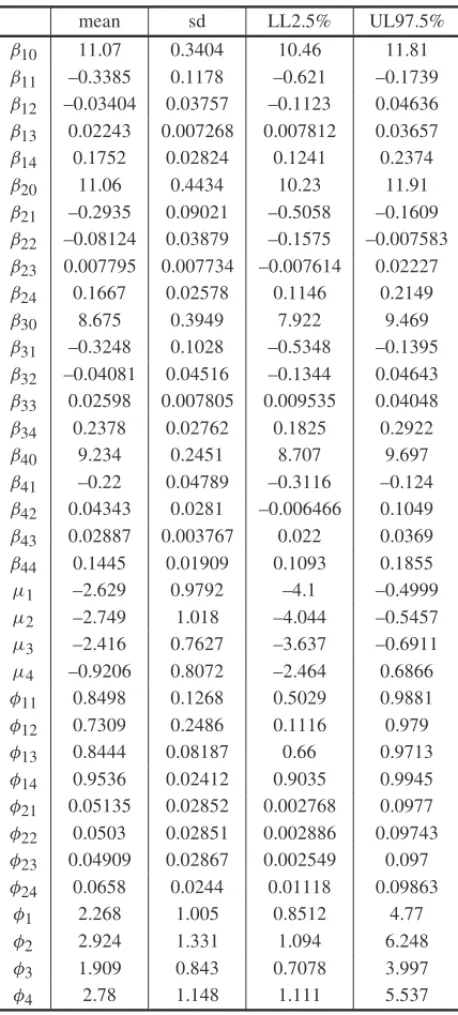
β10 11.07 0.3404 10.46 11.81
β11 –0.3385 0.1178 –0.621 –0.1739
β12 –0.03404 0.03757 –0.1123 0.04636
β13 0.02243 0.007268 0.007812 0.03657
β14 0.1752 0.02824 0.1241 0.2374
β20 11.06 0.4434 10.23 11.91
β21 –0.2935 0.09021 –0.5058 –0.1609
β22 –0.08124 0.03879 –0.1575 –0.007583 β23 0.007795 0.007734 –0.007614 0.02227
β24 0.1667 0.02578 0.1146 0.2149
β30 8.675 0.3949 7.922 9.469
β31 –0.3248 0.1028 –0.5348 –0.1395
β32 –0.04081 0.04516 –0.1344 0.04643
β33 0.02598 0.007805 0.009535 0.04048
β34 0.2378 0.02762 0.1825 0.2922
β40 9.234 0.2451 8.707 9.697
β41 –0.22 0.04789 –0.3116 –0.124
β42 0.04343 0.0281 –0.006466 0.1049
β43 0.02887 0.003767 0.022 0.0369
β44 0.1445 0.01909 0.1093 0.1855
µ1 –2.629 0.9792 –4.1 –0.4999
µ2 –2.749 1.018 –4.044 –0.5457
µ3 –2.416 0.7627 –3.637 –0.6911
µ4 –0.9206 0.8072 –2.464 0.6866
φ11 0.8498 0.1268 0.5029 0.9881
φ12 0.7309 0.2486 0.1116 0.979
φ13 0.8444 0.08187 0.66 0.9713
φ14 0.9536 0.02412 0.9035 0.9945
φ21 0.05135 0.02852 0.002768 0.0977
φ22 0.0503 0.02851 0.002886 0.09743
φ23 0.04909 0.02867 0.002549 0.097
φ24 0.0658 0.0244 0.01118 0.09863
φ1 2.268 1.005 0.8512 4.77
φ2 2.924 1.331 1.094 6.248
φ3 1.909 0.843 0.7078 3.997
φ4 2.78 1.148 1.111 5.537
(sd: standard deviation; LL2.5%: lower limit; UL97.5%: upper limit).
number of passengers to the Ribeir˜ao Preto airport with the increase of the dollar (1/Jan/2008 to 31/December/2014).
It is observed a positive value for the estimator of the regression parameter related to the months (0.02243) implying that there is a significant increase in the logarithm of the number of pas-sengers over the course of months. End of years lead to a significant increase in the number of passengers.
3.2.2 Passengers – S˜ao Jos´e do Rio Preto
Years, exchange rate and unemployment rate affect the number of passengers in the S˜ao Jos´e do Rio Preto airport (the 95% credibility interval does not contain zero), that is, the regression coefficients are statistically different from zero.
It is observed a positive value for the estimator of the regression parameter related to year (0.1667) which implies that there is a significant increase in the logarithm of the number of passengers to the S˜ao Jos´e do Rio Preto airport over the years (2008-2014).
It is observed a negative value for the estimator of the regression parameter related to the ex-change rate(−0.2935)which implies that there is a significant decrease in the logarithm of the number of passengers to the S˜ao Jos´e do Rio Preto airport with increase in the dollar (1/Jan/2008 to 31/December/2014).
It is observed a negative value for the estimator of the regression parameter related to the un-employment rate(−0.08124)which implies that there is a significant decrease in the logarithm of the number of passengers to the S˜ao Jos´e do Rio Preto airport with rising unemployment (1/Jan/2008 to 31/December/2014).
3.2.3 Passengers – Bauru/Arealva
Years, months and exchange rate are affecting the number of passengers in the Bauru airport (the 95% credible intervals do not contain zero), that is, the regression coefficients are statistically different from zero.
It is observed a positive value for the estimator of the regression parameter related to year (0.2378) which implies that there is a significant increase in the logarithm of the number of passengers in the Bauru airport over the years (2008-2014).
It is observed a negative value for the estimator of the regression parameter related to the ex-change rate(−0.3248)which implies that there is a significant decrease in the logarithm of the number of passengers in the Bauru airport with increase in the dollar rate (1/Jan/2008 to 31/De-cember/2014).
3.2.4 Passengers – Presidente Prudente
Years, months and exchange rate affect the number of passengers in the Presidente Prudente airport (the 95% credibility interval does not contain zero), that is, the regression coefficients are statistically different from zero.
It is observed a positive value for the estimator of the regression parameter related to year (0.1445) which implies that there is a significant increase in the logarithm of the number of passengers in the Presidente Prudente airport over the years (2008-2014).
It is observed a negative value for the estimator of the regression parameter related to the ex-change rate(−0.2200)which implies that there is a significant decrease in the logarithm of the number of passengers in the Presidente Prudente airport with increase in the value of dollar rate (1/Jan/2008 to 31/December/2014).
It is observed a positive value for the estimator of the regression parameter related to the months (0.1445) implying that there is a significant increase in the logarithm of the number of passengers with respect to months in the Presidente Prudente airport (end of year lead to increased number of passengers).
3.3 Bayesian analysis for the response log (cargo)
Considering, the cargo volume in the four airports, it is assumed the same prior distributions assumed for the passenger case, that is, Beta(1,1)prior distributions forφ1j, uniformU(0,0.1)
prior distributions forφ2j, Gamma(1.1)prior distributions forσ2jζ, normalN(0,1)prior
distri-butions forµj, normal N(10.1)prior distributions forβj o and N(0,1)prior distributions for
βjl, j =1,2,3,4;l =1,2,3,4. Also using the OpenBugs software, it is considered a burn-in
sample of size 21000; after that, we generated another 90,000 samples taking samples from 10 to 10 totaling a final sample size of 9,000 to get the posterior summaries of interest (see Table 2).
From the analyses of the results in Table 2, some important observations are reported in the following subsections.
3.3.1 Cargo – Ribeir˜ao Preto
Years, months and exchange rate affect the transportation of cargo in the Ribeir˜ao Preto air-port (the 95% credibility interval does not contain zero), that is, the regression coefficients are statistically different from zero.
It is observed a negative value for the estimator of the regression parameter related to the dollar exchange rate(−0.1753)which implies that there is a significant decrease in the logarithm of the freight transportation in the Ribeir˜ao Preto airport with the rise of the dollar rate.
Table 2– Posterior summaries – cargo.
mean sd LL2.5% UL97.5%
β10 10.76 0.5436 9.8 11.81
β11 –0.1753 0.06556 –0.3101 –0.04929
β12 –0.01155 0.05656 –0.1158 0.09262
β13 0.03134 0.01098 0.008729 0.05112
β14 0.09188 0.03801 0.01714 0.1584
β20 11.54 0.3735 10.83 12.33
β21 –0.378 0.1028 –0.5565 –0.1454
β22 0.02489 0.04428 –0.0643 0.1138
β23 –0.001191 0.008008 –0.01742 0.01418
β24 –0.06743 0.03149 –0.1328 –0.005542
β30 11.86 0.3814 11.06 12.58
β31 –0.3563 0.09295 –0.5425 –0.1762
β32 –0.08597 0.04153 –0.1671 9,80E–01
β33 0.02059 0.006896 0.0064 0.03353
β34 0.155 0.02563 0.106 0.2081
β40 8.312 0.6196 7.038 9.519
β41 –0.5819 0.1427 –0.8501 –0.2911
β42 0.1567 0.06345 0.03276 0.2824
β43 0.0363 0.0102 0.01685 0.05694
β44 0.1883 0.04512 0.1027 0.2724
µ1 –1.871 1.084 –3.403 0.4202
µ2 –3.147 0.6257 –3.828 –1.247
µ3 –2.339 0.8223 –3.67 –0.4718
µ4 –0.6796 0.8618 –2.327 1.011
φ11 0.7816 0.1544 0.4134 0.9768
φ12 0.5057 0.2594 0.0409 0.9401
φ13 0.847 0.08634 0.6412 0.9786
φ14 0.8933 0.05804 0.7487 0.9788
φ21 0.04734 0.0285 0.002384 0.09696
φ22 0.05025 0.02852 0.002646 0.09717
φ23 0.05043 0.02857 0.002579 0.09753
φ24 0.06185 0.02479 0.009566 0.0983
ζ1 1.141 0.5293 0.4524 2.451
ζ2 2.306 1.117 0.8192 5.143
ζ3 1.801 0.7774 0.7008 3.687
ζ4 2.811 1.261 1.054 5.9
(sd: standard deviation; LL2.5%: lower limit; UL97.5%: upper limit).
3.3.2 Cargo – S˜ao Jos´e do Rio Preto
Years and exchange rate affect the transportation of cargo in the S˜ao Jos´e do Rio Preto airport (the 95% credibility interval does not contain zero), that is, the regression coefficients are statistically different from zero. The other factors are not significative, possibly due to the presence of some outlier that could affect the obtained inference.
It is observed a negative value for the estimator of the regression parameter related to the dollar exchange rate(−0.3780)which implies that there is a significant decrease in the logarithm of the cargo transportation in the S˜ao Jos´e do Rio Preto airport with the rise of the dollar rate.
It is observed a negative value for the estimator of the regression parameter related to years
(−0.06743)which implies that there is a significant decrease in the logarithm of the transport of cargo in the S˜ao Jos´e do Rio Preto airport over the years.
3.3.3 Cargo – Bauru/Arealva
Years, months and exchange rate affect the transportation of cargo in the Bauru airport (the 95% credibility interval does not contain zero), that is, the regression coefficients are statistically different from zero.
It is observed a negative value for the estimator of the regression parameter related to the dollar exchange rate(−0.3563)which implies that there is a significant decrease in the logarithm of the cargo transportation in the Bauru airport with the rise of the dollar rate.
It is observed a positive value for the estimator of the regression parameter related to months (0.02059) implying that there is a significant increase in the logarithm of the amount of cargo transportation in the Bauru airport with respect to months (end of year lead to increased amount of cargo).
It is observed a positive value for the estimator of the regression parameter related to year (0.1550) which implies that there is a significant increase in the logarithm of the cargo in the Bauru airport over the years.
3.3.4 Cargo – Presidente Prudente
Years, months, unemployment rate and exchange rate affect the transportation of cargo in the Presidente Prudente airport (the 95% credibility interval does not contain zero), that is, the re-gression coefficients are statistically different from zero.
It is observed a negative value for the estimator of the regression parameter related to the dollar exchange rate(−0.5819)which implies that there is a significant decrease in the logarithm of the cargo transportation in the Presidente Prudente airport with the rise of the dollar rate.
It is observed a positive value for the estimator of the regression parameter related to year (0.1883) which implies that there is a significant increase in the logarithm of the cargo trans-portation in the Presidente Prudente airport over the years.
It is observed a positive value for the estimator of the regression parameter related to the unem-ployment rate (0.1567) which implies that there is a significant increase in the logarithm of the cargo transportation in the Presidente Prudente airport with rising unemployment rate.
3.4 Model fit and the estimated volatilities
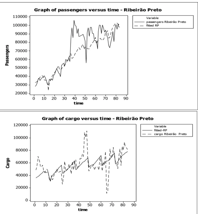
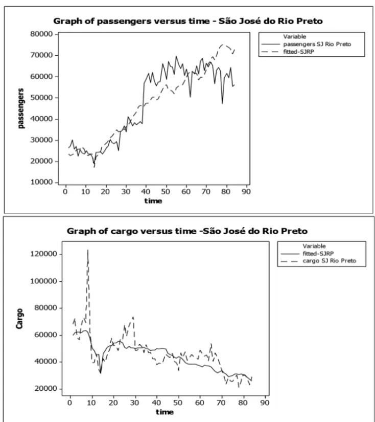
From the fitted model (1) for the data set related to the four airports (Ribeir˜ao Preto, S˜ao Jos´e do Rio Preto, Bauru/Arealva and Presidente Prudente), it is presented in Figures 2, 3, 4 and 5 the fitted means and the observed values for the air transport of passengers and cargo in the period ranging from January 01, 2008 to December 31, 2014.
In Figure 6, it is presented the graphs of the square roots for the volatilities considering the data set of the four airports (monthly counting of passengers and cargo).
From the plots of Figures 5 and 6, we get some important interpretations:
Passengers:
• There is great volatility for the number of passengers in the Ribeir˜ao Preto airport between month 40 (April, 2011) and month 50 (February, 2012). Outside of this period, there is a small volatility.
• Similar behavior is observed for the number of passengers in the S˜ao Jos´e do Rio Preto airport; the volatility increases at the end of the observed period, that is, close to the end of 2014 (year that starts big economic problems in Brazil).
• The Bauru airport has a great volatility regarding the number of passengers close to the month 25 (January, 2010) and month 55 (end of 2012).
• The Presidente Prudente airport has similar behavior regarding the volatility of the number of passengers as observed for the Bauru airport.
Cargo:
• The Ribeir˜ao Preto airport has a seasonal behavior regarding the volatilities in the transport of cargo (in some periods of the year there is greater volatility) where a large volatility occurs close to the month 65 which corresponds to the 2013 year.
• Similar behavior is observed regarding the cargo transportation in the S˜ao Jos´e do Rio Preto airport.
Figure 2– Time series for observed values and fitted values – passengers and cargo Ribeir˜ao Preto.
• The volatility of the data shows the dependence of the effective use of air modal struc-ture on the variability of passenger demand (tourism and corporate business) and cargo (potential of local production that requires the use of modal for the flow of products), directing efforts to the economic and financial viability of the national air transportation with emphasis on the best practices inherent in the concept of a hub.
4 CONCLUDING REMARKS
air-Figure 3– Time series for observed values and fitted values – passengers and cargo S˜ao Jos´e do Rio Preto.
ports in S˜ao Paulo State in the period of study. It was also possible, the identification of important factors affecting the amount of passengers and cargo for these airports.
Other important result: the fitted models used in this study can be of great importance in the prediction of number of passengers and amount of cargo, related to the economic factors consid-ered. These results are of great interest to airport managers as planning to build new large hubs for passengers or cargo as alternative for the great airports located in S˜ao Paulo or Campinas cities.
Figure 4– Time series for observed values and fitted values – passengers and cargo Bauru/Arealva.
In addition, it is important to point out that the use of a Bayesian approach with MCMC (Markov Chain Monte Carlo) methods is facilitated using available free software like OpenBugs, which gives a great simplification in the computational work to get the posterior summaries of interest.
Figure 5– Time series for observed values and fitted values – passengers and cargo Presidente Prudente.
For a future work, it would be possible to consider other volatilities structures and to compare the obtained results with results originating from other statistical approaches, as for example, using generalized linear models for the counting data in the original scale and not in the logarithm scale as considered in this study.
Figure 6– Square roots for volatilities (passengers/cargo) for the airports.
ACKNOWLEDGMENTS
The authors are very grateful to the Editor and referees for their helpful and useful comments that improved the manuscript.
REFERENCES
[1] ALUMUR SA & YAMAN HK. 2012. Hierarchical multimodal hub location problem with time-definite deliveries.Transportation Research,48: 1107–1120.
[3] BARTODZIEFP, DERIGSU, MALCHEREKD & VOGELU. 2009. Models and algorithms for solving combined vehicle and crew scheduling problems with rest constraints: an application to road feeder service planning in air cargo transportation.OR Spectrum,31(2): 405–429.
[4] BOLLERSLEVT. 1986. Generalized autoregressive conditional heteroscedasticity.Journal of Econo-metrics,31: 307–327.
[5] BOUGEROLP & PICARDN. 1992. Stationarity of GARCH processes and of some nonnegative time series.Journal of Econometrics,52: 115–127.
[6] BOWENJTJ. 2012. A spatial of Fedex and UPS: hubs, spokes, and network structure.Journal of Transport Geography,24: 419–431.
[7] DANIELSSONJ. 1994. Stochastic volatility in asset prices: estimation with simulated maximum like-lihood.Journal of Econometrics,61: 375–400.
[8] ENGLERF. 1982. Autoregressive Conditional Heteroscedasticity with Estimates of the Variance of United Kingdom Inflation.Econometrica,50(4): 987–1007.
[9] FENGB, LIY & SHENZJ. 2015. Air cargo operations: Literature review and comparison with pratices.Transportation Research, Part C,56: 263–280.
[10] GARDINERJ, HUMPREYI & ISONS. 2005. Freighter operators’ choice of airport: A three-stage process.Transport Reviews,25(1): 85–102.
[11] GARDINERJ & ISON S. 2008. The geography of non-integrated cargo airlines: An international study.Journal of Transport Geography,16(1): 55–62.
[12] GARDINERJ, HUMPREYI & ISONS. 2005. Factors infuencing cargo airlines’ choice of airport: An international survey.Journal of Air Transport Management,11(6): 393–399.
[13] GELFANDAE & SMITHAFM. 1990. Sampling-based approaches to calculating marginal densities. Journal of the American Statistical Association,85(410): 398–409.
[14] GHYSELSE. 1996. Stochastic volatility. In: Statistical methods on finance, North-Holland.
[15] GROSSOMG & SHEPHERDB. 2011. Air cargo transport in APEC: Regulation and effects on mer-chandise trade.Journal of Asian Economics,22: 203–212.
[16] HEINICKEK. 2016. World Air Cargo Forecast. 2006/2007.
[17] HUANGK & LUH. 2015. A linear programming-based method for the network revenue management problem of air cargo.Transportation Research Procedia,7: 459–473.
[18] KARABY & TANSELB. 2001. The latest arrival hub location problem.Manage Sciences,47: 1408– 1420.
[19] KIMS & SHEPHARDN. 1998. Stochastic volatility: likelihood inference and comparison with arch models.Review of Economic Studies,65: 361–393.
[20] LAKEWPA, TOKY & CHERNA. 2015. Determinants of air cargo traffic California.Transportation Research, Part A,80: 134–150.
[21] LEUNG LC, VAN HUI Y, WANGY & CHENG. 2009. A 0-1 LP model for the integration and consolidation of air cargo shipments.Operational Research,57(2): 402–412.
[23] LINCC, LINYJ & LINDY. 2003. The economic effects of center-to-center directs on hub-and-spoke networks air express common carriers.Journal of Air Transport Management,9: 255–265.
[24] MEYERR & YUT. 2000. Bugs for a Bayesian analysis of stochastic volatility models.Econometrics Journal,3: 198–215.
[25] MORRELPS & PILONRV. 1999. KLM and Northwest: a survey of the impact of a passenger aliance on cargo servisse characteristics.Journal of Air Transport Management,5: 153–160.
[26] NELDERJA & WEDDERBURNRWM. 1972. Generalized linear models.Journal of the Royal Statis-tical Society, Series A,135(3): 370–384.
[27] NELSONDB. 1990. Stationarity and persistence in the GARCH(1,1)model.Economy Theory,6: 318–334.
[28] OKTALH & OZGERA. 2013. Hub location air cargo transportation: A case study.Journal of Air Transport Management,27: 1–4.
[29] ONGHENAE. 2011. Integrators in a changing world. Critical issues in air transport economics and business. London: Routledge, 112–132.
[30] PETERSENJ. 2007. Air freight industry – white paper. Research Report, Georgia Institute of Tech-nology.<www.scl.gatech.edu/industry/industry-studies/AirFreight.pdf> Access 06 jan. 2016.
[31] SCHOLZAB & COSSELJ. 2011. Assessing the importance of hub airports for cargo carriers and its implications for a sustainable airport management.Research in Transportation Business & Manage-ment,1: 62–70.
[32] SMILOWITZKR & DAGANZOCF. 2007. Continuum approximation techniques for the design of integrated package distribution systems.Networks,50: 183–196.
[33] SMITH AFM & ROBERTS GO. 1993. Bayesian computation via the Gibbs sampler and related Markov chain Monte Carlo methods.Journal of the Royal Statistical Society, Series B, Methodologi-cal,55(1): 3–23.
[34] SPIEGELHALTERDJ, THOMASA, BESTNG & LUNDD. 2003. Winbugs user manual. Cambridge. United Kingdon: MRC Biostatistics Unit.
[35] TANPZ & KARABY. 2007. A hub-covering model for cargo delivery systems.Networks,49: 28–39.
[36] YUJ. 2002. Forecasting volatility in the New Zeland stock market.Applied Financial Economics, 12: 193–202.
[37] WUCJH & HAYASHIY. 2011. Airport Attractiveness Analysis through a Gravity Model: A Case Study of Chubu International Airport in Japan,Proceedings of the Eastern Asia Society for Trans-portation Studies, Vol. 8.