Abstract
We explore, in this paper, the demands and behavior on fasteners supplying sheathing-based bracing of gravity loaded cold-formed studs and wall assemblies. The studies are carried out by shell finite element (FE) models, which are compared to analytical solutions and previously completed laboratory tests conducted by the authors. The connection between the sheathing and the stud should be able to develop enough resistance to restrain global buckling of the studs; therefore, special attention has to be given to the demands on these connections for design. Local buckling and stress concentrations may damage some connections and re-distribution of forces should be ensured. Classical practice for determining fastener demand – i.e., the 2% rule – may be defi-cient. An analytical method developed for determining fastener demand is compared to the FE models presented in this paper; the analytical method results in a reasonable prediction of the fastener forces in wall studs.
Keywords
fastener, cold-formed steel, stud wall
Fastener Demands for Sheathing-Braced
Cold-Formed Steel Stud Gravity Walls
1 INTRODUCTION
Cold-formed steel may be used to frame the walls, floors, and roofs of modern buildings. The indi-vidual cold-formed steel members (studs) have sheathing attached to provide appropriate architec-tural enclosures. This sheathing also serves to brace the cold-formed steel studs under load. Cur-rent design methods are highly developed regarding the design of isolated cold-formed steel mem-bers such as columns and beams, but cold-formed steel wall studs that rely on sheathing for bracing are not fully addressed.
Significant work has been conducted on sheathing-braced cold-formed steel stud walls, Okasha (2004), Fiorino et al. (2007), and Chen et al. (2006) have concentrated their efforts in determining the resistance of the stud-to-sheathing connection; while Miller and Pekoz (1993), Winter (1960), and Simaan and Pekoz (1976) have explained their implications on the wall stud resistance, but few
Luiz Carlos M. Vieira Junior a Benjamin W. Schafer b
a University of Campinas,
email: [email protected] b Johns Hopkins University,
email: [email protected]
http://dx.doi.org/10.1590/1679-78252428
have specifically investigated fastener demands. The commentary of AISI-S211 (2007), based on the research conducted by Winter (1960), states that a fastener-sheathing assembly shall be designed for a load equal to 2% of the axial load, also know as “2% rule”.
It is involved to determine fastener demand experimentally; not only is it difficult to instrument fasteners and sheathing, but also each connection would have to be instrumented individually. For the reasons mentioned above, a shell FE model was developed. In the FE models we can easily ana-lyze each demand on the fastener – lateral, axial, and rotational – separately, which facilitates the understanding of the forces developed in the connections as they attempt to brace the stud under applied gravity load.
2 FE MODELS
2.1 Single-Column FE Model
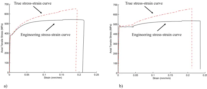
Fastener demands are explored by means of shell FE models developed to be similar to previously conducted sheathed single-column tests and sheathed wall-stud assemblies, Simaan and Pekoz (1976) and Vieira et al. (2011) and . As in the tests, all the models simulate 362S162-68 studs and 362T125-68 tracks, AISI S200 (2007). The single-column model and full wall-stud models share many modeling characteristics, such as: element type, stress-strain curve for the material, boundary conditions and initial imperfections, but they are different in terms of geometry. The single columns are 2.44m (8ft) long connected on both ends to a 0.61m (2ft) track, the sheathing is also 2.44m (8ft) long but is only 0.46m (18in) wide and it is connected to the stud every 0.30m (12in), while it is connected at every 0.15m (6in) to the track. We modeled a 2.44x2.44m (8x8ft) (two sheathing 1.22x2.44m (4x8ft) on each side) wall-stud, with 5 studs connected to the track on their ends, studs are connected to the sheathing at every 0.30m (12in) on the field and every 0.15m (6in) on the edg-es of the sheathing. In the tedg-ests, the studs are loaded through a loading plate 0.3m (12in) long and 0.10m (3.6in) wide to insure that only the stud is engaged in direct bearing and never the The models are built in ABAQUS (2007), using S4R1 shell elements to model stud, track and sheathing. The material steel is simulated using the stress-strain curves depicted in Figure 1, which are transformed from engineering stress to true stress2 for use in ABAQUS (2007). The material model chosen to represent the steel is non-linear, and it considers metal plasticity (von Mises yield surface) and isotropic hardening. The sheathing is modeled as an orthotropic material with Young’s modulus (E) and shear modulus (G) as discussed in Vieira (2011) (OSB – E=6,426 MPa (932 ksi), shear G=1,310 MPa (190 ksi), thickness=7/16in; Gypsum – E=993 MPa (144 ksi), G=552 MPa (80 ksi)), thickness=1/2in and =0.3. The modified Riks method is used to solve the nonlinear model.
1 S4R elements are used rather than S4R5, because S4R elements allow the rotation on plane of the element to be
restricted.
2 Engineering strain (
0) is transformed to true strain () by the relationship =ln(1+0), thus by assuming a
Latin American Journal of Solids and Structures 13 (2016) 1167-1185 Figure 1: Stress-strain curve used for simulating: a) stud and b) track.
The stud-to-track fasteners are idealized by coupling all the degrees of freedom except the rota-tion around the axis of the fastener and the stud-to-track contact is idealized by coupling all the displacements except the displacement on the plane of the track’s web (stud end is free to slide). A displacement is applied to a master node that transfers this displacement to a rigid body that repre-sents the isolation plate on the track web used to load the stud.
The models have their geometry altered by an initial imperfection, which is considered as either a small initial imperfection (25th percentile) or a large initial imperfection (75th percentile). The magnitude of the initial imperfection is depicted in Table 1 and it follows Schafer and Pekoz (1998) regarding local imperfections (“d1” and “d2”) and Schafer and Zeinoddini (2008) regarding global imperfections (bow, camber and twist).
Reference Type of
imperfection
P(Δ < d)* 25th
%ile
75th %ile
Schafer and Peköz (1998) Local (d1/t) Distortional (d2/t)
0.14 0.64
0.66 1.55
Schafer and Zeiniddini (2008)
Bow Camber
Twist
L/4755 L/6295 0.46º
L/1659 L/2887 1.23º
* “Probability that a randomly selected imperfection value, Δ, is less than a discrete deterministic imperfection, d.” Schafer and Pekoz (1998).
Table 1: Imperfection applied on studs.
for example and for spring orientation. For models in this case the diaphragm stiffness (kxd), the
rotational stiffness provided by the sheathing (kϕ), and the out-of-plane stiffness (ky) are
However, if the sheathing is being included directly in the model, the same three variables are not considered since the sheathing is in place and it will automatically take in account these stiffnesses. The stiffness provided by the sheathing in the axial direction may also be considered and since is no specific value for kz and kϕx, we have used the same values of kx and k respectively, which in
fact is a lower-bound value for these stiffnesses, Table 2.
Sheathing
Material Spring
Sheathing in place, springs idealize just
the fastener
No sheathing, springs idealize fastener
and sheathing
OSB
Kx=Kz (N/mm)
Ky (N/mm)
Kϕ=Kϕx (N.mm/rad)
1241 N/A 136660 971 0.374 95309 Gypsum
Kx=Kz (N/mm)
Ky (N/mm)
Kϕ=Kϕx (N.mm/rad)
426 N/A 129745 427 0.087 95987
Table 2: Spring stiffness used in the FE models (fastener spacing considered is 305mm (12in)), Figure 2 depicts the spring orientation. See Vieira and Schafer (2013). For more information about how to
determine the springs’ stiffnesses.
x
y
z
k
xk
yk
zx
y
z
k
xk
yk
z=k
a) b)
Latin American Journal of Solids and Structures 13 (2016) 1167-1185
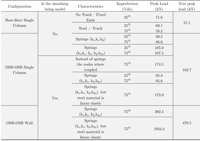
A series of shell FE collapse models (i.e. geometric and material nonlinear models with imper-fections) for the sheathed single-column tests with varying degree of sophistication are summarized in Table 3. The first set of FE models presented compares the end boundary conditions in the mod-els to the Bare-Bare (denotes that no sheathing was present on either flange face of the test) single-column test, 2.44m (8feet) long, Table 3. The model that simulates stud and track when compared to a column with fixed-fixed ends did not show a great difference, and both models represent a slighter higher peak than found in the test reported in Vieira and Schafer (2013). Our idealization of a boundary condition that directly couples nodes instead of using contact elements leads to a slighter stiffer system, but the presence of the track is important to establish the connection be-tween sheathing and track, which, as it will be shown further, develops an important role in dis-tributing the load to the stud and at the same time bracing it.
The second set of models concentrates on understanding the springs that should be considered in order to simulate the tests (this all without considering the sheathing explicitly, bot now consid-ering tests with sheathing-bracing). In these models we found that if we only consider the springs kx, ky and kϕ, the models lead to a peak load around 16% lower than the peak load in the test,
Table 3. However if we add kz and kϕx, which are responsible for the contribution of the sheathing
in the longitudinal direction of the stud, the results are in excellent agreement with the test. Sug-gesting modest composite action is present even though the vertical load is isolated.
The third set of models also compares the same single-column test (OSB-OSB, 2.44m (8feet)) to the tests, but this time the sheathing is explicitly modeled (instead of smeared into a spring stiff-ness); thus the spring stiffness is changed as discussed above and provided in Table 2. In the first model, instead of using springs, we coupled the displacements at the stud and track to the sheath-ing, which created an upper bound value for the peak loads (70% higher that the test). When we actually modeled the stud and track connected to sheathing through spring elements we found a peak load only 7% lower than found in the tests, which we consider a good prediction. Also simu-lated (an addendum to the third set of models) was analysis considering a linear elastic steel mate-rial: our goal with this model is to understand the fastener forces in the model if there is no plastic deformation in place. In the case of the single-column models the difference in the fastener forces are small, but the same is not observed in the wall-stud model, because in the latter model plastici-ty of the stud-to-track connection plays an important role.
Configuration Is the sheathing
being model Characteristics
Imperfection (%ile) Peak Load (kN) Test peak load (kN) Bare-Bare Single Column No
No Track / Fixed
Ends 25
th 71.6
57.1
Stud + Track 25
th 75th 69.1 58.2 OSB-OSB Single Column
Springs (kx,ky,kϕ) 25
th 75th 89.5 86.6 102.7 Springs
(kx,ky, kz, kϕ,kϕx)
25th 75th
105.0 107.5
Yes
Instead of springs the nodes where
coupled
75th 174.5
Springs (kx,kz, kϕ,kϕx)
25th 75th
95.8 95.6 Springs
(kx,kz, kϕ,kϕx), but
steel material is linear elastic
75th 173.9
OSB-OSB Wall
Springs
(kx,kz, kϕ,kϕx) 75
th 392.4
479.5 Springs
(kx,kz, kϕ,kϕx), but
steel material is linear elastic
75th 1934.4
Table 3: FE models results.
A closer look into the models leads to several conclusions regarding the fastener forces (i.e. the forces at the fastener locations that supply bracing to the stud). The first model to be analyzed in depth is considered the simplest model of this series, which considers only the springs kx, ky and kϕ,
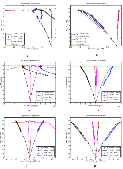
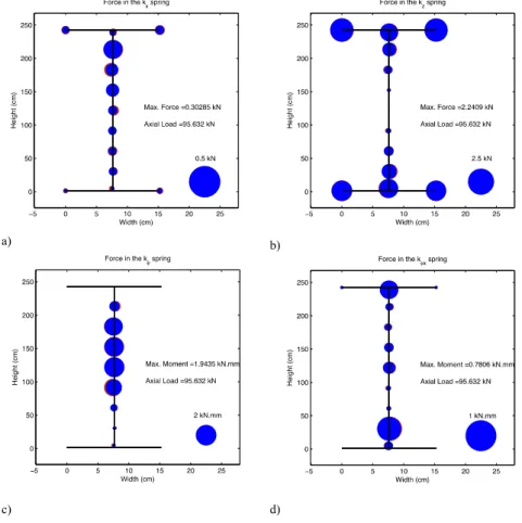
and the board is not explicitly modeled, Figure 3. Figure 4 depicts the force and moments in the springs for different initial imperfections, different sides where the sheathing is connected (side 1 and 2), and different positions: ends (first spring on the stud, 50.8mm (2in) from the end), and cen-ter of stud. Local and distortional buckling are modestly affected by the presence of springs, but the springs play an important role in restricting global buckling, that includes: weak axis buckling and flexural-torsional buckling. This simple model shows that at peak load the forces on the kx springs
are at its maximum magnitude at the center of the stud, but after peak load due to local buckling, the maximum force in the springs are transferred from the center to the ends, where local buckling happens: Figure 3 (b, c). It is also shown in Figure 4 that for a 75th percentile magnitude of initial imperfection the fastener force is higher than a 25th percentile of initial imperfection (as expected); therefore, further studies are based on models that have its geometry altered by a 75th percentile initial imperfection – i.e., a plausible worst case scenario. Another conclusion is that the force at the ky springs are very small, this is explained by the nature of the problem, since strong-axis buckling
Latin American Journal of Solids and Structures 13 (2016) 1167-1185
in the rotational spring is also very small compared to the capacity of the connection, in the tests reported in Vieira and Schafer (2013). the maximum moment at the k spring for OSB is on the
average 47.45kN.mm (420lbf.in (351lbf.in/in*12in)) while in the models the maximum moment at the spring is of 3kN.mm (26.55 lbf.in).
x
z
y
a) b)
c)
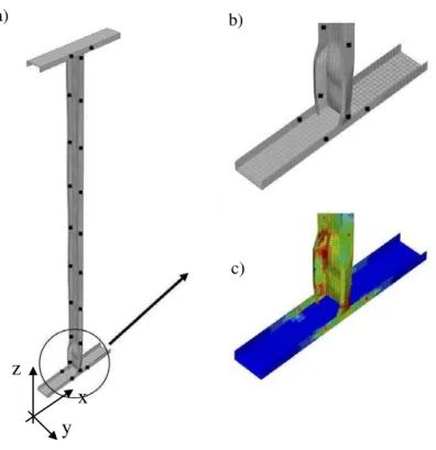
Figure 3: Simple model that considers only kx, ky, kϕ, and sheathing is simulated by means of springs
a) Single-column model, springs are depicted in black dots, b) Zoomed view of stud end where local buckling takes place, c) von-Mises stresses on stud end.
Another single-column model interesting to explore is the one that considers kx, kz, kϕ, kϕx, and
the sheathing, Figure 5. Figure 6 depicts the force and moment in the springs at peak load for the model of Figure 5. The demands on side 1 and 2 are plotted in different colors, but since the single-column model presents a symmetric behavior regarding the sides, the plots of side 1 and 2 are al-ways superimposed and little difference can be seen. In the tests reported Vieira and Schafer (2013). , the average peak load carried in the translation test is 2.58kN (0.58 kips), therefore the demand in the translational springs should not exceed the peak load reported in the tests, as it is observed in Figure 6 (a, b) in the value of the maximum force. The kx spring has the greatest magnitude close
to the ends where the stud buckles in a local mode, Figure 5 (c, d). While the kz spring has more
kϕ spring has greatest demands in the middle of the stud. This shows that the kϕ spring is provid-ing a small contribution to restrain flexural-torsional bucklprovid-ing. Nonetheless, the kϕx springs have
their greatest demands at the ends, showing that the kϕx springs help restrain the stud in
strong-axis buckling. The primary conclusion with this model is that the group of springs and the sheath-ing are able to restraint global bucklsheath-ing and hence the stud buckles in local bucklsheath-ing.
Figure 4: Simple model that considers only kx, ky, kϕ, and sheathing is simulated by means of springs
Latin American Journal of Solids and Structures 13 (2016) 1167-1185
x z
y
a) b) c)
d)
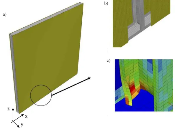
Figure 5: Model that considers kx, kz, kϕ, kϕx, and sheathing is also simulated a) Overall view of FE model, steel
members are represented in gray and OSB in brown, b) Part of the sheathing is removed to show the stud, d) Zoomed view of stud end where local buckling takes place, c) von Mises stress on stud end.
Figure 6: Force and Moment in the springs at peak load for model that considers kx, kz, kϕ, kϕx,
2.2 Full Wall Stud FE Model
2.2.1 Wall Stud Sheathed with OSB on Both Sides (OSB-OSB)
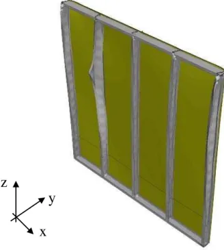
While the single-column models show perfect symmetry and a very predictable behavior, the full wall-stud model opens a new horizon to be explored; in fact, an asymmetric horizon replete with load re-distribution. It is worth recalling that the steel members on the edges (studs and tracks) are connect-ed to sheathing every 152mm (6in.), the field studs are connectconnect-ed to sheathing every 254mm (12in.), and the stud in the middle that is connected to two sheathing boards is connected by two lines of fasteners (one line each board), every 152mm (6in.). The full wall shell FE model is depicted in Figure 7.
x
z
y
a)b)
c)
Figure 7: FE Model considers kx, kz, kϕ, kϕx, and sheathing is also simulated (OSB-OSB) a) Overall view of
FE model, steel members are represented in gray and OSB in brown, b) Zoomed view of stud end where local buckling takes place, the sheathing is partially removed to provide view of the stud, c) von Mises stress on stud end, special attention is brought to the stud-to-track connection where plastic failure takes place.
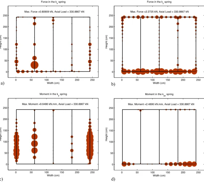
The kx spring has highest demands at the ends, where the stud is undergoing local buckling. At
the peak load, the corners are the places that the springs present the highest demands, Figure 8(a). The kx spring is explored in more detail in the following. The kz spring reaches its full capacity
Latin American Journal of Solids and Structures 13 (2016) 1167-1185
load levels compared to their resistance, but are still important for understanding the whole behav-ior of the system, Figure 8(c, d). The higher loads in the kϕx spring are at the end of the studs and
track, implying that kϕx helps restrain flexural-torsional buckling of the stud and bending of the
track flanges. But kϕ loads are higher at the edge studs; due to the asymmetric contribution of the sheathing to the stud. At the edges, the flange of the stud is responsible for anchoring the sheathing that is bending out of its plane, while at the other studs the bending moment is counterbalanced by the continuation of the sheathing.
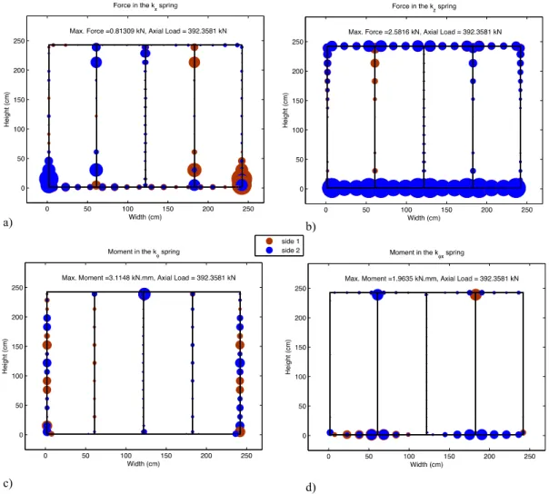
Figure 8: Force and Moment in the springs at peak load for non-linear sheathed wall-stud model (kx, kz, kϕ, kϕ) (OSB-OSB). The biggest marker is equivalent to the maximum moment or force of each picture.
Special attention is warranted for the kx spring (Figure 9), which is the spring (bracing
defines the side that has greatest demands. For example, the second stud from left to right has a sheathing contribution from the right side of the stud higher than from the left side and thus the spring on side 2 receives more load than side 1, and the problem is inverted on the fourth stud and thus the spring that receives more load is on side 1. However, if both plots are superposed as in Figure 8(a) the overall load plot is symmetric. Another interesting observation is the force distribu-tion in kx over different load steps. Until about 85% of the peak load, Figure 9(a, b), the studs that
has higher loads in the springs are the field studs (second and fourth studs), and this is due to the development of local buckling at the end of those studs, Figure 7(b), but after 85% of peak load the force on the field studs does not increase and the connections in the corners start taking more lat-eral load. There is always some doubt about what is the least favorable situation: higher fastener spacing (field studs) or less sheathing contribution (edge studs). This study shows that the sheath-ing may be able to redistribute the loads and balance either the lower number of fasteners or the smaller effective width of the sheathing, but the redistribution depends on the extent to which local buckling is developed at the ends of the field studs.
Figure 9: Distribution of the forces in the kx springs varying side that is being attached and axial load
Latin American Journal of Solids and Structures 13 (2016) 1167-1185
2.2.2 Wall Stud Sheathed with OSB on One Side Only (OSB-BARE)
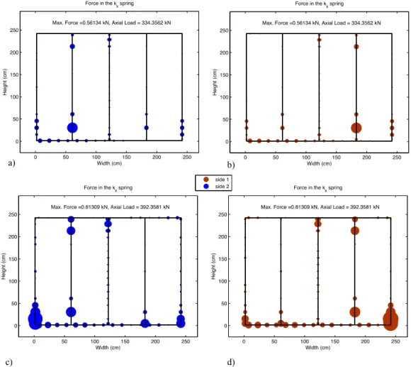
Another interesting case to be explored is a wall stud sheathed with OSB on one side only (OSB-BARE), Figure 10. There is some concern that since the studs failed in flexural-torsional buckling during the tests the fastener demand on walls with studs sheathed on one side only would be bigger than walls sheathed on both sides. The models actually show that the fasteners demands in OSB-BARE walls are lower than in OSB-OSB walls, see Figure 10 and Figure 11, which correspond well to what was seen in the tests. In the OSB-BARE tests the connections were not fully damaged after peak load; however in OSB-OSB tests the connections were fully damaged, especially close to the ends where local buckling takes place. Although the OSB-BARE condition is not a beneficial one in terms of strength, it is not observed to be problematic in terms of bracing demands developed in the stud to sheathing fasteners.
x
z
y
Figure 10: FE Model considers kx, kz, kϕ, kϕx, and OSB sheathing on one side only.
The kx springs have the greatest demands at the stud that buckles first – second stud (left to
right). Unlike in the OSB-OSB model, the force doesn’t redistribute to the edge studs, although the kx springs at the edge studs still play an important role in bracing the wall, as can be observed by
the amount of force in the kx springs at the edge studs, see Figure 11(a). The kz springs follow the
by the sheathing asymmetry, Figure 11(d), but the moment resisted by the spring looses its sym-metry as depicted in Figure 8(d).
Figure 11: Force and Moment in the springs at peak load for non-linear sheathed wall-stud model (kx, kz, kϕ, kϕ)
(OSB-BARE). The biggest marker is equivalent to the maximum moment or force of each picture.
2.3 Necessary Strength of Connections
The 2% bracing rule has been used to imply that if the fasteners are designed such that the sum of the forces on the fasteners is at least 2% of the axial load they should provide adequate bracing. This empirical rule has been used implicitly or explicitly since 1962 by the cold-formed steel design codes3. In 2008 Schafer et al. (2008) showed that following the assumptions established by Winter
Latin American Journal of Solids and Structures 13 (2016) 1167-1185
(1960) the actual necessary bracing force is in fact 1% of the axial load, therefore the design codes in essence adopted a safety factor of 2. The 2% rule can be compared against the FE models. Figure 12 depicts the axial load versus the sum of the fastener forces on the second stud from left to right on the sheathed wall-stud model (see Figure 8(a) for distribution across the fasteners). The curve represents a typical magnitude of load carried by the springs, which exceeds 2% of the axial load at peak load. In fact, the comparison between the 2% rule and the FE model are important just to give an idea of fastener demand, since in the FE model the fastener force are magnified where the stud undergoes local buckling (again see Figure 8(a)) and the 2% rule conceptually only takes in account the strength necessary to restrain global buckling in a pinned-pinned column.
0.5 1 1.5 2 2.5 3 3.5 4 4.5 0
10 20 30 40 50 60 70 80
Sum of fasteners force on stud 2 (% of axial load)
Axial Load (
k
N)
Figure 12: Sum of fasteners force in the kx spring on second stud (left to right) of sheathed wall-stud
(Figure 8(a)) versus axial load.
3 COMPARISON BETWEEN FE MODELS AND ANALYTICAL SOLUTION
For global buckling, the fastener demands can be analytically approximated based on an energy formulation employing beam theory, discrete springs at the bracing locations, and an assumed de-formation shape as a Fourier sine series as provided in Vieira and Schafer (2013). A geometric non-linear shell FE model of a 362S162-68 stud, simply supported, with kx, kz, kϕ springs 305 mm (12
in.) o.c. along the length, is used to verify the analytical solution. It is worth emphasizing that the analytical solution is for global buckling only, hence the fastener forces are only related to restrict-ing global bucklrestrict-ing. Purely for verification purposes, to eliminate local and distortional bucklrestrict-ing, the stud thickness is changed from 1.67 mm (0.0656 in.) to 6.35 mm (0.25 in.).
demand of the center fastener shows similar results, Figure 13(a). If camber imperfection or camber and twist imperfections are applied, the shell FE and the analytical solution may lead to a different prediction of the fastener force, Figure 13(b and c). A better approximation is given if the three buckling modes (minor-axis flexure and the two coupled flexural-torsional modes) of the analytical solution are taken in account to amplify the lateral displacement, Figure 13(d). It is common to consider only the first mode, because in classical flexural buckling the other modes represent only a small contribution to the displaced shape, but in buckling of singly-symmetric studs flexural-torsional, and weak-axis buckling are often at similar elastic buckling values and magnification in both modes as load (P) goes to the buckling load (Pcr). For best accuracy in the fastener force
pre-diction it is important to consider the additional buckling modes.
Figure 13: Fastener demand in the x direction. Comparison between FE model and analytical solution of a simple-supported stud of geometry similar to 362S162-68, but thickness of 6.35mm (0.25in.) a) Stud with only twist initial imperfection (twist=1.23o), b) Stud with twist and camber initial imperfection (twist=1.23o,
camber=L/2887), c) Stud with all global initial imperfections (twist=1.23o, camber=L/2887, bow=L/1659), d) Stud with all global initial imperfections (twist=1.23o, camber=L/2887, bow=L/1659), and analytical
Latin American Journal of Solids and Structures 13 (2016) 1167-1185
The analytical solution is also compared to the OSB single-column and the full-wall OSB-OSB shell FE model, as depicted in Figure 14. To take in account the clamped-clamped boundary conditions of the model, the analytical solution is found for a buckling length of one half of the ac-tual column height. Even though the shell FE models in this case consider not only global, but also local and distortional initial imperfection, the analytical solution still results is a reasonable predic-tion of the fastener forces for the wall studs. It is worth noting that the fasteners at mid-height are compared to the analytical solution since this is where first mode global is maximized, but these fasteners are little influenced by local buckling deformations in this case.
Figure 14: Comparison between FE model and analytical solution considering all the buckling modes in a wall stud as depicted in Figure 10.
4 STUD-TO-TRACK DEMAND
It was found in the shell FE models that the maximum shear force on the stud-to-track fasteners is approximately 5% of the axial load, but it is worth pointing out again that the FE models consider perfect contact between stud end and track web. More information on this topic may be found in Laboube and Findlay (2007).
5 CONCLUSIONS
developed at the ends of the field studs and is thus a function of the stud cross-sectional slender-ness. Wall stud assemblies with sheathing of very different stiffness; for example oriented strand board (OSB) on one side and bare on the other, may not provide significant restraint, but do not result in fastener demands that exceed wall studs with similar sheathing stiffness (e.g. OSB on both sides). A simple analytical model is shown to reasonably predict the fastener demands, but a better approximation is given if all three buckling modes of the analytical solution are taken in account when amplifying the lateral displacement. The load carried by the springs does exceed the 2% brac-ing rule necessary to restrain global bucklbrac-ing, but it is shown that the load is magnified where the stud undergoes local buckling.
Acknowledgments
The authors thank the American Iron and Steel Institute, the Steel Stud Manufacturers Association and São Paulo Research Foundation (FAPESP) for funding this research (grant #2014/26217-9). Any opinions, findings, and con-clusions or recommendations expressed in this material are those of the authors only and do not necessarily reflect the views of the sponsors.
References
ABAQUS, ABAQUS/Standard Version 6.7-1, D. Systemes, Editor 2007.
AISI-S200, North American Standard for Cold-Formed Steel Framing – General Provisions. American Iron and Steel Institute, 2007.
AISI-S211, North American Specification for the Design of Cold-Formed Steel Structural Members. American Iron and Steel Institute, 2007.
Chen, C.Y., A.F. Okasha, and C.A. Rogers, Analytical Predictions Of Strength and Deflection Of Light Gauge Steel Frame/Wood Panel Shear Walls. Advances in Engineering Structures, Mechanics & Construction, 2006: p. 381-391. Fiorino, L., G. Della Corte, and R. Landolfo, Experimental tests on typical screw connections for cold-formed steel housing. Engineering Structures, 2007. 29(8): p. 1761-1773.
Laboube, R.A. and P.F. Findlay, Wall stud-to-track gap: Experimental investigation. Journal of Architectural Engi-neering, 2007. 13(2): p. 105-110.
Miller, T.H. and T. Pekoz, Behavior of cold-formed wall stud-assemblies. Journal of structural engineering New York, N.Y., 1993. 119(2): p. 641-651.
Okasha, A.F., Okasha, A.F., Performance of Steel Frame/Wood Sheathing Screw Connections Subjected to Mono-tonic and Cyclic Loading, 2004, McGill University in Civil and Environmental Engineeering, McGill University: Montreal.
Schafer, B.W. and T. Peköz, Computational modeling of cold-formed steel: Characterizing geometric imperfections and residual stresses. Journal of Constructional Steel Research, 1998. 47(3): p. 193-210.
Schafer, B.W. and V.M. Zeinoddini. Impact of global flexural imperfections on the cold-formed steel column curve. in
19th International Specialty Conference on Recent Research and Developments in Cold-Formed Steel Design and Construction. 2008.
Schafer, B.W., O. Iourio, and L.C.M. Vieira Jr, Notes on AISI Design Methods for Sheathing Braced Design of Wall Studs in Compression, in A supplemental report for AISI-COFS Project on Sheathing Braced Design of Wall Studs,
2008, The Johns Hopkins University: Baltimore.
Latin American Journal of Solids and Structures 13 (2016) 1167-1185 SSMA, Product Technical Information - Complies with 2006 IBC. Steel Stud Manufacturers Association, 2010. Vieira, L., Jr. and Schafer, B. W. Behavior and Design of Sheathed Cold-Formed Steel Stud Walls under Compres-sion in J. Struct. Eng. 139, SPECIAL ISSUE: Cold-Formed Steel Structures, 772–786, 2013.
Vieira, L.C.M. ; Shifferaw, Yared ; Schafer, B.W. Experiments on sheathed cold-formed steel studs in compression in Journal of Constructional Steel Research, v. 67, p. 1554-1566, 2011.
Vieira, L.C.M.J., Behavior and Design of Sheathed Cold-Formed Steel Stud Walls under Compression, Johns Hop-kins University: Baltimore. p. 239, 2011.