Corresponding author: Shihua Zhang, Network Information Centre, Hunan Institute of Engineering, Xiangtan, Hunan, China, e-mail: [email protected]
Prediction of Monomer Reactivity in Radical
Copolymerizations from Transition State Quantum
Chemical Descriptors
Zhengde Tan, Jiyong Deng
College of Chemistry and Chemical Engineering, Hunan Institute of Engineering, China
Shihua Zhang
Network Information Centre, Hunan Institute of Engineering, China
Xinliang Yu
C
ollege of Chemistry and Chemical Engineering, Hunan Institute of Engineering, China
Abstract: In comparison with the Q-e scheme, the Revised Patterns Scheme: the U, V Version (the U-V scheme) has greatly improved both its accessibility and its accuracy in interpreting and predicting the reactivity of a monomer in free-radical copolymerizations. Quantitative structure-activity relationship (QSAR) models were developed to predict the reactivity parameters u and v of the U-V scheme, by applying genetic algorithm (GA) and support vector machine (SVM) techniques. Quantum chemical descriptors used for QSAR models were calculated from transition state species with structures C1H
3–C
2HR3•or•C1H 2–C
2H 2R
3 (formed from vinyl monomers C1H2=C2HR3+H•),using density functional theory (DFT), at the UB3LYP level of theory with 6-31G(d) basis set. The optimum support vector regression (SVR) model of the reactivity parameter u based on Gaussian radial basis function (RBF) kernel (C = 10, ε = 10–5 and γ = 1.0) produced root-mean-square (rms) errors for the training, validation and prediction sets being 0.220, 0.326 and 0.345, respectively. The optimal SVR model for v with the RBF kernel (C = 20, ε = 10–4 and γ = 1.2) produced rms errors for the training set of 0.123, the validation set of 0.206 and the prediction set of 0.238. The feasibility of applying the transition state quantum chemical descriptors to develop SVM models for reactivity parameters u and v in the U-V scheme has been demonstrated.
Keywords: Genetic algorithm, quantum chemistry, radical copolymerizations, structure-activity relations, support vector machine, transition state.
Introduction
The relationship between the composition of a binary mixture of the monomer feed and that of the resulting copolymer is one of the most important aspects in copolymerization studies[1]. For the copolymerization of monomers 1 and 2 (or a radical M1 with a monomer M2), the copolymer composition equation can be expressed as[1,2]
p m 12 m( 1) (21 m)
R =R r R + r +R (1)
where Rm is the ratio of [M1] to [M2] in the monomer mixture and Rp is the ratio of [M1] to [M2] in the polymer formed,
r12 and r21 are the monomer reactivity ratios. Therefore Equation 1 is extremely useful in predicting and controlling the composition of any copolymer produced from any pair of monomers at any concentration ratios[1,2]. But Equation 1 may be limited because of the shortage of the values of
r12 and r21. The Q–e scheme can be used to estimate the monomer reactivity ratios with following equations[1-3]
[
]
12 ( 1 2) exp 1(1 2)
r = Q Q −e e −e (2)
[
]
2
21 2 2 1 1
exp ( )
Q
r e e e
Q
= − − (3)
where Q1 and Q2 denote the conjugative effects of M1 and M2 respectively, e1 and e2 describe their respective polarity. Alfrey and Price[4] assumed that the parameter Q may reflect the general reactivity of a monomer (or a radical), that is, the energetic property or the thermodynamic property, as it governs reactivity in all chemical processes. In addition, the parameter e may reflect the supposed permanent electric charge resulting in mutual attraction or repulsion between the two monomers (or radicals). Published studies show that the parameter Q is dependent on the reaction free energy of the free-radical reaction and the electronegativity of the monomer (or the average electronegativity of the monomer and the radical); and the parameter e is related to the electronegativity of the monomer or both the monomer and the corresponding radical[1-3].
Although very widely used, the Q-e scheme has serious shortcomings. For example, the assumption that permanent electric charges exist on all the species involved, including hydrocarbons, is very unlikely. Moreover, the assumption that the polarity of a monomer being identical to that of the corresponding radical derived from that monomer is under debate[1,3-5].
A
R
T
I
G
O
T
É
C
N
I
C
O
C
I
E
N
T
Í
F
I
C
Recently, the Revised Patterns Scheme, the U-V scheme, has greatly improved both its accessibility and its accuracy, which can be expressed by Equation 4[3-6].
12 1 2 1 2
logr =logrs− π −u v (4)
where r1s is the monomer reactivity ratio of the monomer 1 (M1) and styrene; u2, v2, and π1 are the counterparts of e2, Q2,and e1 in the Q-e scheme, respectively. Thus,
u2 represents the polarity of the double bond in the monomer, arising from the influence of substituents, and accounts for electronic effects, dipole effects, or specific interactions between monomers. v2 describes the intrinsic reactivity of the monomer M2 (i.e., the energetic property or the reaction free energy of the free-radical reaction). In addition, the U-V scheme can be used for the prediction of transfer constants (C2) by using the relationship:
2 1 1 2 1 2
log(1C ) =logrs− π −u v (5)
The U-V scheme may be limited when u and v values of the monomer of interest are unknown. Therefore, the development of reliable quantitative structure-activity relationship (QSAR) models for the prediction of the basic parameters u and v is of real interest, particularly for new monomers for which experimental investigation would be expensive. QSAR approaches can conserve resources and accelerate the process of development of new molecules[7-11]. Yi et al. developed QSAR models for parameters u and
v with quantum chemical descriptors calculated from radicals C1H
3—C 2HR
3•. Correlation coeficients for the training sets were 0.941 for the parameter u and 0.947 for the parameter v; and correlation coefficients for the test sets were 0.947 for u and 0.934 for v[12].
Reactivity parameters, such as u and v, are related to the reaction rate constants and activation energies. This means molecular descriptors from the transition state complexes C1H
3–C
2HR3•or•C1H 2–C
2H 2R
3 (formed from the vinyl monomer + H•) should be related tou and v
parameters. The purpose of this work is to calculate quantum chemical descriptors from transition state structures (C1H
3–C
2HR3• or •C1H 2–C
2H 2R
3) and predict the u and v values in the U-V scheme.
Methods
Tables 1 and 2 shows experimental values of parameters u and v of 50 vinyl monomers with structures C1H
2=C
2HR3[6]. The entire set of reactivity parameters u ranged from –3.50 to 1.18 and v ranged from –2.06 to 1.44. Moreover, the entire sets were characterized by a high degree of structural variety. For example, the monomers included halides, ketones, sulfides, esters, ethers, aromatic rings, and so on. The experimental data of 50 reactivity parameters u and v in Tables 1 and 2 were randomly divided into three sets: a training set (30 monomers, Nos. 1-30), a validation set (10 monomers, Nos. 31-40), and a test set (10 monomers, Nos. 41-50). The training set was used to build models, the validation set was used to optimize the parameters of models, and the test set was used to evaluate the prediction ability.
The transition state complexes C1H 3–C
2HR3• (or •C1H
2–C 2H
2R
3) derived from the addition of vinyl
monomers (C1H 2=C
2HR3) with the radical H• were fully optimized and calculated with density functional theory (DFT) in Gaussian 09 program (Revision A.02), at the UB3LYP level of theory with 6-31G(d) basis set. Frequency calculations show that each transition state complex had a single imaginary vibrational frequency[13].
Totally, 23 quantum chemical descriptors[14-16] were calculated for each transition state complex. These descriptors include the average molecular polarizability (α), the total dipole moment (µ), the energies of the highest occupied molecular orbital (HOMO) and the lowest unoccupied molecular orbital (LUMO) of alpha spin states (EαHOMO and EαLUMO), the energies of HOMO and LUMO of beta spin states (EβHOMO and EβLUMO), the energy gap between HOMO and LUMO of alpha spin states (Eαg), the energy gap between HOMO and LUMO of beta spin states (Eβg), Mulliken atomic charges of C1, C2 and X3 (Q
MC1, QMC2 and QMX3), Mulliken charges of
C1, C2 and X3 with hydrogens summed into heavy atoms (qMC1, qMC2 and qMC3), Mulliken atomic spin densities (DMC1, DMC2 and DMX3), atomic polar tensor (APT) charges (QAC1, Q
AC2 and QAX2), and APT charges with hydrogens
summed into heavy atoms (qAC1, q
AC2 and qAX3). Here X
3 is the atom joining directly to C2. The descriptor α was defined as:
( xx yy zz) 3
α = α + α + α (6)
Where αxx, αyy, and αzz are principal components of the polarizability tensor and can reflect electric perturbation in the x-, y-, and z-coordinates. APT charge on an atom is related to trace of the corresponding tensor of derivatives of dipole moment with respect to Cartesian coordinates of that atom[17].
Support vector machine (SVM) is a set of learning algorithm mainly used to resolve the classification and regression problem[8,9,18-23]. In SVM, systems use the input data into a high dimensional feature space and subsequently carry out the linear regression in the feature space. For a given data set (x1, y1), (x2, y2), …, (xl, yl), where xi∈ Rn, y
i ∈ R (i = 1, 2,…, l), the linear critical function of support vector regression (SVR) is listed as below[10,18,19,22]:
(x) n (x )i i
f =∑φ ω +b (7)
where n is the total number of input–output pairs, ϕ(x) is called as the feature mapping function, x is the input space, f(x) is the output, and w and b are the coefficients. SVR problem is equivalent to the solution of quadratic convex programming:
2
* *
, , , *
1
min ( , , , ) ( )
2 i i
w b i
J w b w C
ξ ξ ξ ξ = + ∑ ξ + ξ (8)
subject to:
( ) T
i i i
y −φ x w− ≤ ε + ξb (9)
*
( ) T
i i i
x w+ −b y ≤ ε + ξ
φ (10)
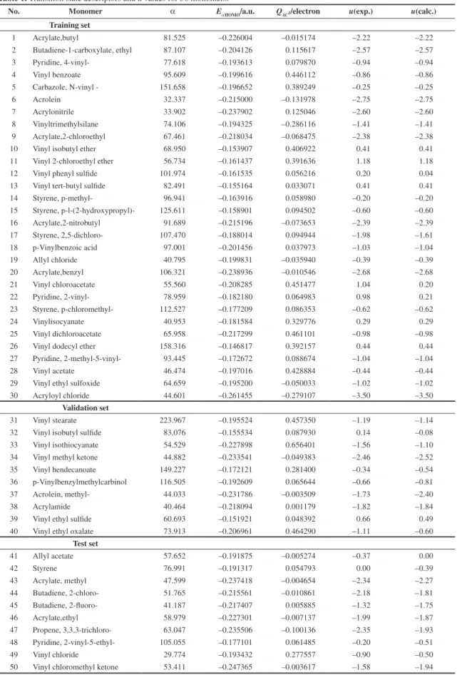
Table 1. Transition state descriptors and u values for 50 monomers.
No. Monomer α EαHOMO/a.u. QAC1/electron u(exp.) u(calc.)
Training set
1 Acrylate,butyl 81.525 –0.226004 –0.015174 –2.22 –2.22
2 Butadiene-1-carboxylate, ethyl 87.107 –0.204126 0.115617 –2.57 –2.57
3 Pyridine, 4-vinyl- 77.618 –0.193613 0.079870 –0.94 –0.94
4 Vinyl benzoate 95.609 –0.199616 0.446112 –0.86 –0.86
5 Carbazole, N-vinyl - 151.658 –0.196652 0.389249 –0.25 –0.25
6 Acrolein 32.337 –0.215000 –0.131978 –2.75 –2.75
7 Acrylonitrile 33.902 –0.237902 0.125046 –2.60 –2.60
8 Vinyltrimethylsilane 74.106 –0.194325 –0.286116 –1.41 –1.41
9 Acrylate,2-chloroethyl 67.461 –0.218034 –0.068475 –2.38 –2.38
10 Vinyl isobutyl ether 68.950 –0.153907 0.406922 0.41 0.41
11 Vinyl 2-chloroethyl ether 56.734 –0.161437 0.391636 1.18 1.18
12 Vinyl phenyl sulfide 101.974 –0.161535 0.056216 0.20 0.04
13 Vinyl tert-butyl sulfide 82.491 –0.155164 0.033071 0.41 0.41
14 Styrene, p-methyl- 96.941 –0.163916 0.058980 –0.20 –0.20
15 Styrene, p-l-(2-hydroxypropyl)- 125.611 –0.158901 0.094502 –0.60 –0.60
16 Acrylate,2-nitrobutyl 91.689 –0.215196 –0.073653 –2.39 –2.39
17 Styrene, 2,5-dichloro- 107.470 –0.188014 0.094944 –1.98 –1.61
18 p-Vinylbenzoic acid 97.001 –0.201456 0.037973 –1.03 –1.04
19 Allyl chloride 40.795 –0.199831 –0.035940 –0.39 –0.39
20 Acrylate,benzyl 106.321 –0.238936 –0.010546 –2.68 –2.68
21 Vinyl chloroacetate 55.560 –0.208285 0.451477 1.04 0.20
22 Pyridine, 2-vinyl- 78.959 –0.182180 0.064983 0.98 0.21
23 Styrene, p-chloromethyl- 112.527 –0.177209 0.086353 –0.62 –0.62
24 Vinylisocyanate 40.953 –0.181584 0.329776 0.29 0.29
25 Vinyl dichloroacetate 65.958 –0.217299 0.461101 –0.98 –0.98
26 Vinyl dodecyl ether 158.316 –0.146817 0.392157 0.44 0.44
27 Pyridine, 2-methyl-5-vinyl- 93.445 –0.172672 0.088674 –1.04 –1.04
28 Vinyl acetate 46.474 –0.197016 0.428884 –0.44 –0.44
29 Vinyl ethyl sulfoxide 64.659 –0.195200 –0.050033 –1.02 –1.02
30 Acryloyl chloride 44.601 –0.261455 –0.279107 –3.50 –3.50
Validation set
31 Vinyl stearate 223.967 –0.195524 0.457350 –1.19 –1.14
32 Vinyl isobutyl sulfide 83.076 –0.155534 0.087930 0.14 –0.08
33 Vinyl isothiocyanate 54.529 –0.227898 0.656401 –1.56 –1.10
34 Vinyl methyl ketone 44.882 –0.233541 –0.049383 –2.46 –2.52
35 Vinyl hendecanoate 149.227 –0.172121 0.281400 –0.34 –0.54
36 p-Vinylbenzylmethylcarbinol 116.505 –0.192609 0.065644 –0.66 –0.81
37 Acrolein, methyl- 44.033 –0.231786 –0.003509 –1.73 –2.40
38 Acrylamide 40.464 –0.218094 0.001179 –1.82 –1.84
39 Vinyl ethyl sulfide 60.693 –0.151921 0.048392 0.66 0.49
40 Vinyl ethyl oxalate 73.913 –0.206961 0.464290 –1.11 –0.60
Test set
41 Allyl acetate 57.652 –0.191875 –0.005274 –0.37 0.00
42 Styrene 76.991 –0.191317 0.054793 0.00 –0.39
43 Acrylate, methyl 47.599 –0.237418 –0.004654 –2.34 –2.27
44 Butadiene, 2-chloro- 51.765 –0.215561 –0.010861 –2.18 –1.81
45 Butadiene, 2-fluoro- 41.187 –0.217407 0.005885 –1.32 –1.75
46 Acrylate,ethyl 58.979 –0.227301 –0.007137 –1.99 –1.87
47 Propene, 3,3,3-trichloro- 63.047 –0.235506 –0.100136 –2.35 –1.93
48 Pyridine, 2-vinyl-5-ethyl- 105.055 –0.177101 0.061485 –0.20 –0.51
49 Vinyl chloride 29.774 –0.193432 0.277557 –0.90 –0.50
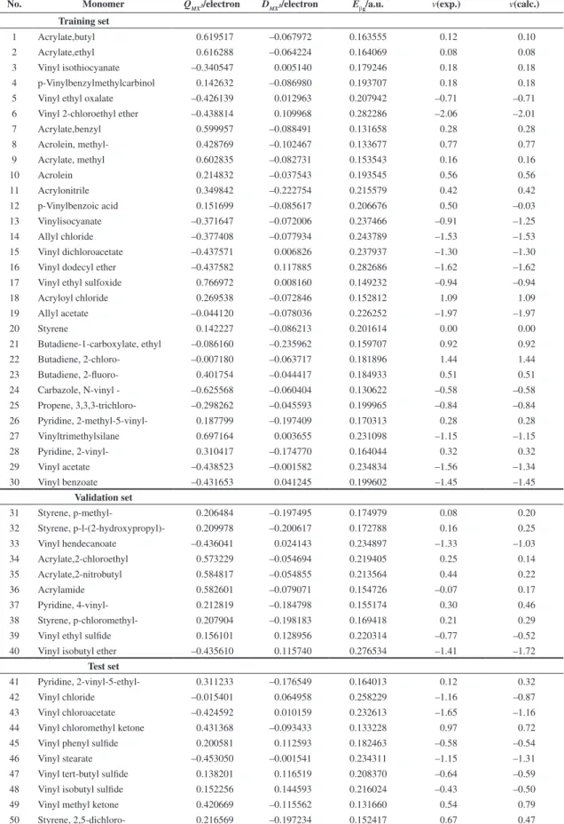
Table 2. Transition state descriptors and v values for 50 monomers.
No. Monomer QMX3/electron DMX3/electron Eβg/a.u. v(exp.) v(calc.)
Training set
1 Acrylate,butyl 0.619517 –0.067972 0.163555 0.12 0.10
2 Acrylate,ethyl 0.616288 –0.064224 0.164069 0.08 0.08
3 Vinyl isothiocyanate –0.340547 0.005140 0.179246 0.18 0.18
4 p-Vinylbenzylmethylcarbinol 0.142632 –0.086980 0.193707 0.18 0.18
5 Vinyl ethyl oxalate –0.426139 0.012963 0.207942 –0.71 –0.71
6 Vinyl 2-chloroethyl ether –0.438814 0.109968 0.282286 –2.06 –2.01
7 Acrylate,benzyl 0.599957 –0.088491 0.131658 0.28 0.28
8 Acrolein, methyl- 0.428769 –0.102467 0.133677 0.77 0.77
9 Acrylate, methyl 0.602835 –0.082731 0.153543 0.16 0.16
10 Acrolein 0.214832 –0.037543 0.193545 0.56 0.56
11 Acrylonitrile 0.349842 –0.222754 0.215579 0.42 0.42
12 p-Vinylbenzoic acid 0.151699 –0.085617 0.206676 0.50 –0.03
13 Vinylisocyanate –0.371647 –0.072006 0.237466 –0.91 –1.25
14 Allyl chloride –0.377408 –0.077934 0.243789 –1.53 –1.53
15 Vinyl dichloroacetate –0.437571 0.006826 0.237937 –1.30 –1.30
16 Vinyl dodecyl ether –0.437582 0.117885 0.282686 –1.62 –1.62
17 Vinyl ethyl sulfoxide 0.766972 0.008160 0.149232 –0.94 –0.94
18 Acryloyl chloride 0.269538 –0.072846 0.152812 1.09 1.09
19 Allyl acetate –0.044120 –0.078036 0.226252 –1.97 –1.97
20 Styrene 0.142227 –0.086213 0.201614 0.00 0.00
21 Butadiene-1-carboxylate, ethyl –0.086160 –0.235962 0.159707 0.92 0.92
22 Butadiene, 2-chloro- –0.007180 –0.063717 0.181896 1.44 1.44
23 Butadiene, 2-fluoro- 0.401754 –0.044417 0.184933 0.51 0.51
24 Carbazole, N-vinyl - –0.625568 –0.060404 0.130622 –0.58 –0.58
25 Propene, 3,3,3-trichloro- –0.298262 –0.045593 0.199965 –0.84 –0.84
26 Pyridine, 2-methyl-5-vinyl- 0.187799 –0.197409 0.170313 0.28 0.28
27 Vinyltrimethylsilane 0.697164 0.003655 0.231098 –1.15 –1.15
28 Pyridine, 2-vinyl- 0.310417 –0.174770 0.164044 0.32 0.32
29 Vinyl acetate –0.438523 –0.001582 0.234834 –1.56 –1.34
30 Vinyl benzoate –0.431653 0.041245 0.199602 –1.45 –1.45
Validation set
31 Styrene, p-methyl- 0.206484 –0.197495 0.174979 0.08 0.20
32 Styrene, p-l-(2-hydroxypropyl)- 0.209978 –0.200617 0.172788 0.16 0.25
33 Vinyl hendecanoate –0.436041 0.024143 0.234897 –1.33 –1.03
34 Acrylate,2-chloroethyl 0.573229 –0.054694 0.219405 0.25 0.14
35 Acrylate,2-nitrobutyl 0.584817 –0.054855 0.213564 0.44 0.22
36 Acrylamide 0.582601 –0.079071 0.154726 –0.07 0.17
37 Pyridine, 4-vinyl- 0.212819 –0.184798 0.155174 0.30 0.46
38 Styrene, p-chloromethyl- 0.207904 –0.198183 0.169418 0.21 0.29
39 Vinyl ethyl sulfide 0.156101 0.128956 0.220314 –0.77 –0.52
40 Vinyl isobutyl ether –0.435610 0.115740 0.276534 –1.41 –1.72
Test set
41 Pyridine, 2-vinyl-5-ethyl- 0.311233 –0.176549 0.164013 0.12 0.32
42 Vinyl chloride –0.015401 0.064958 0.258229 –1.16 –0.87
43 Vinyl chloroacetate –0.424592 0.010159 0.232613 –1.65 –1.16
44 Vinyl chloromethyl ketone 0.431368 –0.093433 0.133228 0.97 0.72
45 Vinyl phenyl sulfide 0.200581 0.112593 0.182463 –0.58 –0.54
46 Vinyl stearate –0.453050 –0.001541 0.234311 –1.15 –1.31
47 Vinyl tert-butyl sulfide 0.138201 0.116519 0.208370 –0.64 –0.59
48 Vinyl isobutyl sulfide 0.152256 0.144593 0.216024 –0.43 –0.50
49 Vinyl methyl ketone 0.420669 –0.115562 0.131660 0.54 0.79
a prescribed parameter of the ε–insensitive loss function, ξ and ξ* are positive slack variables for the data points.
Usually, SVR uses the ε-insensitive loss function to measure the empirical risk (training error):
( ( ) )
( )
( ) ,
( ( ) )
0
f x y f x y
f x y
f x y ε
− ≥ ε
− − ε
− = − < ε
(11)
Thus, Equation 7 can be rewritten as:
*
( ) n( i i) (x )i (x) i
f x =∑ a −a φ ⋅φ +b (12)
where αi and αi
* are the introduced Lagrange multipliers. Through selecting the appropriate kernel function, the entire problem can be solved in the input space itself:
*
( ) s( i i) (x, ) i
f x =∑ a −a K y +b (13)
where s is the number of input data having nonzero values of (αi and αi
*). The kernel function K(.,.) must satisfy the condition of Mercer’s theorem so that it corresponds to some type of inner product in the high-dimensional feature space. In general, the Gaussian radial basis function (RBF) is taken as the kernel function of SVM models:
2
(x , x )i j exp( xi xj )
K = −γ − (14)
The adjustable parameter γ plays a major role in the performance of the kernel, and should be carefully tuned to the problem at hand. So three parameters C, ε and γin ε-SVR models should be adjusted. All SVM models from the present paper were obtained with winSVM (http:// www.cs.ucl.ac.uk/staff/M.Sewell/winsvm/).
Genetic algorithms (GA) are optimization algorithms that mimic natural biological evolution. At each generation, a new set of approximations is created by the process of selecting individuals according to their level of fitness and breeding them together using genetic operators inspired by natural genetics, i.e. random mutation, crossover and selection procedures. This process leads to better models or solutions from an originally random starting population or sample[24,25]. GA together with multiple linear regression (MLR) analysis has become an effective and powerful tool in selecting variables for QSARs. Thus GA-MLR technique in the BuildQSAR program[26] was used in this work. Next, the optimal descriptor sets were used as the input files of SVM models.
The accuracy of a model was evaluated with the root-mean-square (rms) error, which can be expressed as
2
(fi yi) rms
N − ∑
= (15)
where fi is the calculated value, yi is the experimental value for the ith monomer and N is the total number of samples used. The smaller the rms value, the more accuracy the model will be.
Results and Discussion
By analyzing the parameters u and v with respect to the 23 descriptors with the GA-MLR technique in the BuildQSAR program[26], respective optimal subset of descriptors in the model of parameters u
and v was obtained. The optimal subset of descriptors for the parameter u comprises the average molecular polarizability (α), the HOMO energy of alpha spin states (EαHOMO), andAPT charge of C1 atom (Q
AC1). The optimal
descriptor subset for the parameter v consists of Mulliken atomic charge of X3 (Q
MX3), Mulliken atomic spin density
of X3 (D
MX3), and the energy gap between HOMO and
LUMO of beta spin states (Eβg). The values of these descriptors are shown in Tables 1 and 2. The definitions and standardized coefficients of these descriptors in each MLR model are listed in Table 3. A larger absolute value of beta coefficients means the corresponding descriptor is more significant. Thus, EαHOMO and Eβg are the most significant descriptors in the models of parameters u and
v, respectively.
The parameter u denotes the polarity of a monomer. A large u value means less polarity of a monomer. The frontier molecular orbital descriptors, such as EHOMO,
ELUMO, and Eg( = ELUMO - EHOMO) play major roles in governing many chemical reactions[7]. These descriptors were used widely in describing molecular reactivity, stability[27,28], or polarity[7]. According to the frontier molecular orbital theory of chemical reactivity[7], E
HOMO describes the susceptibility of the molecule toward attack by electrophiles and thus is correlated with the ionization potential; and ELUMO, characterizing the susceptibility of the molecule toward attack by nucleophiles, is directly related to the electron affinity. A higher EHOMO value means the stronger electron-donating ability and the smaller electronegativity[2], which results in a smaller electronic effect and molecular polarity. Thus EαHOMO is positively correlated with the parameter u.
Local electron densities or charges are important in many chemical reactions and physicochemical
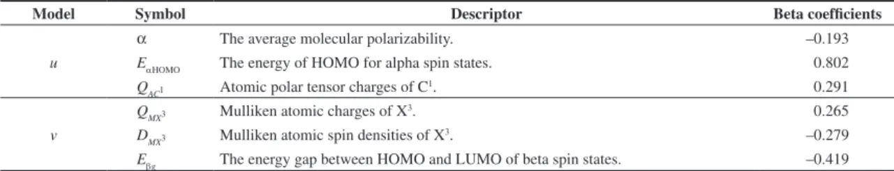
Table 3. Descriptors selected for models, meaning and beta coefficients.
Model Symbol Descriptor Beta coefficients
u
α The average molecular polarizability. –0.193
EαHOMO The energy of HOMO for alpha spin states. 0.802
QAC1 Atomic polar tensor charges of C1. 0.291
v
QMX3 Mulliken atomic charges of X3. 0.265
DMX3 Mulliken atomic spin densities of X3. –0.279
properties of compounds. They are also used widely for the description of the molecular polarity of molecules[7]. Molecular polarity is dependent on bond polarity and the molecular geometry. Generally, for vinyl monomers C1H
2=C
2HR3, the APT charge of C1, Q
AC1 is less than the
charge of C2, Q
AC2. A monomer with the larger descriptor QAC1 suggests that the polar bonds (i.e., the double bond in the monomer) is relatively evenly (or symmetrically) distributed, which results in a less molecular polarity. So it is easy to understand that the descriptor QAC1 is positively related to the parameter u. The last descriptor appearing in the model of u is α, i.e., the average polarizability. α increases with the size of the species either as a result of an increase with the number of electrons or by the expansion of the molecular radius. A large α indicates a large size of substituent group R3 in a vinyl monomer, which may lower the molecular symmetry and lead to a large molecular polarity and a small parameter u. Therefore, α is negatively correlated with the parameter u.
The parameter v describes the intrinsic reactivity of a monomer. A high reactive monomer, that has a large conjugative effect and a large v value, may lower the activation energy gained on adding the radical to the double bond of the monomer. Table 3 shows that v increases with decreasing Eβg. The reason is that a large Eg means high stability for the molecule in the sense of its lower reactivity in chemical reactions[27]. A transition state species (C1H
3– C2HR3• or •C1H
2–C 2H
2R
3) possessing a small E
βg value suggests that the corresponding monomer is prone to forming a transition state structure and has a large parameter
v value. As stated above, atomic charge descriptors can reflect molecular chemical reactivity (or intermolecular interactions)[7]. A large Q
MX3 (Mulliken atomic charge of X
3) or small DMX3 (Mulliken atomic spin density of X3) implies that the monomer is relatively easy to form a transition state structure and has a large v value. Thus, both QMX3 and DMX3 are related to the reactivity parameter v.
The program winSVM was used to develop SVM models for u and v. In order to get satisfactory models, the regularized constant C, the width of the non-penalized tube ε and the bandwidth parameter γ of the RBF kernel function should be selected properly[22]. We take the training of SVM models of u as an example. Firstly, the training set of u (in Table 1) was selected as the input file to obtain 100 models after 100 iterations. The initial optimization results show that a model with SVM parameters of C = 10, ε = 10–4 and γ = 1.0 produced a low rms error. Thus, these SVM parameters were used for further optimization with the validation set. By training the SVM models of u with different γ values of 0.8, 0.9, 1.0, 1.1, 1.2, 1.3, and 1.4 under the condition of C = 10 and ε = 10–4, the validation set produced the rms errors of 0.403, 0.353, 0.327, 0.345, 0.373, 0.390, and 0.405, respectively. Thus, the optimal γ corresponding to the minimal rms error (0.327) was set to 1.0. Subsequently, by applying γ = 1.0 and ε = 10–4, the second parameter C was optimized with C being equal to 7, 8, 9, 10, 11, 12, and 13. The validation set rms errors based on different
C are 0.395, 0.362, 0337, 0.327, 0.328, 0.334, and 0.343, respectively, so the optimal C was equal to 10. Similarly, the third parameter ε under the condition of C of 10 and
γ of 1.0, was optimized with ε = 10–6,ε = 10–5, ε = 10–4, ε = 10–3, ε = 10–2, and ε = 10–1. The validation set rms errors are 0.326, 0.326, 0.327, 0.327, 0.331, and 0.388, respectively. Thus, the optimal ε equals 10–5.
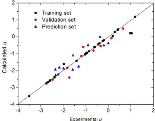
In the end, the optimum ε- SVR model of u with the RBF kernel (C= 10, ε = 10–5 and γ = 1.0) was tested by the prediction set in Table 1. The u values calculated with theoptimal SVR model are listed in Table 1 and depicted in Figure 1. For the SVM model of u, the rms errors for the training, validation and prediction sets are 0.220, 0.326 and 0.345, respectively. The mean rms error and correlation coefficient for 50 monomers are 0.272 and 0.972, respectively.
The three SVM parameters (C, ε and γ) of the model
v were tuned with the same method. Learning parameters of C = 10, ε = 10–4 and γ = 1.0 were selected after initial optimization. Then the different parameters γ (0.9, 1.0, 1.1, 1.2, 1.3, and 1.4), C (5, 10, 15, 20, 25, 30, 35, and 40), and ε (10–6, 10–5, 10–4, 10–3, 10–2 and 10–1), were tested successively. Respective validation set rms errors are 0.271, 0.254, 0.242, 0.236, 0.254, and 0.272 for different γ values (C = 10 and ε = 10–4); 0.337, 0.236, 0.214, 0.206, 0.206, 0.216, 0.241, and 0.289 for different
C values (γ = 1.2 and ε = 10–4); and 0.206, 0.206, 0.206,
Figure 2. Plot of the experimental versus calculated v values.
0.206, 0.212, and 0.254 for different ε values (C = 20 and γ = 1.2). Thus, the optimal SVM parameters for v should be C = 20, γ = 1.2 and ε = 10–4.
The optimal ε-SVR model for v produced rms errors for the training set of 0.123, the validation set of 0.206 and the prediction set of 0.238. The mean rms error and correlation coefficient for the parameter v of 50 monomers are 0.170 and 0.981, respectively, which are comparable to the values of existing models[12]. The calculated v valuesfrom the optimal SVR model are listed in Table 2 and depicted in Figure 2.
It should be noted that there are significant experimental errors for reactivity parameters such as
Q, e, u, and v. For example, as long as the correlation coefficient R between the experimental and calculated e
values is greater than 0.876 (rms = 0.326), then a good fit has been achieved[2,12]. This means these QSAR models of reactivity parameters (u and v) are acceptable if their correlation coefficients are close to or above 0.9. Our models in this paper have correlation coefficients of 0.972 for u and 0.981 for v, denoting that our results for the model e are satisfactory and acceptable.
Conclusions
QSAR models of the reactivity parameters u and v
in the U-V scheme used for the prediction of reactivity ratios and transfer constants for vinyl monomers in radical copolymerization were developed, by applying GA and SVM techniques. Quantum chemical descriptors used to build SVR models, were calculated from transition state species with structures C1H
3–C
2HR3• or •C1H 2–C
2H 2R
3, formed from vinyl monomer C1H
2=C
2HR3 + H•. The models were proved to be accurate with mean rms errors of 0.272 (R = 0.972) for u and 0.170 (R = 0.981) for v, which demonstrate that calculating descriptors from transition state structures to develop SVM models for reactivity parameters u and v is feasible.
Acknowledgements
This work was financially supported by the National Natural Science Foundation of China (no. 20972045), the Hunan Provincial Natural Science Foundation of China (no. 12JJ6011) and the Science Foundation of Hunan Province (no. 2010FJ4116)
References
1. Jenkins, A. D. & Jenkins, J. - Macromol. Symp., 174, p.187 (2001). http://dx.doi.org/10.1002/1521-3900(200109)174:1%3C187::AID-MASY187%3E3.0.CO;2-4 2. Zhan, C. G. & Dixon, D. A. - J. Phys. Chem. A, 106,
p.10311 (2002). http://dx.doi.org/10.1021/jp020497u 3. Jenkins, A. D. - J. Polym. Sci. Part A: Polym. Chem., 37,
p.113 (1999). http://dx.doi.org/10.1002/(SICI)1099-0518(19990115)37:2%3C113::AID-POLA1%3E3.0.CO;2-C 4. Alfrey, T. & Price, C. C. – J. Polym. Sci., 2, p.101 (1947).
http://dx.doi.org/10.1002/pol.1947.120020112
5. Jenkins, A. D.; Hatada, K.; Kitayama, T. & Nishiura, T. - J. Polym. Sci. Part A: Polym. Chem., 38, p.4336 (2000). http://dx.doi. org/10.1002/1099-0518(20001215)38:24%3C4336::AID-POLA20%3E3.0.CO;2-4
6. Brandrup, J.; Immergut, E. H. & Grulke, E. - “Polymer Handbook”, 4th ed., Wiley, New York (1999).
7. Karelson, M.; Lobanov, V. S. & Katritzky, A. R. - Chem. Rev., 96, p.1027 (1996). http://dx.doi.org/10.1021/cr950202r 8. Yu, X. L.; Wang, X. Y.; Gao, J. W.; Li, X. B. & Wang, H.
L. - Polymer, 46, p.9443 (2005). http://dx.doi.org/10.1016/j. polymer.2005.07.039
9. Ivanciuc, O. - Internet Electron. J. Mol. Des. 1, p.269 (2002). 10. Xu, J.; Wang, L.; Wang, L. X.; Shen, X. L. & Xu, W.
L. - J. Comput. Chem., 32, p.3241 (2011). http://dx.doi. org/10.1002/jcc.21907
11. Xu, J.; Chen, B.; Zhang, Q. & Guo, B. - Polymer, 45, p.8651 (2004). http://dx.doi.org/10.1016/j.polymer.2004.10.057 12. Yi, B.; Tan, Z. D. & Yu, X. L. - Chin. J. Chem., 29, p.41
(2011). http://dx.doi.org/10.1002/cjoc.201190058 13. Dossi, M.; Liang, K.; Hutchinson, R. A. & Moscatelli,
D. - J. Phys. Chem. B, 114, p.4213 (2010). http://dx.doi. org/10.1021/jp1007686
14. Yu, X. L.; Liu, W. Q.; Liu, F. & Wang, X. Y. - J. Mol. Model., 14, p.1065 (2008). http://dx.doi.org/10.1007/s00894-008-0339-3 15. Yu, X. L.; Yi, B. & Wang, X. Y. - Eur. Polym. J., 44, p.3997
(2008). http://dx.doi.org/10.1016/j.eurpolymj.2008.09.028 16. Yu, X. L.; Wang, X. Y. & Li, B. - Colloid. Polym. Sci., 288,
p.951 (2010). http://dx.doi.org/10.1007/s00396-010-2215-9 17. Cioslowski, J. - J. Am. Chem. Soc., 111, p.8333 (1989).
http://dx.doi.org/10.1021/ja00204a001
18. Chelani, A. B. - Environ. Monit. Assess., 162, 169 (2010). http://dx.doi.org/10.1007/s10661-009-0785-0
19. Camps-Valls, G.; Chalk, A. M.; Serrano-López, A. J. Martín-Guerrero, J. D. & Sonnhammer, E. L. - BMC Bioinformatics, 5, p.135 (2004). http://dx.doi. org/10.1186/1471-2105-5-135
20. Pourbasheer, E.; Riahi, S.; Ganjali, M. R. & Norouzi, P. – Eur. J. Med. Chem., 44, p.5023 (2009). http://dx.doi. org/10.1016/j.ejmech.2009.09.006
21. Yu, X. L.; Wang, X. Y. & Chen, J. F. - J. Chil. Chem. Soc., 56, p.746 (2011). http://dx.doi.org/10.4067/S0717-97072011000300006
22. Yu, X. L.; Yi, B.; Wang, X. Y. & Chen, J. F. - Atmos. Environ., 51, p.124 (2012). http://dx.doi.org/10.1016/j. atmosenv.2012.01.037
23. Darnag, R.; Mazouz, E. L. M.; Schmitzer, A.; Villemin, D.; Jarid, A. & Cherqaoui, D. – Eur. J. Med. Chem., 45, p.1590 (2010). http://dx.doi.org/10.1016/j.ejmech.2010.01.002 24. Eiben, E.; Hinterding, R. & Michalewicz, Z. - IEEE
Trans. Evol. Comput., 3, p.124 (1999). http://dx.doi. org/10.1109/4235.771166
25. Turabekova, M. A. & Rasulev, B. F. - Molecules, 9, p.1194 (2004). http://dx.doi.org/10.3390/91201194
26. De Oliveira, D. B. & Gaudio, A. C. - Quant. Struct.-Act. Relat., 19, p.599 (2000). http://dx.doi.org/10.1002/1521-3838(200012)19:6%3C599::AID-QSAR599%3E3.0.CO;2-B 27. Zhou, Z. & Parr, R. G. - J. Am. Chem. Soc., 112, p.5720
(1990). http://dx.doi.org/10.1021/ja00171a007
28. Yu, X. L.; Yu, W. H.; Yi, B. & Wang, X. Y. - Collect. Czech. Chem. Commun., 74, p.1279 (2009). http://dx.doi. org/10.1135/cccc2008215