(*) This research is part of a project sponsored by the Fundação de Ciência e Tecnologia do Ministério de Ciência e Tecnologia, Portugal, reference: PTDC/ECO/72065/2006. We would like to thank Rui M. Pereira for very useful comments and suggestions.
December 2010
Final energy demand in Portugal:
How persistent it is and why it matters for environmental policy
(*)
Alfredo Marvão Pereira
Department of Economics, College of William and Mary, Williamsburg, VA, USA Center for Advanced Studies in Economics and Econometrics - CASEE, Portugal
Email: [email protected]
José Manuel Belbute
Department of Economics, University of Évora, Portugal
Center for Advanced Studies in Management and Economics - CEFAGE, Portugal Email: [email protected]
Abstract
The objective of this paper is to analyze the degree of persistence of final energy demand in Portugal. Our results suggest the presence of a strong level of persistence for aggregate final energy demand. Final demand for gas is the most persistent component of energy demand, while the final demand for coal is the least persistent. In turn, final demand for petroleum and biomass tend to have levels of persistence similar to aggregate final demand. The case of final demand for electricity is inconclusive. These results have the important implication for the design of environmental policies. First, the fact that final energy demand is highly persistent is good news in that environmental policies in Portugal can be implemented in a favorable setting in which their effects will tend to be long lasting. Second, the high persistence of gas and the fact that biomass and petroleum have levels of persistence that are similar suggests that fuel switching policies will be relatively easy to implement in these cases. The case of coal is somewhat different in that switching away from coal may not be easy. In turn, the case of electricity is somewhat ambiguous. While the fact that it is also highly persistent suggests that shocks to its final demand will produce long lasting effects, it is not clear, however, how they compare to the effects on the other final demand components and therefore we can make no statements about fuel switching. Keywords: Persistence, final energy demand, fuel switching, environmental policy, Portugal. JEL Codes: C14, C22,O13, Q41.
1
Final energy demand in Portugal:
How persistent it is and why it matters for environmental policy
1. Introduction
The objective of this paper is to address the issue of the degree of persistence in final energy demand in Portugal and to identify its implications for environmental policy. Persistence can be thought of as a measure of the speed at which a variable returns to its baseline after a shock. In this sense, when the degree of persistence is small, a shock tends to have more temporary effects and conversely when the degree of persistence is high, a shock tends do have more long-lasting effects.
Identifying the degree of persistence in final energy demand is important from an environmental policy perspective, as climate change is essentially and energy issue. Exogenous shocks to types of energy demand with large degrees of persistence have a long lasting impact while types of energy demand with a low degree of persistence do not respond in a durable way to exogenous shocks. Intuitively, it is more costly and more difficult to permanently affect energy demand when persistent is low. Policy shocks designed, for example, to reduce carbon emissions will have long lasting effects if final energy demand is persistent. In addition, it is easier to reduce final energy demand for types of energy that show higher degrees of persistence since a single negative shock to such variables will generate a reduction in consumption that will last longer. As a corollary, the degree of persistence of final energy demand will make a difference as to the effectiveness of environmental policies that promote either energy efficiency or fuel switching.
Naturally, the issues of energy efficiency and fuel switching assume front stage in the current debate. Environmental policies have been traditionally centered on investment in research, development and deployment of energy-efficient technologies, on restructuring the composition of fuel demand, and on reducing energy consumption. The simple reduction of energy consumption is a difficult matter in particular for developing countries. Energy-efficiency improvements have the potential for bringing significant gains in productivity while reducing the consumption of fossil fuels and greenhouse gas emissions. Nevertheless, their scope is rather limited. The development of energy-efficient technologies is more of a long-term prospect and more outside the scope of small or developing economies. Ultimately, policy instruments that promote fuel switching tend to be the policies of choice.
2
Identifying the degree of persistence of the relevant variables is a well-established concern in the macroeconomic literature. A primary example is the case of the analysis of inflation persistence [see, for example, Willis (2003), Gadzinsky and Orlandi (2004), Levin and Piger (2004), Marques (2004), Piveta and Reis (2007), Cogley et al. (2008), and Dias & Marques (2010)]. Other areas include, for example, the investigation of persistence in aggregate output or the deviations of the economy from purchasing power parity conditions and the connection between wage and price setting and persistence.
One common feature of this literature is the use of scalar measures of persistence. These have the advantage of summarizing in a convenient manner the information contained in the impulse response functions of the estimated data generating process for the variable in question. The use of a scalar indicator is particularly useful in comparing the degree of persistence across series. The most popular scalar indicator of persistence, in particular, in the inflation persistence literature, is the use of sum of the autoregressive coefficients. Other commonly used scalar measures of persistence include the largest autoregressive root, the spectrum at zero frequency, or the half-life decay [see Marques (2004) for a discussion on the relative merits of these different measures].
In this paper we measure persistence in final energy demand in Portugal by using the sum of autoregressive coefficients. In addition, we use the non-parametric scalar measure of persistence introduced in Marques (2004) and Dias and Marques (2010). This new scalar measure of persistence is based on the idea that persistence and mean reversion are inversely related and is defined as the unconditional probability of a stationary stochastic process not crossing its mean at any given period t. This measure of persistence has the advantage of not requiring the specification and the estimation of the data generating process for the series. Furthermore, by focusing on mean reversion this measure of persistence highlights the relevance of accounting for changes in the mean of the series, as failure to do so would result in a spurious higher measurement of persistence, i.e., the measure of persistence is spuriously maximized by assuming that the series has a time invariant mean.
This paper is closely related to the energy literature on unit roots and long memory properties of energy consumption [see Hsu et al (2008) for an overview of this literature]. This literature has focused on the issue of the stationarity using univariate unit roots tests with or without consideration of structural breaks [see, for example, Altinay and Karagol (2004), Lee and Chang (2005), and Narayan and Smyth (2005)]. More recently, and due to the mixed empirical evidence and the concern with the low power of the univariate tests, the focus has been on the use of panel unit root tests again with or without the consideration of structural breaks
3
[see, for example, Al-Iriani (2006), Chen and Lee (2007), Hsu et al (2008), Lee (2005), Lee and Chang (2008), Narayan and Smyth (2007), and Mishra et al (2009)].
Overall the energy literature on unit roots and long memory properties, in particular in recent years, has focused almost invariably on total energy consumption and on Asia and Pacific region countries. Moreover, and more importantly from a policy perspective, the issue of long memory has been addressed as an all or nothing proposition under the usual dichotomy of the stationary/non-stationary cases. Recent exceptions are Lean and Smyth (2008) and Gil-Alana, Payne, and Loomis (2010) which focus respectively on petroleum consumption and energy consumption of the electric power sector in the US in the context of fractional integration. The absence of evidence on the degree of persistence of final energy demand using more flexible measures of persistence, allowing for a more disaggregated level, and focusing in more advanced economies is an important void in the literature. This is a void that we are starting to fill with this paper by concentrating on the case of final energy demand in Portugal and by considering not only final energy demand but also its major components. Furthermore, our use of scalar measures of persistence makes it possible to make comparisons across different types of energy demand and opens the door to identifying the policy implications of the finding not only in terms of energy efficiency policies but also fuel switching.
The paper is organized as follows. Section 2 presents the data set. Section 3 presents the empirical evidence on persistence using standard parametric tests while section 4 does the same using non-parametric tests. Section 5 discusses the evidence on changes in the patterns of persistence for different sub-samples. Finally, section 6 provides a summary of the results and discusses their policy implications.
2. Data: sources and description
We use annual data for final energy demand for the period 1977 to 2003. Data was obtained from the Energy Balance Sheets published by Direcção Geral de Energia (Portuguese Department of Energy, DGE hereafter). Aggregate final demand for energy is defined as the sum of five final demand components: petroleum and its derivatives, coal, gas, biomass, and electricity. All variables are measured in 103 tons of oil equivalent (toe hereafter).
In 1990, the DGE changed its data collection methodology in order to better reflect the distinction between primary and final energy demand. As a result, the DGE makes available two data sets – one for the period between 1971 and 1993 and another for the period between 1990 and 2003 - with a four-year overlap. The data collection methodology and
4
presentation differs significantly between the two periods and to ensure consistency between the two series, several methodological issues are taken into consideration as detailed below. Final demand for petroleum and its derivatives includes liquefied petroleum gas, gasoline, diesel and fuel oil. Although the dominant use of petroleum and its derivates is as an energy source, they are also used as raw materials in the production of, for example, plastics and asphalt. Petroleum derivatives used as raw materials are not considered in our data, with the exception of fuel oil. This is because prior to 1985 the DGE methodology did not distinguish between fuel oil used for energy and non-energy purposes. Petroleum and its derivatives account for 66.3% of final energy demand for the sample period and show a declining trend from 69.6% between 1977 and 1985 to 63.9% in the final years of the sample period.
Final demand for coal includes domestic production and imports of anthracite and bituminous coal. This data set is rather consistent methodologically throughout the sample period and therefore no adjustments to the published data were necessary. Coal constitutes 4.5% of total final energy demand for the sample period. Its weight in total final energy consumption has shown some fluctuations, starting at 3.9% in the beginning of the sample period reaching a high of 6.0% for 1986 to 1997 and decreasing to 2.1% in the last five years of the sample period. The virtual extinction of the domestic coal mining industry - the last coal mine in Portugal producing primarily low grade anthracite closed in 1994 - largely contributed to the steady decline in coal consumption, particularly after 1998.
Final demand for gas includes coke gas, blast furnace gas, city gas and natural gas. Natural gas distribution infrastructure developed rapidly after 1998 to become an important component of the energy system in Portugal. The demand for gas itself has increased significantly with the introduction of natural gas. In fact, the average share of gas in total final energy consumption for the period 1977-1985 was 1.2% and rose to 5.8% between 1998 and 2003. Gas consumption grew, on average, at an average annual rate of 25.9% after the introduction of natural gas in 1998. In our empirical analysis below we fully consider the possibility of a structural break in 1998 consistent with the introduction of natural gas.
Final demand for biomass includes registered purchases up until 1993, after which, data is based upon household surveys and thus reports both purchases and collection of biomass and forest waste. In order to generate a consistent series in levels, the growth rate of biomass consumption after 1990 is applied to the earlier level data. We find that the implied growth rate during the overlapping period 1990-1993 is consistent, albeit with relatively insignificant deviations. The use of biomass has decreased in relative importance over the sample period.
5
Between 1977 and 1985, biomass consumption represents 8.7% of total final energy demand while in the final years of the sample period accounts for only 6.1%.
Final demand for electricity includes cogeneration and heat until 1993, after which they are accounted for separately. The level values for the overlapping years of 1990 - 93 show an average variation of 1.04% between the two samples, the growth rates show larger variability in the order of 20%. As such we consider level data for electricity generation until 1993 after which the new data in growth rates is considered to extend this series. Electricity demand has grown in relative importance. It represents 16.6% of total final energy demand between 1977 and 1985 and 22.0% for the last years of the sample period.
3. On the degree of persistence of final energy demand: a parametric approach 3.1 Methodology
Persistence of a stationary time series can be defined as the speed at which a variable returns to its equilibrium or its long-run level after a shock. The implication of this definition is that any change in a time series tends to be temporary if the series exhibit a low degree of persistence whereas a shock will have long-lasting effects on a (more) persistent time series.
The usual way to capture the degree of persistence is by the estimation of the sum of the
autoregressive coefficient. In our case, this methodology consists in using the residuals of the
appropriate regression models and estimating 𝜌 using
𝜖𝑡= 𝛿𝑗∆𝜖𝑡−𝑗+ 𝜌𝜖𝑡−1+ 𝜀𝑡
𝑝−1
𝑗 =1
(1)
where 𝜖𝑡 represents the residuals from the models in Table 3.
The parameter 𝜌 corresponds to the sum of the auto-regressive coefficients and provides an estimate for the level of persistence associated with each type of energy demand. The coefficient of persistence varies between 0 and 1 and larger values indicate a greater degree of persistence in the variable.
6
We start by addressing the issue of the stationarity of the different energy demand series. The unit root literature shows that the existence of structural breaks can qualitatively affect the robustness and nature of the results of the standard stationarity tests. Accordingly, we consider the possibility of structural breaks in the times series under analysis that affect their deterministic components. Since we have very good priors at to the possible break points we start with the case of known structural breaks
We use the Chow test to confirm the dates of the expected structural breaks. A structural break in the series for aggregate final energy demand, petroleum and biomass is identified in 1986, consistent with the date in which Portugal joined the European Union. Final demand for coal and gas show a structural break in 1998 consistent with the introduction of natural gas in Portugal. A structural break in 1993 was identified for the electricity series which is the date in which the two series available from the DGE were combined.
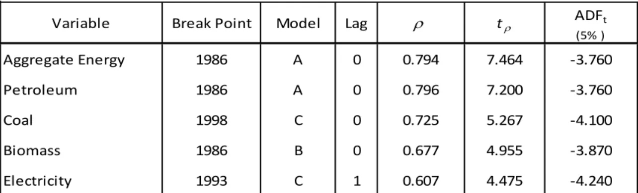
Now that the dates for the structural breaks have been confirmed, we test for the existence of unit roots in the "noise function" using the test proposed by Perron (1989). This test considers three deterministic functions corresponding to three models that test the possibility of changes in the mean (Model A – crash model), in the trend (Model B – growth model), and in both (Model C – crash and growth model). Table 1 presents the results of the unit root tests with known break points. When a series shows evidence of trend stationarity in two of the three models, we consider the model with the lowest BIC. Our test results suggest that, all series except final demand for gas are stationary.
It should be mentioned that although the unit root test results are in general very robust, the evidence of non-stationarity for gas does not seem to be very robust. Indeed, when we consider separately the two sub samples before and after 1998, we find that the first subsample is unambiguously trend stationary with a quadratic trend and that the second sub-sample is also trend stationary when using the KPSS test [see Kwiatkowski et al. (1992)]but not with the DF-ADF test [see Eliot et al. (1996)].Furthermore, the Zivot-Andrews (1998) test of unit roots with an unknown break point suggests that gas is stationary with 1997 as the most likely timing for the break.
7
Model A - Change in the mean; Model B - Change in the trend; Model C - Change in both
Figure 1 – Actual and de-trended values: the parametric case
a)Aggregate energy b) Petroleum c) Coal
d) Biomass e) Electricity
3.3 Persistence results
The results in Table 1 suggest that aggregate final energy demand is highly persistent with 𝜌 = 0.794. This closely mirrors the value of 𝜌 for final demand for petroleum, which accounts for approximately 2/3 of total final energy demand in Portugal. The persistence levels for coal, biomass and electricity are lower but still high. Furthermore, we can reject at the 5% level the null hypothesis of equality in the level of persistence between aggregate energy demand or petroleum and its derivatives and electricity demand.
4e+006 6e+006 8e+006 1e+007 1.2e+007 1.4e+007 1.6e+007 1980 1985 1990 1995 2000 tt Efectivo e ajustado tt ajustado efectivo 4e+006 5e+006 6e+006 7e+006 8e+006 9e+006 1e+007 1.1e+007 1980 1985 1990 1995 2000 pt Efectivo e ajustado pt ajustado efectivo 100000 200000 300000 400000 500000 600000 700000 800000 1980 1985 1990 1995 2000 ct Efectivo e ajustado ct ajustado efectivo -1e+006 -800000 -600000 -400000 -200000 0 200000 400000 600000 800000 1e+006 1980 1985 1990 1995 2000 umodAtt -1.2e+006 -1e+006 -800000 -600000 -400000 -200000 0 200000 400000 600000 1980 1985 1990 1995 2000 umodApt -300000 -250000 -200000 -150000 -100000 -50000 0 50000 100000 150000 200000 1980 1985 1990 1995 2000 resíduo
Resíduos de regressão (= observados - ajustados ct)
500000 550000 600000 650000 700000 750000 800000 850000 900000 950000 1e+006 1980 1985 1990 1995 2000 bt Efectivo e ajustado bt ajustado efectivo 500000 1e+006 1.5e+006 2e+006 2.5e+006 3e+006 3.5e+006 4e+006 1980 1985 1990 1995 2000 et Efectivo e ajustado et ajustado efectivo -150000 -100000 -50000 0 50000 100000 150000 1980 1985 1990 1995 2000 umodBbt -80000 -60000 -40000 -20000 0 20000 40000 60000 80000 1980 1985 1990 1995 2000 zCet
Variable Break Point Model Lag r tr ADFt
(5% ) Aggregate Energy 1986 A 0 0.794 7.464 -3.760 Petroleum 1986 A 0 0.796 7.200 -3.760 Coal 1998 C 0 0.725 5.267 -4.100 Biomass 1986 B 0 0.677 4.955 -3.870 Electricity 1993 C 1 0.607 4.475 -4.240
8
Finally, the evidence of a unit root for gas suggests a very high level of persistence and a very long memory response to shocks. As we discussed in the previous section, however, the result of non-stationarity for gas does not seem to be very robust. We are left with some evidence for a long memory but also some mixed evidence opening the door to the possibility of stationarity. Accordingly, the non-parametric results may be particularly informative in the case of final demand for gas.
4. On the level of persistence of the final energy demand: a non-parametric approach 4.1 Methodology
Recently, Marques (2004) and Dias & Marques (2010) suggested the use of a non-parametric method for quantifying the level of persistence. This approach is based on the relationship between persistence and the concept of mean reversion. The measure of persistence 𝛾can be defined as the unconditional probability of a stationary stochastic process not crossing its mean at time t
𝛾 = 1 −𝑛
𝑇 (2)
where n stands for the number of times the series crosses the mean during a time interval with
T + 1 observations. The ratio n/T itself gives the degree of mean reversion.
By definition, this indicator of persistence varies between 0 and 1. In the context of a symmetric white noise process with mean zero, the case of 𝛾 = 0.5 corresponds to the absence of significant persistence. When 𝛾 > 0.5 we find evidence of greater persistence and with values below 0.5 we find evidence of negative autocorrelation.
The advantage of this approach is that it does not require any assumptions with respect to the data generating process but rather extracts the deterministic component of the series using appropriate methods. In addition, this approach is also robust to the presence of outliers in the data and is particularly well suited for cases of changing deterministic components. Naturally, the non-parametric test results are sensitive to the method used to de-trend the data series. The non-parametric estimation that follows considers two possibilities in terms of de-trending that is, in terms of extracting the mean for the different data series. In both cases we consider the presence of a variable long term trend in the mean for the series. First, we consider the crash and growth case where the structural breaks cause a mean shift and a change in the growth rate. The second approach consists in extracting cyclical components by application of the Hodrick-Prescott filter.
9
4.2 Non-parametric persistence tests using crash and growth effects
In this section we use the residuals from a crash and growth model as in Perron (1989) to extract the time varying mean of the different variables and thereby determine the level of persistence for final energy demand. The basic model is
𝜀𝑡= 𝑦𝑡− 𝜇0+ 𝛿0𝑡 + 𝜇1𝐷𝑡+ 𝛿1𝑡𝐵 (3)
where 𝑡𝐵 is a dummy variable that assumes the value of 1 for 𝑡 > 𝑇𝐵 (in which 𝑇𝐵 is the time of the break) and zero otherwise. This dummy variable models the effect of the crash on the mean. 𝐷𝑡 is another dummy which interacts with the time trend that assumes the value of 𝑡 for 𝑡 > 𝑇𝐵 and zero otherwise. This term model the impact on the growth rate of the mean. The results are presented in Table 2 and Figure 2.
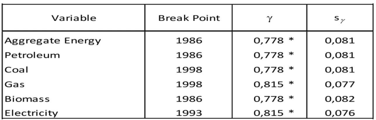
Test results confirm the presence of a strong degree of persistence in aggregate and disaggregate final energy demand, in that in all cases the null hypothesis of the absence of persistence can be rejected at the 5% level. Furthermore, we also reject at the 5% level the null hypothesis of equality in persistence levels between gas and electricity on one hand and the remaining components on the other hand. Specifically, gas and electricity present larger levels of persistence than the remaining components of final energy demand.
Table 2 – Non-Parametric evaluation of persistence: crash and growth effects
Variable Break Point
Aggregate Energy 1986 0,778 * 0,081 Petroleum 1986 0,778 * 0,081 Coal 1998 0,778 * 0,081 Gas 1998 0,815 * 0,077 Biomass 1986 0,778 * 0,082 Electricity 1993 0,815 * 0,076 sg g
* Stands for the rejection of the null of g = 0.5 (absence of persistence)
10
a)Aggregate energy b) Petroleum c) Coal
e) Gas f) Biomass g) Electricity
4.3 Non-parametric persistence tests using the Hodrick-Prescott filter
Another approach to extracting the mean of aggregate final energy demand and of its five components consists in using a pure statistical model and the Hodrick-Prescott (1981) filter. This is a well known method to obtain the smoothed non-linear representation of a time series. Formally, the trend or mean component of the time series 𝜇𝑡 is the solution to
: min 𝜇𝑡 𝑦𝑡− 𝜇𝑡 2 𝑇 𝑡=1 + 𝜆 𝜇𝑡+1− 𝜇𝑡 − 𝜇𝑡− 𝜇𝑡−1 2 𝑇−1 𝑡=2 (4)
i.e., this filter seeks to minimise the cyclical component 𝑦𝑡− 𝜇𝑡 subject to a smoothness condition reflected in the second term. The second term penalizes variations in the growth rate of the trend component. The larger the value of λ, the higher is the penalty and thus the smoother will be the trend. In the limit, as goes to infinity, the filter will choose a linear trend while if
0
it recovers the original series. A simple and common way to set the value of is at 100 times the square of the data frequency. Given that our data is of annual frequency we set = 100. Results are presented in Table 3 and Figure 3.6e+006 7e+006 8e+006 9e+006 1e+007 1.1e+007 1.2e+007 1.3e+007 1.4e+007 1.5e+007 1.6e+007 1.7e+007 1980 1985 1990 1995 2000 tt Efectivo e ajustado tt ajustado efectivo 4e+006 5e+006 6e+006 7e+006 8e+006 9e+006 1e+007 1.1e+007 1980 1985 1990 1995 2000 pt Efectivo e ajustado pt ajustado efectivo 100000 200000 300000 400000 500000 600000 700000 800000 1980 1985 1990 1995 2000 ct Efectivo e ajustado ct ajustado efectivo -800000 -600000 -400000 -200000 0 200000 400000 600000 800000 1980 1985 1990 1995 2000 umodCtt -500000 -400000 -300000 -200000 -100000 0 100000 200000 300000 400000 1980 1985 1990 1995 2000 resíduo
Resíduos de regressão (= observados - ajustados pt)
-300000 -250000 -200000 -150000 -100000 -50000 0 50000 100000 150000 200000 1980 1985 1990 1995 2000 resíduo
Resíduos de regressão (= observados - ajustados ct)
0 200000 400000 600000 800000 1e+006 1.2e+006 1.4e+006 1980 1985 1990 1995 2000 gt Efectivo e ajustado gt ajustado efectivo 550000 600000 650000 700000 750000 800000 850000 900000 950000 1e+006 1980 1985 1990 1995 2000 bt Efectivo e ajustado bt ajustado efectivo 500000 1e+006 1.5e+006 2e+006 2.5e+006 3e+006 3.5e+006 4e+006 1980 1985 1990 1995 2000 et Efectivo e ajustado et ajustado efectivo -100000 -50000 0 50000 100000 150000 200000 1980 1985 1990 1995 2000 resíduo
Resíduos de regressão (= observados - ajustados gt)
-60000 -40000 -20000 0 20000 40000 60000 80000 100000 1980 1985 1990 1995 2000 resíduo
Resíduos de regressão (= observados - ajustados bt)
-80000 -60000 -40000 -20000 0 20000 40000 60000 80000 1980 1985 1990 1995 2000 zCet
11
Test results confirm the existence of persistence in aggregate energy demand and in its components. Final demand for coal presents an exception to these results, in that we find a statistically significant absence of persistence. This suggests that the response of coal demand to exogenous shocks is quick and the effects of such shocks are temporary. In addition, we fail to reject at the 5% level the null hypothesis of equality in persistence for the final demand for electricity on one hand and biomass, petroleum or aggregate final energy demand on the other hand.
Table 3 – Non-parametric evaluation of persistence: the Hodrick-Prescott filter
Variable Break Point
Aggregate Energy 1986 0,778 * 0,081 Petroleum 1986 0,778 * 0,081 Coal 1998 0,593 0,097 Gas 1998 0,889 * 0,062 Biomass 1986 0,778 * 0,082 Electricity 1993 0,741 * 0,086 sg g
* Stands for the rejection of the null of g = 0.5 (absence of persistence)
Figure 3 – Actual and de-trended values: the Hodrick-Prescott filter
a)Aggregate energy b) Petroleum c) Coal
d) Gas e) Biomass f) Electricity
Finally, we reject at the 5% level the null hypothesis of equal persistence between gas and the other components of the final demand for energy. Specifically, gas shows a statistically higher degree of persistence than the rest of the final energy demand components. The estimated
6e+006 7e+006 8e+006 9e+006 1e+007 1.1e+007 1.2e+007 1.3e+007 1.4e+007 1.5e+007 1.6e+007 1.7e+007 1975 1980 1985 1990 1995 2000 2005 tt (dados originais) tt (alisados) -600000 -400000 -200000 0 200000 400000 600000 1975 1980 1985 1990 1995 2000 2005 Componente cÃ-clica de tt 4e+006 5e+006 6e+006 7e+006 8e+006 9e+006 1e+007 1.1e+007 1975 1980 1985 1990 1995 2000 2005 pt (dados originais) pt (alisados) -500000 -400000 -300000 -200000 -100000 0 100000 200000 300000 400000 1975 1980 1985 1990 1995 2000 2005 Componente cÃ-clica de pt 100000 200000 300000 400000 500000 600000 700000 800000 1975 1980 1985 1990 1995 2000 2005 ct (dados originais) ct (alisados) -200000 -150000 -100000 -50000 0 50000 100000 150000 1975 1980 1985 1990 1995 2000 2005 Componente cÃ-clica de ct 0 200000 400000 600000 800000 1e+006 1.2e+006 1.4e+006 1975 1980 1985 1990 1995 2000 2005 gt (dados originais) gt (alisados) -250000 -200000 -150000 -100000 -50000 0 50000 100000 150000 200000 1975 1980 1985 1990 1995 2000 2005 Componente cÃ-clica de gt 550000 600000 650000 700000 750000 800000 850000 900000 950000 1e+006 1975 1980 1985 1990 1995 2000 2005 bt (dados originais) bt (alisados) -80000 -60000 -40000 -20000 0 20000 40000 60000 80000 100000 1975 1980 1985 1990 1995 2000 2005 Componente cÃ-clica de bt 500000 1e+006 1.5e+006 2e+006 2.5e+006 3e+006 3.5e+006 4e+006 1975 1980 1985 1990 1995 2000 2005 et (dados originais) et (alisados) -80000 -60000 -40000 -20000 0 20000 40000 60000 80000 1975 1980 1985 1990 1995 2000 2005 Componente cÃ-clica de et
12
inertia for gas constitutes an interesting and paradigmatic case since until 1998 with the introduction of natural gas, final demand for gas consisted of gas derived from solid fuels. Until 1998, the series for gas showed asmooth evolution through time with a mild growth in the mean. With the introduction of natural gas in 1998 the demand for gas grew by 1000% in 3 years. The high degree of persistence in the demand for gas shows its enormous capacity to remain tight with its trend, despite the significant and abrupt growth in such a short time due to growth in natural gas transmission infrastructure.
5. Are there changes in the levels of persistence over time?
Since there is clear evidence for the existence of structural breaks it is relevant to address the issue of to what there may be evidence for changes in the levels of persistence over the sample period.
5.1 The parametric case
The possibility of changes in the level of persistence between periodss can be tested using the residuals of the models A, B e C presented in section 3.2, and which can be reparametrized as
𝜖𝑡= 𝛿𝑗∆𝜖𝑡−𝑗 + 𝜆𝑗𝐷𝑡∆𝜖𝑡−𝑗+ 𝜌1𝜖𝑡−1+ 𝜌2𝐷𝑡𝜀𝑡−1 𝑝−1 𝑗 =1 + 𝜀𝑡 𝑝−1 𝑗 =1 (5)
Where, 𝐷𝑡 is a dummy variable which is zero for 𝑡 < 𝑇𝐵 (TB being the break time) and 1
otherwise. Parameter 𝜌2 is used to test the change of persistence between the two periods. As heteroscedasticity across sub-periods cannot be ruled out, the corresponding t-statistics for this parameter were computed using heteroscedasticity consistent standard errors.
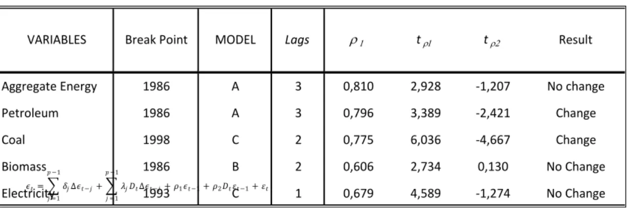
The results in Table 4 confirm the presence of very high levels of persistence for aggregate demand, petroleum products and coal and high but somewhat lower levels for biomass and electricity. In fact, the estimates of the levels of persistence presented here are not statistically different from the estimates presented in Table 1. More importantly from our standpoint, our results here suggest that we cannot reject the null hypothesis of a change in the level of persistence between the two sub-periods for coal and petroleum although we can do so for aggregate demand, biomass and electricity.
13
Table 4 - Testing changes in persistence: the parametric case
Aggregate Energy 1986 A 3 0,810 2,928 -1,207 No change
Petroleum 1986 A 3 0,796 3,389 -2,421 Change Coal 1998 C 2 0,775 6,036 -4,667 Change Biomass 1986 B 2 0,606 2,734 0,130 No Change Electricity 1993 C 1 0,679 4,589 -1,274 No Change MODEL Break Point
VARIABLES Lags r1 tr1 tr2 Result
𝜖𝑡= 𝛿𝑗∆𝜖𝑡−𝑗+ 𝜆𝑗𝐷𝑡∆𝜖𝑡−𝑗+ 𝜌1𝜖𝑡−1+ 𝜌2𝐷𝑡𝜀𝑡 −1 𝑝 −1 𝑗 =1 + 𝜀𝑡 𝑝 −1 𝑗 =1
5.2 The non-parametric cases
The test for changes in the level of persistence is based on the estimation of the following model [see Dias and Marques (2010)]:
𝑥𝑡 = 𝛼1+ 𝛼2𝑑𝑡+ 𝑢𝑡 (6)
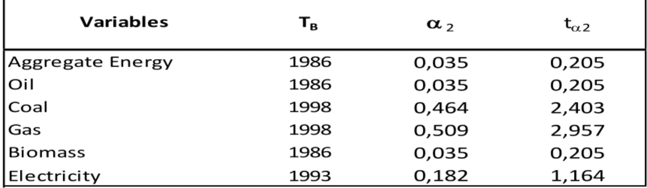
where 𝑥𝑡 is 1 if the series crosses its mean and zero otherwise and 𝑑𝑡 is a dummy variable that is 0 for 𝑡 ≤ 𝑇𝐵 and 1 otherwise. From (6), we can write that 𝛼1= 1 − 𝛾1 and 𝛼2= 𝛾1+ 𝛾2 where 𝛾1 and 𝛾2 are, respectively, the persistence measures for the first and second sub-period. Therefore, testing the change of persistence amounts to a test of whether 𝛼2 is significantly different from zero.
The results presented in Table 5 refering to the crash and growth case suggest we cannot reject at the 5% level of significance the null hypothesis of no change in the level of persistence for all fuel types excpet for coal and gas. For these two cases it would seem that the degree of persistence has declined after 1998. In turn, the results for the HP filter are reported in Table 6. In this case, the null hypothesis of no change in the level of persistence cannot be rejected in any case at the 5% level of significance. Electricity is a marginal case in that the null can be rejected albeit only at the 10% level indicating an increase in persistence after 1993.
14 Aggregate Energy 1986 0,035 0,205 Oil 1986 0,035 0,205 Coal 1998 0,464 2,403 Gas 1998 0,509 2,957 Biomass 1986 0,035 0,205 Electricity 1993 0,182 1,164 Variables TB a2 ta2
Table 6 - Testing changes in persistence: the HP Filter
Aggregate Energy 1986
0.035
0.172
0.205
Oil 19860.035
0.172
0.205
Coal 1998-0.009
0.253
-0.036
Gas 19980.109
0.160
0.680
Biomass 19860.035
0.172
0.205
Electricity 1993-0.253
0.174
-1.451
Variables TBa
2se
a2t
a2 5.3 The verdictOverall, our results fail to provide compelling evidence for changes in the levels of persistence between earlier and later sub-samples for the final demand for any of the fuel types under consideration. At the aggregate level, for biomass and electrictity the evidence is strongly in favor of no changes in persistence. There is some evidence in some of the tests for changes in the case of petroleum, coal, and gas. However, the results for coal and gas are not meaningful due to the small sample sizes for the second sub-period.
6. Summary and Concluding Remarks
Our results suggest for aggregate final energy demand in Portugal, consistently across different methodologies, the presence of a strong level of persistence and therefore a long memory of response to shocks. This is in contrast with, for example, the results for Turkey in Altinay and Karagol (2004) and for a panel of 182 countries in Narayan and Smyth (2007) where evidence for stationarity, understood as evidence for short-term memory responses, are reported. It is more in line with the time series results for Taiwan in Lee and Chang (2005) or with the results in Hsu, Lee, and Lee (2008), where it is shown that in only 13 of 84 countries is there evidence for stationarity and short-term memory. It is even more in line with the recent results in Lean
15
and Payne (2009) and Gil-Alana and Payne (2010) using fractional integration and therefore a more flexible framework for identifying the nature of memory of the response to shocks. Our approach allows also for a more flexible framework not only in terms of the measurement of persistence but also in terms of considering different types of fuel. In fact, using aggregate final energy demand as a point of reference, our results indicate that final demand for gas is the most persistent component of energy demand while the final demand for coal is the least persistent. In turn, final demand for petroleum and biomass tend to have levels of persistence similar to aggregate final demand. The case of final demand for electricity is inconclusive – it shows lower persistence than the average in the parametric tests, at the average in one of the non-parametric tests and above the average with the other.
These results have important implications for the design of environmental policies to reduce carbon dioxide emissions. The implications can be considered in absolute terms from an aggregate perspective or from the perspective of the demand of individual fuel types to highlight the ability to reduce energy consumption and thereby carbon dioxide emissions. The evidence for high persistent for aggregate demand as well as for petroleum, gas, biomass, and electricity, is good news. Strong persistence reflects strong habit formation mechanisms. Accordingly, programs for energy efficiency, subsidies for alternative energies or for that matter negative oil price shocks will tend to be more effective. Ultimately, environmental policies in Portugal can be implemented in a favorable setting in which their effects will tend to feed into themselves, be long lasting and larger.
The implications can also be considered from the perspective of the relative levels of persistence across different types of final energy demand and their implications for fuel switching. In a recent paper, Pereira and Pereira (2010) argue that for Portugal there are important opportunities from a macroeconomic perspective for fuel switching to reduce carbon dioxide emissions without hurting economic activity. In particular, the paper advocates policies that would shift final energy demand from low marginal abatement cost types of energy such as coal and petroleum to energy types such as gas and electricity which display high marginal abatement costs. Biomass, although limited by land and water requirements as well as conservation and biodiversity concerns, also represents a powerful avenue for satisfying final energy demand while substituting away from fossil fuels.
The question is how easy will be the implementation of these fuel switching opportunities in light of the differential levels of persistence in final energy demand we identify in this paper. In general, switching between types of energy with the same level of persistence is easier than
16
otherwise. In addition, switching to highly persistent types of energy is easier than for types of energy with lower levels of persistence. In our case, the high persistence of gas and the fact that biomass and petroleum have levels of persistence that are similar show by our persistence indicator fuel switching policies will be relatively easy to implement. The case of coal is somewhat different in that coal shows a great degree of inertia and switching away from coal may not be easy. This is not surprising since coal is nowadays a rather small fraction of aggregate final energy demand. In turn, the case of electricity, given our inconclusive results, is somewhat ambiguous. We know that electricity is also persistent and therefore shocks to its final demand will produce large and long lasting effects but we are not sure how these effects relate to the effects on the other final demand components.
References
Al-Iriani, M. (2006), “Energy-GDP relationship revisited: an example from GCC countries using panel causality,” Energy Policy 34, 3342-50.
Altinay, G. and E. Karagol (2004), “Structural breaks, unit root and the causality between energy consumption and GDP in Turkey,” Energy Economics 26, 985-94.
Chen, P. F. and C. C. Lee (2007), “Is energy per capita broken stationary? New evidence from regional based panels,” Energy Policy 35, 3526-40.
Cogley, T., G. E. Primiceri, and T. Sargent (2008), “Inflation-gap persistence in the U.S.” National Bureau of Economic Research Working Paper No. 13749.
Dias, D. and C. Marques (2010), “Using mean reversion as a measure of persistence,” Economic Modeling 27, 262-73
Direcção Geral de Energia e Geologia (2008), Balanços Energéticos. http://www.dgge.pt/ Elliot, G., T. Rothemberg and J. Stock (1996), “Efficient tests for an autoregressive root,”
Econometrica 64, 813-36.
Gadzinski, G., and F. Orlandi (2004), “Inflation persistence in the European Union, the Euro Area and the United States,” European Central Bank Working Paper No. 414.
Gil-Alana, L, J. Payne, and D. Loomis (2010), “Does energy consumption by the US electric sector exhibit long memory behavior?” Faculdad de Ciencias Economicas y Empresariales, Universidade de Navarra Working Paper 4/2010.
Hodrick, R. and E. Prescott (1981), “Post-war U.S. business cycles: an empirical investigation,”
Working Paper, Carnegie-Mellon. Reprinted in Journal of Money, Credit and Banking
29 (1) (1997), 1-16.
Hsu, Y. C., C. C. Lee, and C. C. Lee (2008), “Revisited: Are shocks to energy consumption permanent or temporary? New evidence from panel SURAFD approach,” Energy Economics 30, 2314-30.
Kwiatkowski, D., P. Phillips, P. Schmidt and Y. Shin (1992), “Testing the null hypothesis of stationarity against the alternative of a unit root,” Journal of Econometrics 54, 159-78.
17
Lean, H. and R. Smyth (2009), “Long memory in US disaggregated petroleum consumption: Evidence from univariate and multivariate LM tests for fractional integration,” Energy Policy 37, 3205-11.
Lee, C. C. (2005), “Energy consumption and GDP in developing countries: a cointegrated panel analysis,” Energy Economics 27, 415-27.
Lee, C. C. and Chang, C. P. (2005), “Structural breaks, energy consumption, and economic growth revisited: Evidence from Taiwan,” Energy Economics 27, 857-72.
Lee, C. C. and Chang, C. P. (2008), “Energy consumption and economic growth in Asian economies: a more comprehensive analysis using panel data,” Resource and Energy Economics 30, 50-65.
Levin, A. and J. Piger (2003), “Is inflation persistence intrinsic in industrial economies?” Federal Reserve Bank of St. Louis Working Paper No. 2003-023.
Marques, C. R. (2004), “Inflation Persistence: Facts or Artifacts?” European Central Bank Working Paper No. 8.
Mishra, V, S. Sharma, and R. Smyth (2009), “Are fluctuations in energy per capita transitory? Evidence from a panel of pacific island countries,” Energy Policy 37, 2318-26.
Narayan, P. K. and R. Smyth (2005), “Electricity consumption, employment and real income in Australia: evidence from multivariate granger causality,” Energy Policy 33, 1109-16. Narayan, P. K. and R. Smyth (2007), “Are shocks to energy consumption permanent or
temporary: evidence from 182 countries,” Energy Policy 35, 333-41
Pereira, A. and R. Pereira (2010), “Is fuel-switching a no-regrets environmental policy? VAR evidence on carbon dioxide emissions, energy consumption, and economic
performance in Portugal,” Energy Economics 32, 227-42.
Perron, P. (1989), “The great crash, the oil price shock and the unit root hypothesis,” Econometrica 57, 1361-401.
Pivetta, F. and R. Reis (2007), “The persistence of inflation in the United States,” Journal of Economic Dynamics and Control 31, 1326–58.
Willis, J.L. (2003), “Implications of structural changes in the U.S. economy for pricing behavior and inflation dynamics,” Economic Review - Federal Reserve Bank of Kansas City, First Quarter 2003, 5-27.
Zivot, E. and D. Andrews (1992), “Further evidence on the Great Crash, the oil-price shock and the unit-root hypothesis,” Journal of Business and Economic Statistics 10 (3), 251-70.