Entrepreneurship in Portugal : aggregate trend and evolution of the individual characteristics of entrepreneurs

(1)

Entrepreneurship in

Portugal: Aggregate Trend

and Evolution of the

Individual Characteristics

of Entrepreneurs

Paulo André Salvador

Dissertation written under the supervision of Hugo Reis

Dissertation submitted in partial fulfilment of requirements for the MSc in

Economics, at the Universidade Católica Portuguesa, Sep 7

th

_2018.

(2)

(3)

i

Entrepreneurship in Portugal: Aggregate Trend and Evolution of the

Individual Characteristics of Entrepreneurs

Paulo André de Mesquita Salvador Abstract

Entrepreneurship has a major role in economic growth, job creation and social mobility. However, it has been documented its decline in the past decade. We study entrepreneurship in Portugal between 1998-2014. We define entrepreneurs as self-employed with employees. The rate of entrepreneurship –that is, the proportion of entrepreneurs in the labor force– has decreased for the aggregate level and, also, for decompositions based on education level, area of residence and age group. We proceed to study the entrepreneurs’ characteristics such as age, education level, area of residence, gender and nationality. Entrepreneurs are older and more educated. We regress entrepreneurs on the previously mentioned characteristics. The highest coefficients are on older age groups and higher education levels, meaning that individuals with that particular set of characteristics are more likely to be an entrepreneur. Further, the Blinder-Oaxaca Decomposition is used to study the mean difference on being an entrepreneur; first, for the first and last year and, second, for every pair of consecutive years. We found that endowments have become more favorable to entrepreneurship. However, the coefficients effect dominates, decreasing the entrepreneurship mean. Thus, the coefficients on the characteristics have become lower. We study the most common previous occupational choices of entrepreneurs and find a surge of individuals leaving unemployment for entrepreneurship; yet the total entrance in entrepreneurship has decreased. Finally, we study the relation between aggregate entrepreneurship, real GDP growth and unemployment. However, we discard those two series as causes for the decline in entrepreneurship.

Resumo

O empreendedorismo tem um papel relevante no crescimento económico, na criação de emprego e na mobilidade social. Contudo, este tem vindo a diminuir na passada década. Estudamos empreendedorismo em Portugal entre 1998-2014. O empreendedor é definido como um trabalhador por conta própria que emprega. A taxa de empreendedorismo –proporção de empreendedores na população ativa– está diminuindo tanto em termos agregados como, também decompondo a mesma por grupos etários, níveis de educação e áreas de residência. Procedemos com o estudo das características dos empreendedores; como idade, género, nível de escolaridade, área de residência e nacionalidade. Os empreendedores estão mais velhos e têm maior escolaridade. Regredimos empreendedor nas características anteriores. Os coeficientes mais elevados são em grupos etários mais velhos e em indivíduos com maior escolaridade. Assim, indivíduos com estas características têm maior probabilidade de serem empreendedores. Em seguida, a Decomposição de Blinder-Oaxaca é utilizada para estudar a diferença na média de ser empreendedor; primeiramente, para o primeiro e último ano, seguidamente, para todos os pares de anos consecutivos. Descobrimos que a evolução das características é favorável ao empreendedorismo. Contudo, o efeito dos coeficientes é dominante, diminuindo a média de empreendedor. Assim, os coeficientes nas características diminuíram. Estudamos as anteriores ocupações dos empreendedores e descobrimos que há um aumento de anteriores desempregados que entram no empreendedorismo, contudo, a entrada total no empreendedorismo diminuiu. Por fim, estudamos a relação entre empreendedorismo agregado, crescimento real do PIB e desemprego. No entanto, excluímos estas séries como possíveis causas da diminuição do empreendedorismo.

(4)

(5)

ii

Acknowledgments

First and foremost, I would like to acknowledge to my closest family, my parents and my brother; also, to my two grandmothers and extended family. All of them had had a major role and contribution throughout my life and studies.

Further, I would like to acknowledge to my masters’ colleagues to whom I’ve spent a great deal of time studying and socializing and, also, to my thesis advisor, teachers that have lectured me and the Católica Staff.

While writing this thesis I had companions from my island that were also writing their thesis. We shared mutual motivation and support, to whom I shall thank.

(6)

(7)

iii

5.1.1. Age ... 13 5.1.2. Area of Residence ... 14 5.1.3. Education Level ... 15 5.2. ENTREPRENEURS’PROFILE ... 16 5.2.1. Age ... 17 5.2.2. Gender ... 18 5.2.3. Area of Residence ... 19 5.2.4. Education Level ... 20 5.2.5. Nationality ... 21 6. CONDITIONAL ANALYSIS ... 22 6.1. CHARACTERISTICS EFFECT ... 22 6.1.1. Methodology ... 22 6.1.2. Results ... 23

6.2. BLINDER-OAXACA DECOMPOSITION ... 26

6.2.1. Methodology ... 26

6.2.2. Analysis ... 29

7. ENTRANCE AND EXIT FROM ENTREPRENEURSHIP ... 34

8. ENTREPRENEURSHIP, GDP AND UNEMPLOYMENT ... 37

8.1. ENTREPRENEURSHIP AND GDPGROWTH ... 37

8.2. ENTREPRENEURSHIP AND UNEMPLOYMENT ... 39

9. CONCLUSIONS ... 41 9.1. LIMITATIONS ... 41 9.2. FUTURE RESEARCH ... 42 10. BIBLIOGRAPHY ... 43 A. APPENDIX ... 45 A.1.DATA ... 45

A.1.1. Variables Description ... 47

A.2.SECTION 5:ENTREPRENEURS ... 48

A.2.1. Decomposed Rates of Entrepreneurship ... 48

A.2.2. Entrepreneurs’ Profile ... 49

A.3.SECTION 6CONDITIONAL ANALYSIS ... 50

A.3.1. Linear Probability Model... 50

A.3.2. Blinder-Oaxaca Decomposition ... 51

A.4.SECTION 7:ENTRANCE AND EXIT FROM ENTREPRENEURSHIP ... 61

(8)

(9)

iv

Table Index

Table 1 - Labor Force Participation Rate ... 8

Table 2 – Number of Individuals by Occupational Choice and Percentages of the Labor Force ... 8

Table 3 - Age by Work Condition ... 17

Table 4 - Age Groups Proportions for the whole period ... 17

Table 5 - Gender ... 19

Table 6 - Area of Residence ... 19

Table 7 - Estimated coefficients of equation (1) ... 24

Table 8 - Correlation between GDP (percentage change) and Entrepreneurship Rate (percentage point change) – Correlation for figure 14 ... 38

Table 9 - Observations and Weighted Observations from 1998-2014 ... 45

Table 10 - Observations and Weighted Observations from 1998-2014 (continuation) ... 46

Table 11 - Entrepreneurship Rate Decomposed by Education Level ... 48

Table 12 - Entrepreneurship Rates Decomposed by Area of Residence ... 48

Table 13 - Entrepreneurship Rates Decomposed by Age Group ... 48

Table 14 - Age Group Proportions 1998 versus 2014... 49

Table 15 – Foreign Entreprenuers ... 49

Table 16 – Nationalities of the Entrepreneurs ... 50

Table 17 – Overall Oaxaca Decomposition Difference ... 54

Table 18 - Overall Oaxaca Decomposition Difference (continuation) ... 54

Table 19 – Oaxaca Decomposition Endowments Difference per year ... 55

Table 20 - Oaxaca Decomposition Endowments Difference per year (continuation) ... 56

Table 21 – Oaxaca Decomposition Coefficients Difference per year ... 57

Table 22 - Oaxaca Decomposition Coefficients Difference per year (continuation) ... 58

Table 23 - Oaxaca Decomposition Interaction Difference per year... 59

Table 24 - Oaxaca Decomposition Interaction Difference per year (continuation) ... 60

Table 25 - Outcomes of the Variables Condition Before Work and Work Situation ... 61

Table 26 - Condition Before Work Summary Statistics ... 62

Table 27 – Entrance and Exit from Entrepreneurship ... 62

Table 28 - Entrepreneurship, GDP and Unemployment rate from 1998-2014 ... 64

(10)

(11)

v

Figure Index

Figure 1 - Labor Force and Self-employment Evolution, in thousands ... 10

Figure 2- Self-Employment Rates Evolution ... 12

Figure 3 - Aggregate Entrepreneurship ... 12

Figure 4 - Entrepreneurship Rates by Age ... 13

Figure 5 - Differences between the average rates of 1998 and 2014 ... 13

Figure 6 - Entrepreneurship Rates by NUT ... 15

Figure 8 - Entrepreneurship Rates by Education Level ... 16

Figure 10 – Education Level of the Entrepreneurs ... 20

Figure 11 – Education Level of the Employees ... 20

Figure 12 - Oaxaca Decomposition: Decomposed Mean Difference of Entrepreneur, Year on Year 1998-2014 ... 31

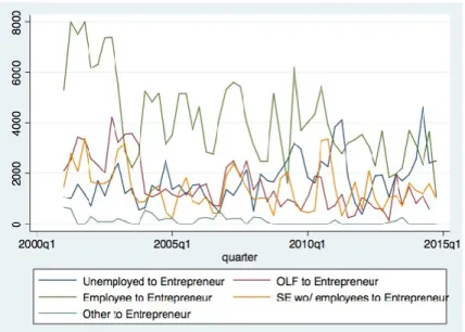
Figure 13 - Entrance into Entrepreneurship from Major Occupational Choices ... 35

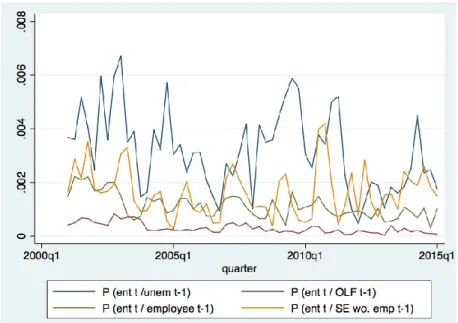
Figure 14 - Conditional Probability of Being an Entrepreneur at t Given the Occupational Choice at t-1 ... 36

Figure 15 - Real GDP Growth and Aggregate Entrepreneurship... 38

Figure 16 – Scatter of GDP growth to-year percentage change) and Entrepreneurship Rate (year-to-year percentage point change) ... 38

Figure 17 - Oaxaca Decomposition: Decomposed Mean Difference of Entrepreneur 1998 v 2014 .... 51

Figure 18 - Oaxaca Decomposition: Individual Contribution of the Endowments 1998 v 2014 ... 52

Figure 19 - Oaxaca Decomposition: Individual Contribution of the Coefficients 1998 v 2014 ... 52

Figure 20 - Oaxaca Decomposition: Individual Contribution of the Endowments Year on Year 1998-2014 ... 53

Figure 21 - Oaxaca Decomposition: Individual Contribution of the Coefficients Year on Year 1998-2014 ... 53

Figure 22 – Exit from Entrepreneurship to other occupational choices ... 62

Figure 23 - Entrance and Exit from Entrepreneurship ... 63

Figure 24 - Conditional Probability of Being an Entrepreneur at t Given that he/she was an Entrepreneur at t-1 ... 63

Figure 25 - Cross Correlogram First Difference of the Real GDP growth and First Difference of the Entrepreneurship rate ... 64

Figure 26 - Cross Correlogram First Difference of the Unemployment Rate and First Difference of the Entrepreneurship Rate ... 64

Figure 27 - Proportion of Firms by Type ... 65

Figure 28 - Proportion of GVA by Firm Type ... 65

(12)

(13)

Introduction

1

1. Introduction

Entrepreneurship is a driver of change. Entrepreneurial businesses introduce new goods, services and production processes that lead to a rise on living standards and generate long term economic growth (Smith, 1776; Schumpeter, 1942; Lucas, 1978). On a highly competitive fast pace world, the relevance and importance of these businesses for technological progress and competitiveness between countries is greater than ever.

The study of entrepreneurship is wide. Entrepreneurship has been linked to (1) economic growth, small and young businesses are associated with the creation of groundbreaking technologies and, these businesses also adapt faster and adopt more rapidly new technologies (Acemoglu et al. , 2013; Akipt and Kerr, 2015); (2) job creation, young and small firms are the greater net contributors to job creation in the US (Decker et al., 2014; Adelino et al., 2016); (3) economic mobility and inequality, opening a business might be a way to leave poverty and even become rich. In this topic the research differs once the mean income of an entrepreneur is usually lower when compared to a dependent worker (Quadrini, 2000; Canetti et al., 2006).

The study of entrepreneurship has recently become more relevant. It was documented that the aggregate rate of entrepreneurship (Hyatt and Spletzer, 2013; Decker et al., 2014; Kozeniauskas, 2017) –proportion of entrepreneurs in the labor force– has been decreasing for the US and, as we find, also in Portugal. The consequences of such decline in aggregate entrepreneurship are diverse, for instance: higher market concentration, higher income inequality, lower employment, and possible lower long-term economic growth. Thus, the study of entrepreneurship is complex and diverse. To study this reality, new and more complete datasets are becoming available opening the research for new contributions on this topic.

This dissertation aims to study entrepreneurship in Portugal. We start by studying aggregate entrepreneurship. For that we use data from the Portuguese Labor Survey from 1998 to 2014. The dataset that we use has some particular information, it divides the self-employed between self-employed with employees and self-employed without employees. The majority of the studies in entrepreneurship define an entrepreneur as a self-employed individual but we go further, defining an entrepreneur as a self-employed that employs. The aggregate rate of entrepreneurship is thus defined as the proportion of entrepreneurs, self-employed individuals

(14)

Introduction 2

that employ, in the labor force. We find that, as has been found for the US, aggregate entrepreneurship has decreased in Portugal by 1.4 p.p between 1998 and 2014. Further, we decompose the rate of entrepreneurship by age group, education level and area of residence. The first result holds for the majority of the decompositions, that is, the entrepreneurship rate has decreased in almost every region, for almost every age group and for almost all education levels. However, the decline is not homogeneous for all the decomposed subgroups.

Not everyone can become an entrepreneur. Individual characteristics play an important role. We study the role of individual characteristics as age, education level, gender, area of residence and nationality of the labor force participants in the likelihood of becoming an entrepreneur. First, we do it using the linear probability model for binary response for all observations, defining being an entrepreneur as the outcome variable and the characteristics of the individuals that belong to the labor force as the dependent variables. The coefficients on each characteristic represent how valuable such characteristic is, that is, having or not having a specific characteristic increases or decreases the probability of an individual to be an entrepreneur. Since the aggregate entrepreneurship rate has decreased we look for significant changes in the entrepreneur’s characteristics and labor force that might have justified such decrease. For that, in order to measure the changes in the coefficients and in the endowments, we use the Blinder-Oaxaca Decomposition, comparing the first year of our analysis, 1998, with the last year, 2014. Further, we do the procedure for every pair of consecutive years in order to analyze aggregate entrepreneurship during crisis and foreign economic aid and the subsequent recovery.

We found significant changes in the individual characteristics of the labor force in Portugal during these years. The labor force is older and more educated. These factors would, for a certain extent, increase the likelihood of an individual becoming an entrepreneur and, thus increase the aggregate rate of entrepreneurship. That is, the endowments effect in the Oaxaca Decomposition has actually played a positive role for entrepreneurship, since, at the end of our analysis, the labor force characteristics are more favorable to entrepreneurship. But the coefficients effect dominates the endowments effect in almost every year. The coefficients effect has the opposite sign of the endowments effect and is making aggregate entrepreneurship to decrease. Thus, the coefficients on the characteristics that we control for have become, on average, lower. Some other variables, exogenous, are the reason for such decline in aggregate

(15)

Introduction

3 entrepreneurship while, most of the individual characteristics –that we control for– are helping entrepreneurship, although, we do not assume causality.

The origin of the decline in entrepreneurship might be somewhere else besides the individual characteristics of the labor force. We complement our analysis by studying the previous occupation of the entrepreneurs and what they become after leaving entrepreneurship. Occupational backgrounds are related with individual skills, characteristics and preferences. The previous occupational choices studied are: being a salaried worker, being out of the labor force, being unemployed and being self-employed without employees. This study finds that while entrepreneurship has become more popular for the unemployed people, the entrance into entrepreneurship from all other occupational choices has declined. Adding to this, entrepreneurs maintain their position for longer periods of time, that is, if he/she already was an entrepreneur last year then it is more likely that he/she remains one. On the other hand, the former entrepreneurs leave entrepreneurship to become mostly employees or get retired.

Finally, we complement the temporal analysis of the entrepreneurship by studying macro data for that period. First, we analyze the relation between GDP and aggregate entrepreneurship, that is, to what extent changes in the aggregate entrepreneurship rate would affect changes in the gross product. Second, we study how unemployment and aggregate entrepreneurship relate; since both are mutually exclusive occupations, it would be expected that the relationship is negative. The relations between unemployment and GDP growth with aggregate entrepreneurship are studied in the literature. We find it interest to study the relations between those macro series with entrepreneurship because, in one hand, the results for Portugal may be different to the results for other countries, on the other hand, since we use a different definition of entrepreneurs, a stricter group of individuals, we might also reach different results.

The next section outlines the main studies in this area by topics. Section 3 does an overview of the data collected; section 4 defines an entrepreneur; section 5 characterizes the entrepreneurs; section 6 has the empirical analysis, presenting firstly the estimated results for the Linear Probability Model and, secondly, for the Oaxaca Decomposition while also introducing briefly these methods; section 7 evaluates the previous occupation backgrounds of entrepreneurs; section 8 relates aggregate entrepreneurship and unemployment with real GDP growth; section 9 concludes and comments on limitations and future research.

(16)

Literature review 4

2. Literature review

2.1. Declining entrepreneurship trend

The declining entrepreneurship trend has being documented in the United States by Decker et al. (2014) The authors of this study conceive entrepreneurship as a main driver of job creation and economic dynamism. Even tough, they refer the downward trend for entrepreneurial businesses in the US, they do not present reason for that so.

Then reasons for this decline in aggregate entrepreneurship are presented by Kozeniauskas (2017). This author uses a general equilibrium model of occupational choice that accommodates different reasons for the decline. The reasons studied for the decline in aggregate entrepreneurship are (1) skill biased technological change, (2) superstar firms hypothesis and (3) increases in the fixed costs either by changes in the regulation or technological change. Besides addressing this decline, this paper also shows that the decline has been higher for more educated individuals and that there has been a shift in the economic activity away from entrepreneurs. This study uses cross section micro level data on individuals to compute the aggregate rates of entrepreneurship, as this work that uses data on the labor survey. The main findings are that this decline is mainly due to increases in the fixed costs and skill biased technical change.

2.2. Demographics and entrepreneurship

In terms of demographics, entrepreneurs age is an important factor. There are different theories on this topic. On one hand, human capital tends to grow with age, certain skills need time and experience to be developed and young individuals lack them, skills as: decision making, leadership, market knowledge are intrinsically related with increasing with age and experience. This idea of need for on-job training is in line with the Becker’s model (Becker, 1964) on Human Capital. On the other hand, characteristics more common for younger individual are energy and creativity, as well as lower risk aversion.

(17)

Literature review

5 Liang et al. (2014) go far on this point and say that the age structure of the population has clear consequences on entrepreneurship. First, bigger older age cohorts are associated with higher competition in the labor market. These individuals are occupying the high-level management positions that are crucial to develop the skills needed to be a successful entrepreneur, postponing the younger cohorts’ development of these skills. The relation between entrepreneurship and age is then an inverted u-shape. Their results show that a decrease in the median age of the population increases the new business formation rate. Thus, it is expected that countries with a younger labor force experience greater rates of entrepreneurship, such as United States, compared to countries where aging process is quite intense, such as Japan. Adding to this, there is a rank-effect, that is, not only there are more entrepreneurs in younger countries, these countries also have higher rates of entrepreneurship for all age cohorts. On the other hand, age is also considered a key success predictor. Successful high growth firms are run by middle-aged people (Azoulay et al., 2018). The idea that young individuals are highly creative and capable of producing big ideas is not true. Instead, older founders are more likely to run successful firms.

2.3. Personality Traits of Entrepreneurs

Pekkala et al. (2017) do a review of recent studies on entrepreneurship in multiples areas. The main conclusion draw is that microeconmetric studies often do not include psychological variables or personality trait variables that might be important to predict entrepreneurship dynamics as well as highly successful outcomes.

Levine and Rubinstein (2015) have a very new approach studying this matter. First, they desegregate self-employment into incorporated and unincorporated. Second, they include variables such as exam scores, likelihood of doing illicit activities during studies and self-esteem levels on their analysis.

2.4. Entrepreneurship and Job Growth

Young firms are more responsive to changes. Although the lack of financing can be a constraint for this firms to seize new opportunities (Adelino et al., 2017). Once more, these firms’

(18)

Literature review 6

importance on job creation is referred, the role of their special characteristics, such as higher flexibility and higher innovativeness compared to non-entrepreneurial firms play an important role on their ability to generate jobs.

2.5. Modeling entrepreneurship

Modeling entrepreneurship is complex. Different models are used to study entrepreneurship. Occupational choice models are commonly used. Individuals chose between paid work, entrepreneurship and being out of the labor force based on their skills, preferences and on incentives of each occupational choice –that is, the wage rate of their type for each occupational choice. Lazear (2002) uses this type of model based on the hypothesis that entrepreneurs are not highly specialized but rather competent on very different skills and tasks. Also Kozeniauskas (2017) this type of model.

Regarding the entry, exit and firm dynamics Hopenhayn (1992) proposes a long run equilibrium proportion of business owners, i.e. entrepreneurs, in the labor force. Fixed costs and entry costs are found to have a great impact on firms’ earnings distribution and prevalence in the market.

In terms of the individual decision between paid work and self-employment, includes entrepreneurship, Dillon and Stanton (2017) model this using a life-cycle model of future earnings. Individuals will get to know better their prospective earnings as self-employed when they enter self-employment and they will keep learning about their earnings while they remain in self-employment. In case their future earnings are smaller for self-employment then they change back to paid work. This option of returning to paid work has high monetary value, individuals are more likely to experiment self-employment if they know for sure that they can easily get back to paid work. Adding to this, they evaluate policies for entering into self-employment by increasing incentives within the model’s framework. The two policies studied were, first, subsidies for entry into entrepreneurship and second, a flat tax rate for employment earnings. Both polices are effective in terms of increasing the entry into self-employment although neither policy has a net positive effect on Government’s Revenue.

(19)

Data

7

3. Data

We use data from the Portuguese Labor Survey from 1998 to 2014. The data is collected by the Portuguese Statistics Bureau (Instituto Nacional de Estatística). There are differences among the quarter observations. The Bureau has two different series for the period, one from 1998-2010 and another form 2011-2015. Within the same series some variables are extinguished, other added and some take different outcomes. Although, the variables used in this study are present in both series and are compatible by making some transformation in the case the outcome of a certain variables changes. Also, the survey follows individuals for six quarters. That makes it possible to evaluate the likelihood of an individual become an entrepreneur on a six-quarter period but not for the overall period. This particularity of using partial longitudinal information contained in the dataset is not exploited in this study.

To study entrepreneurship the dataset used is complete. It distinguishes between self-employed that do not have employees and self-employed that employ. That feature is not commonly found in datasets of this type neither used on the majority of the studies on entrepreneurship. The samples simple size is big. It consists of approximately 40 thousand observations for every quarter (Tables 9 and 10 – Appendix). Using frequency weights, we can get the approximate representativeness of each observation in the Portuguese population.

Nevertheless, the dataset has some limitations. Variables on personality or skills such as test scores, self-esteem levels, risk aversion, propensity to do small illegal activities, among others are not included in the dataset. These types of variables are of interest to study entrepreneurs either to study success of entrepreneurs, leading factors to enter entrepreneurship or just correlation, that is, which characteristics are more common among entrepreneurs. Also, it does not include data on income or wealth for the self-employed, making not possible to compute the returns to entrepreneurship. It also would be interesting to have more information related with the business ownership that the dataset does not contain. For instance, if the individual owns a business or not – not all self-employed necessarily own a business – and more data on the businesses owned: age, dimension, among others.

(20)

Data 8

3.1. Overview

It is important to know the dynamics of the population and of the labor force during 1998-2014. As Table 1 shows the population has increased by 1.8% increase, about 183 thousand individuals. The labor force also has increased by 1.5%. And, on the other hand, the Working Age Population has decreased, by 1.5% decrease, resulting on a higher Labor Force Participation Rate.

Table 1 - Labor Force Participation Rate

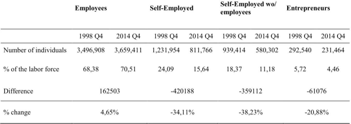
Table 2 – Number of Individuals by Occupational Choice and Percentages of the Labor Force

Employees Self-Employed Self-Employed wo/ _employees Entrepreneurs

1998 Q4 2014 Q4 1998 Q4 2014 Q4 1998 Q4 2014 Q4 1998 Q4 2014 Q4

Number of individuals 3,496,908 3,659,411 1,231,954 811,766 939,414 580,302 292,540 231,464

% of the labor force 68,38 70,51 24,09 15,64 18,37 11,18 5,72 4,46

Difference 162503 -420188 -359112 -61076

% change 4,65% -34,11% -38,23% -20,88%

Using the variable work situation (Table 25 – Appendix) to identify the entrepreneurs. This variable has 4 relevant different outcomes: the individual is an employee –that is, he or she works for someone else– the individual is self-employed without employees, the individual is self-employed and employs at least one employee and the individual is an unpaid family worker. Given the outcomes of the variable work type we can distinguish two types of self-employment: self-employed that does not employ and self-employed that employs. The sum of the two gives the total number of self-employed.

1998 2014 Population 10,184,997 10,368,054 Labor Force 5,113,733 5,189,857 Working age Population 6,872,417 6,769,649 Labor Force Participation Rate 74.41 76.66

(21)

Data

9

Self-employment has decreased both in total as well as decomposed into two subgroups. There are more inhabitants and more individuals in the labor force although self-employment has decreased while it would be expected to increase. Only the working age population has been reduced but that decline is considerably small compared with the decline on self-employment. Table 2 shows that the proportion of the Labor Force that were self-employed accounted for 24.09% of the Labor Force, in 1998, and only 15.64% in 2014. Self-employed without employees represented 18.37% in 1998 and by 2014, represent 11.18%. The self-employed with Employees accounted for 5.72% of the labor force in 1998 and, in 2014, 4.46%.

Self-employed has decreased more than a third. In 1998, 1,231,954 individuals were employed, in 2014, there is 811,766 individuals in this condition. There are less 420,188 self-employed in Portugal. The self-self-employed without employees has decreased by 38.2% while the employed with employees has decreased by 20.9%. The decrease on the total employed is mainly due to the employed without employees, 85% of the decrease in self-employment is from those individuals.

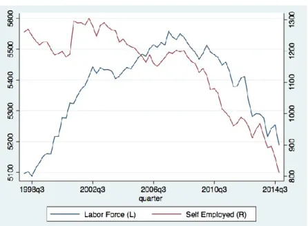
Regarding the dynamics over the period studied, Figure 1 shows that the labor force has increased until 2007, in that year it has reached the maximum of individuals. While the number of self-employed was already decreasing, it started decreasing approximately in 2001 or even earlier, and from that year on, the number of individuals with this occupation has been decreasing until at least late 2014. There is a flight of individuals from self-employment that antecedents the decrease on the labor force. In order to study entrepreneurship in more detail we strict our analysis to a subgroup of self-employment.

(22)

Definition of an entrepreneur

10

Figure 1 - Labor Force and Self-employment Evolution, in thousands

4. Definition of an entrepreneur

Defining entrepreneurship and an entrepreneur is difficult. Schumpeter’s definition of entrepreneurship is firms that can created highly innovative goods or production processes. The latter businesses will overtake the established ones, the process that was called “creative destruction”. Those firms are associated with the high-tech industry and produce great technological progress to the society. But that type of businesses is difficult to account. Because there is a lot of uncertainty on a firm’s success.

The most common definition of an entrepreneur in the literature is defining an entrepreneur as self-employed. Although, some of the self-employed might have liberal professions or be contracted workers such as housekeepers, lawyers, artists, architects, musicians, doctors, among others. They do not necessarily run and/or own a business. The dataset has that information but also has information on whether self-employed have employees.

Entrepreneurs are defined as Self-Employed that employ and this group is studied in more detail. This definition goes further than many other studies on entrepreneurship. Because it excludes self-employed that do not have any employee.

(23)

Definition of an entrepreneur

11 There is no guarantee that the defined entrepreneurs indeed run a business or are business owners, but it is highly expected that they do, once they have employees. Having employees is also a sign of commitment and responsibility. The definition used is a good proxy to study aggregate business ownership dynamics.

4.1. Aggregate Rate of Entrepreneurship

The aggregate entrepreneurship rate is the proportion of the labor force that are entrepreneurs. That is, self-employed with employees. The rate was computed for every quarter between 1998 to 2014.

To study the incidence of entrepreneurship for specific sub-groups, for instance different education levels, the following procedure is done:

𝑒𝑛𝑡𝑟𝑒𝑝𝑟𝑒𝑛𝑒𝑢𝑟𝑠ℎ𝑖𝑝 𝑟𝑎𝑡𝑒𝑖𝑡 =

𝑠𝑢𝑏𝑔𝑟𝑜𝑢𝑝 𝑜𝑓 𝑒𝑛𝑡𝑟𝑒𝑝𝑟𝑒𝑛𝑒𝑢𝑟_𝑖𝑡

𝑙𝑎𝑏𝑜𝑟 𝑓𝑜𝑟𝑐𝑒 𝑠𝑢𝑏𝑔𝑟𝑜𝑢𝑝𝑖𝑡

i denotes the different sub-groups, for instance age, educational level or area of residence

4.2. Alternative Definitions

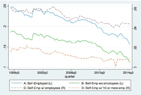
Alternative rates were also computed. Besides the entrepreneurship rate, the rates computed were: self-employment rate, rate for self-employed that do not have employees, rate for entrepreneurs, that have more than 10 employees. The denominator for all rates is the number of individuals in the labor force. The proportion of the labor force for all types of self-employment has declined.

(24)

Entrepreneurs 12

Figure 2- Self-Employment Rates Evolution

Figure 2 shows that independently of the definition used or the type of self-employment studied all has major declines. As stated in section 3.1., the self-employed without employees had the biggest decline. Even controlling for very small firms entrepreneurship, that is, excluding entrepreneurs with less than 10 co-worker, has decreased.

5. Entrepreneurs

There are less entrepreneurs in Portugal. There were 292.5 thousand entrepreneurs in 1998. In 2014, there were less 64 thousand entrepreneurs. The number of entrepreneurs has decreased by 20.88%.

(25)

Entrepreneurs

13 Aggregate entrepreneurship has declined from 5.9% to 4.5%. This decline might be different based for different groups of entrepreneurs. To evaluate that we decompose the aggregate rate of entrepreneurship by age groups, education levels and areas of residence to look for incidence of entrepreneurship among different groups.

5.1. Decomposed Rates of Entrepreneurship

5.1.1. Age

Regarding age, the rates of entrepreneurship were computed for 7 different age groups.

Figure 4 - Entrepreneurship Rates by Age

(26)

Entrepreneurs 14

The highest rates of entrepreneurship are for middle age individuals or older (Figures 4 and 5; Table 13 – Appendix). The age groups with the highest rates in 1998 were 50-59, 60-69 and 40-49 with 8.93%, 8.29% and 8.19%, respectively. For almost every age group the entrepreneurship rates have decreased. The rate for age group 50-59 had the biggest decline, decreased by 3%, followed by the age group 40-49, decreased by 2.7%. and by 30-39, decreased by 2.6%

On the other hand, entrepreneurship is becoming more common among the oldest age group, 70 or more years old had a major increase by 3%. The incidence of entrepreneurship among individuals in that age were not that big in 1998, but it has grown and has become the second age group with the highest incidence of entrepreneurship. One reason for high rates of entrepreneurship in this age group is that the majority of the employees are already retired. On the other hand, the very young have low rates

5.1.2. Area of Residence

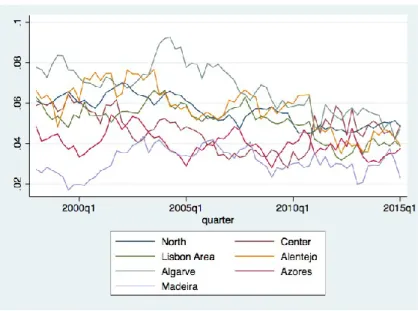
Algarve and Alentejo have the highest rate of entrepreneurship, with 7.7% and 6.6%, respectively, in the beginning of 1998 (Figures 6 and 7; Table 12 – Appendix). These two regions kept their leadership in terms of entrepreneurship rate on the majority of the period. On the other hand, Madeira and Azores have the lowest incidence of entrepreneurship, 2.7% and 4.8% in 1998, respectively. There are signs of a timid convergence the national average rates for those two regions.

Entrepreneurship has decreased in all regions of Portugal, excluding Madeira. The leading regions of entrepreneurship were the ones with biggest declines in percentage points, Algarve and Alentejo, 2.81 and 1.82 p.p. difference between 1998 and 2014, respectively.

(27)

Entrepreneurs

15

Figure 6 - Entrepreneurship Rates by NUT

Figure 7 - Differences between the average rates of 1998 and 2014

5.1.3. Education Level

Entrepreneurship is more common for individuals with lower levels of education (Figures 8 and 9; Table 11 – Appendix). Individuals with less than high school and individuals with high and some college. The ones that hold an undergrad degree had the highest rate in 1998, 6.23%, although it has decreased on the following years.

(28)

Entrepreneurs 16

Figure 8 - Entrepreneurship Rates by Education Level

Figure 9 - Differences between the average rates of 1998 and 2014

Entrepreneurship has decreased for all education levels. The higher levels of education were more affected as it was documented in the US by Kozeniauskas (2017). The least affected by the decrease were individuals that had less than high school.

5.2. Entrepreneurs’ Profile

The entrepreneur’s profile has changed during this period. Analyzing the entrepreneurs profile is complementary to analyzing the aggregate trend. What type of entrepreneurs are leaving entrepreneurship?

(29)

Entrepreneurs

17 This section compares the characteristics of entrepreneurs their evolution and compares them with the remaining occupational choices.

5.2.1. Age

Entrepreneurs are older than the employees but younger than the self-employed without employees. Entrepreneurs are, on average, 47 years old (Table 3). The mean of the entrepreneurs age is 7 years older than the overall population, 8 years older than the employees, and 7 years younger than the self-employed without employees.

Table 3 - Age by Work Condition

Population Employees Self-Employed Self-Employed wo Employees Entrepreneurs

Mean 40.4 38.8 51.9 53.7 46.9

Median 40 38 52 54 46

Std. Dev 22.73 11.56 14.62 15.08 11.68

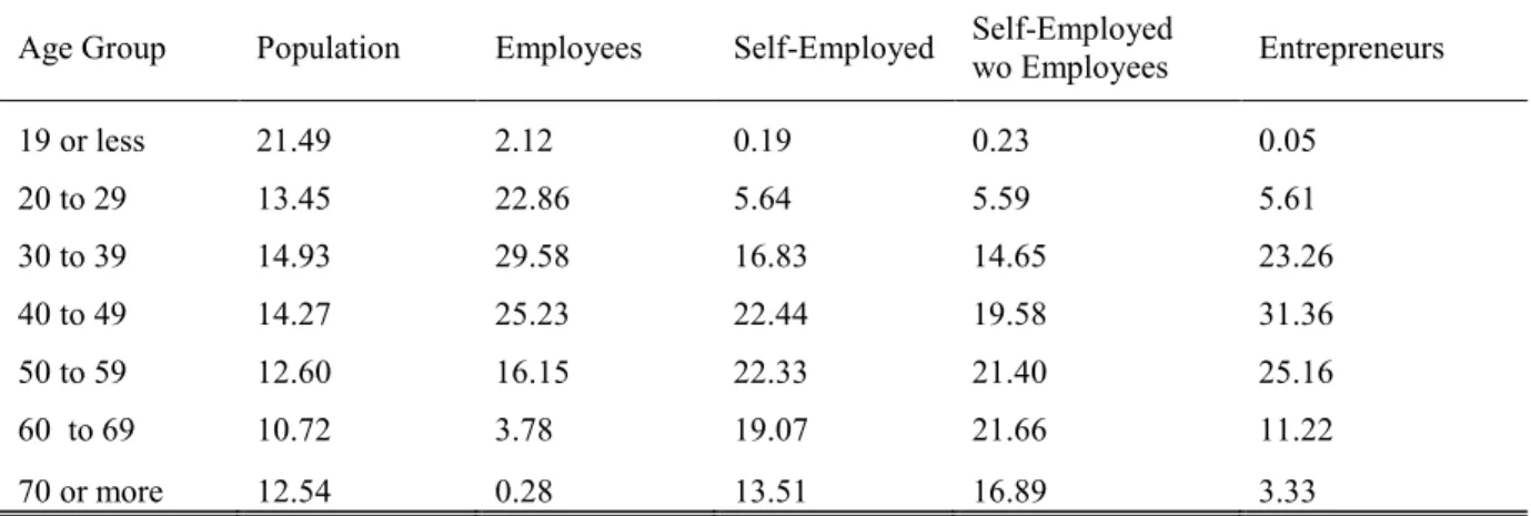
Table 4 - Age Groups Proportions for the whole period

Age Group Population Employees Self-Employed Self-Employed _{wo Employees} Entrepreneurs

19 or less 21.49 2.12 0.19 0.23 0.05 20 to 29 13.45 22.86 5.64 5.59 5.61 30 to 39 14.93 29.58 16.83 14.65 23.26 40 to 49 14.27 25.23 22.44 19.58 31.36 50 to 59 12.60 16.15 22.33 21.40 25.16 60 to 69 10.72 3.78 19.07 21.66 11.22 70 or more 12.54 0.28 13.51 16.89 3.33

Entrepreneurs are middle age or older (Table 4). Entrepreneurs with ages between 30 to 59 years old account for the majority of the entrepreneurs, 79.7% of the entrepreneurs are within this age group. Entrepreneurs younger than 30 are not that common, only 5.7%, and, on the other hand, entrepreneurs with 60 or more years old, are also not that common, account for 14.6%.

Employees are younger that entrepreneurs. There is a higher proportion of employees between 20 to 29, 22.9%, compared to the self-employed and lower proportions for older individuals,

(30)

Entrepreneurs 18

aged 60 or more, 4.0%. That is comprehensible to the extent that individuals enter the labor at between 20-29 and leave it at more than 60. Even though, the retirement age has changed during this period it never surpassed the 66 years old.

The later entrance in the entrepreneurship may have different reasons. Individuals need to acquire certain qualities and skills that take time and, more important, are learned working for someone else. On the other hand, certain skills decrease with age such has energy, risk aversion among others. Data shows that is unlike for very young people to open a business. Other reason besides skills that may justify the later entrance into entrepreneurship is based on the life cycle theory. Individuals need to save enough money to pay for the business fixed cost and entrance costs.

Entrepreneurs age follows the same pattern as the population and as the employees (Table 14 – Appendix). There are less very young entrepreneurs and more very old. The young entrepreneurs aged between 20 and 29 represent now only 2% while in 1998 they represented 8%. The proportion for the very old entrepreneurs has almost doubled, from 2.76% in 1998 to 4.18% in 2014.

The data suggests that the young which enter the labor force, aged between 20 and 29, are less likely to become entrepreneurs straight away. They are more likely to start as employees and then move to entrepreneurship. The proportion of individuals with that age is higher for employees that it is for all types of self-employment, and the proportion of middle age entrepreneurs is always higher. On the other hand, entrepreneurs are more likely to retire later than employees, the proportion of individuals with 60 or more is higher for all types of self-employment than it is for employees.

5.2.2. Gender

Table 5 shows that Woman surpassed men as employees. Women were less than men in 1994, 45.2%, while, by the end of 2014 they surpassed men on this group, accounting for 51.5%, this happened on the second quarter of 2010.

(31)

Entrepreneurs

19

Table 5 - Gender

Overall Employees Self-Employed Self-Employed _{wo Employees} Entrepreneurs

1994 2014 1994 2014 1994 2014 1994 2014 1994 2014 Male 48.22 47.36 54.77 48.46 58.94 65.03 54.03 62.31 74.72 71.83 Female 51.78 52.64 45.23 51.54 41.06 34.97 45.97 37.69 25.28 28.17

Woman’s participation into entrepreneurship registered a timid increase. Although participation of woman in entrepreneurship remains lower when compared to other occupational choices. Woman’s accounted for only 25.3% of the entrepreneurs, in 1998, and by 2014, they accounted for 28.2%.

5.2.3. Area of Residence

Table 6 show that the north of Portugal leads in entrepreneurship. It is the region in Portugal with more entrepreneurs. In 2016, almost half of the entrepreneurs in Portugal lived in the north and almost a third of the entrepreneurs in Portugal lives in the Lisbon area. Lisbon area and the north of Portugal have approximately the same number of inhabitants. Although, the north has considerably more entrepreneurs.

Table 6 - Area of Residence

Population Employees Entrepreneurs

1994 2014 1994 2014 1994 2014 North 35.63 35.01 36.18 34.53 37.92 40.29 Central 17.30 16.32 15.48 16.14 20.07 15.97 Lisbon 33.34 34.76 35.71 35.86 29.73 31.70 Alentejo 5.28 4.80 4.87 4.63 4.87 4.43 Algarve 3.71 4.22 3.37 4.02 4.87 3.99 Azores 2.36 2.39 1.88 2.29 1.50 1.85 Madeira 2.38 2.51 2.50 2.52 1.03 1.76

Central Portugal has had the biggest decline in entrepreneurship. The entrepreneurs living in central Portugal represented 20% of the total entrepreneurs in Portugal, in 1994. By the end of 2014 they represent less 4 percentage points.

(32)

Entrepreneurs 20

5.2.4. Education Level

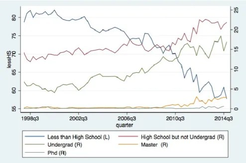
Portuguese entrepreneurs are becoming more educated. There are more entrepreneurs in all levels of education higher than having less than high school. Figure 10 shows that in 1998, entrepreneurs with the minimum level of education - having less than high school - accounted for more than two thirds of the total of the entrepreneurs. 16 years later the proportion of entrepreneurs with less than high school has decreased to just slightly more than a half.

Figure 10 – Education Level of the Entrepreneurs

(33)

Entrepreneurs

21

On the other hand, entrepreneurs with the very high level of education such as Masters or PhDs are unlikely. The proportion of entrepreneurs with masters starts to grow more significantly in 2009. Although, in 2014 is still lower than 5%. Entrepreneurs with PhD are rare. There is no clear sign of an increasing trend of entrepreneurs with PhDs.

The level of education in Portugal, during the time period studied, had major increases. There are less people with less than high school and increasingly more people with more than high school, undergrad degree, master’s degree and PhD. This upgrade on the level of instruction is higher and faster for the employees and for the entrepreneurs (Figure 10 and 11). By the end of 1998, almost 80% of the entrepreneurs had less than High School, by the end of 2014 they were 58%, for the employees 76% versus 46% by the end of 2014.

Comparing the education change of the entrepreneurs with the employees they look roughly similar. Entrepreneurs are not that more educated when compared to employees (Figure 11). Both groups have progressed, having more people with college degrees, but the proportion of employees with undergrad and master is higher than the one for entrepreneurs. By the end of 2014, 20.60% of the employees have an undergraduate degree versus 16.94% of the entrepreneurs and 4.22% of the employees had a master versus 2.83% of the entrepreneurs. In the contrary, there are very few entrepreneurs with very low education level, only 0.38% in 2014, has less than 3 years of schooling, while this proportion for employees is 1.11%.

5.2.5. Nationality

The vast majority of entrepreneurs in Portugal are nationals (Table 15- Appendix), only 1.63% of the entrepreneurs are foreigner in 1998. The proportion of foreign entrepreneurs has even decreased. There no dominant nationalities among the foreign entrepreneurs, that is, the majority of the most common nationalities of foreign entrepreneur in 1998 are no longer the same in 2014 (Table 16 – Appendix).

(34)

Conditional Analysis

22

6. Conditional Analysis

To help to characterize entrepreneurs and measure how do they differ from the remaining individuals in the labor force in terms of the studied characteristics. The study proceeds with the conditional analysis. Two methods are used to address the characterization. The linear regression model for all observation for all periods and the Oaxaca decomposition to measure the changes, on the effect and on the endowments.

6.1. Characteristics Effect

6.1.1. Methodology

To measure the effect of the entrepreneurs’ characteristics in the likelihood of one’s becoming an entrepreneur it used is a Linear Probability Model for Binary Response (LPM). In this model the coefficients estimated on the independent variables represent the increases or decreases in the probability of realizing the dependent variable.

The depend variable is equal to one if the individual is an entrepreneur and equal zero otherwise. The independent variables are age, educational level, gender, nationality and area of residence.

𝑒𝑛𝑡𝑟𝑒𝑝𝑟𝑒𝑛𝑒𝑢𝑟_𝑖 = 𝛽₁+ 𝛽_2𝑘𝑎𝑔𝑒𝑔𝑟𝑜𝑢𝑝_𝑘𝑖+ 𝛽_3𝑗𝑎𝑟𝑒𝑎 𝑜𝑓 𝑟𝑒𝑠𝑖𝑑𝑒𝑛𝑐𝑒_𝑗𝑖+

𝛽_4𝑙𝑒𝑑𝑢𝑐𝑎𝑡𝑖𝑜𝑛 𝑙𝑒𝑣𝑒𝑙_𝑙𝑖+ 𝛽₄𝑓𝑜𝑟𝑒𝑖𝑔𝑛 + 𝛽₅𝑓𝑒𝑚𝑎𝑙𝑒 + 𝜀_𝑖 (1) 𝑘 − 1, . . ,4 𝑗 − 1, . . ,6 𝑙 − 1, . . ,4

The coefficients are estimated by Ordinary Least Squares, standard errors and t test are robust. . The observations are weighted by a new generated variable that is the weights included in the dataset rounded, frequency weights. That way the observations reflect more closely the real proportions of the population.

The control variables included in the regression are the normal ones included on a wage regression. The literature assumes that these individual characteristics assume an important role for defining a worker’s productivity.

(35)

23 The base group of the regression is people who live in the North of Portugal, with age between 20 to 29 years old, with less than High School as education level, who are male and with Portuguese nationality.

Some concerns regarding the properties of the OLS estimators in a Linear Probability Model. Since the outcome variable y is a Bernoulli random variable –it only takes value 0 or 1– the variance of y is the probability of success P ( y=1 | x) times the probability of failure P (y=0 | x)=1- P (y=1 | x) (Equation A.2 – Appendix). The variance of the error term is equal to the variance of the outcome variable (Equation A.3 – Appendix). Thus, the variance of the error term depends on the regressors, making the errors heteroskedastic. A solution for heteroskedasticity in the Linear Probability Model is to use the White Robust Standard Errors and compute the t-ratios with this type of errors (Wooldridge, 2002).

The coefficient estimated by the linear probability model are unbiased and consistent (Equation A.1). However, this study is an empirical research and some concerns make the OLS estimators lose their properties. First, there is the possibility of omitted variables, there are definitely other variable that impact one’s likelihood of becoming an entrepreneur besides the ones we control for. This problem may overestimate or underestimate the coefficients of our model. Second, the control variables – independent variables - are all categorical, none is a continuous variable. The regressors are considerably restricted and that may turn the model a not so good description of the underlying response probability. However, the model is useful to characterize entrepreneurs and to study their changes, given the data used.

6.1.2. Results

It follows the estimated coefficients of equation (1), section 6.1.1. All regressions have a binary outcome, that is, the dependent variable is a dummy and is defined as one if the individual is an entrepreneur and zero otherwise, all the standard errors are robust.

(36)

24

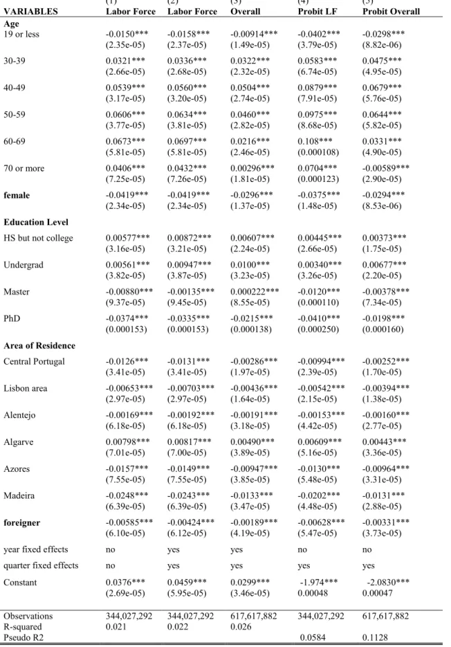
Table 7 - Estimated coefficients of equation (1)

(1) (2) (3) (4) (5)

VARIABLES Labor Force Labor Force Overall Probit LF Probit Overall Age

19 or less -0.0150*** -0.0158*** -0.00914*** -0.0402*** -0.0298***

(2.35e-05) (2.37e-05) (1.49e-05) (3.79e-05) (8.82e-06)

30-39 0.0321*** 0.0336*** 0.0322*** 0.0583*** 0.0475***

(2.66e-05) (2.68e-05) (2.32e-05) (6.74e-05) (4.95e-05)

40-49 0.0539*** 0.0560*** 0.0504*** 0.0879*** 0.0679***

(3.17e-05) (3.20e-05) (2.74e-05) (7.91e-05) (5.76e-05)

50-59 0.0606*** 0.0634*** 0.0460*** 0.0975*** 0.0644***

(3.77e-05) (3.81e-05) (2.82e-05) (8.68e-05) (5.82e-05)

60-69 0.0673*** 0.0697*** 0.0216*** 0.108*** 0.0331***

(5.81e-05) (5.81e-05) (2.46e-05) (0.000108) (4.90e-05)

70 or more 0.0406*** 0.0432*** 0.00296*** 0.0704*** -0.00589***

(7.25e-05) (7.26e-05) (1.81e-05) (0.000123) (2.90e-05)

female -0.0419*** -0.0419*** -0.0296*** -0.0375*** -0.0294***

(2.34e-05) (2.34e-05) (1.37e-05) (1.48e-05) (8.53e-06)

Education Level

HS but not college 0.00577*** 0.00872*** 0.00607*** 0.00445*** 0.00373***

(3.16e-05) (3.21e-05) (2.24e-05) (2.66e-05) (1.75e-05)

Undergrad 0.00561*** 0.00947*** 0.0100*** 0.00340*** 0.00677***

(3.82e-05) (3.87e-05) (3.23e-05) (3.26e-05) (2.20e-05)

Master -0.00880*** -0.00135*** 0.000222*** -0.0120*** -0.00378***

(9.37e-05) (9.45e-05) (8.55e-05) (0.000110) (7.34e-05)

PhD -0.0374*** -0.0335*** -0.0215*** -0.0410*** -0.0198***

(0.000153) (0.000153) (0.000138) (0.000250) (0.000160)

Area of Residence

Central Portugal -0.0126*** -0.0131*** -0.00286*** -0.00994*** -0.00252***

(3.41e-05) (3.41e-05) (1.97e-05) (2.39e-05) (1.70e-05)

Lisbon area -0.00653*** -0.00703*** -0.00436*** -0.00542*** -0.00394***

(2.97e-05) (2.97e-05) (1.64e-05) (2.15e-05) (1.38e-05)

Alentejo -0.00169*** -0.00192*** -0.00191*** -0.00153*** -0.00160***

(6.18e-05) (6.18e-05) (3.18e-05) (4.42e-05) (2.77e-05)

Algarve 0.00798*** 0.00817*** 0.00490*** 0.00609*** 0.00443***

(7.01e-05) (7.00e-05) (3.89e-05) (5.16e-05) (3.36e-05)

Azores -0.0157*** -0.0149*** -0.00947*** -0.0130*** -0.00964***

(7.55e-05) (7.55e-05) (3.85e-05) (5.48e-05) (3.31e-05)

Madeira -0.0248*** -0.0243*** -0.0133*** -0.0202*** -0.0131***

(6.39e-05) (6.39e-05) (3.47e-05) (4.48e-05) (2.88e-05)

foreigner -0.00585*** -0.00424*** -0.00189*** -0.00628*** -0.00331***

(6.10e-05) (6.12e-05) (4.19e-05) (5.47e-05) (3.73e-05)

year fixed effects no yes yes no no

quarter fixed effects no yes yes yes yes

Constant 0.0376*** 0.0459*** 0.0299*** -1.974*** -2.0830***

(2.69e-05) (5.95e-05) (3.46e-05) 0.00048 0.00047

Observations 344,027,292 344,027,292 617,617,882 344,027,292 617,617,882

R-squared 0.021 0.022 0.026

Pseudo R2 0.0584 0.1128

Robust standard errors in parentheses *** p<0.01, ** p<0.05, * p<0.1

(37)

25 Regression 2 (Table 7) is chosen because it controls for years and quarters, it restricts to individuals belonging to the labor force and are roughly similar to the Probit margins. The LPM model coefficients do not assume odd values; they represent the probabilities, and none is higher than 1 or lower than -1.

Setting all dummies equal to zero gives the constant of the regression. That is, one’s average probability with set of characteristics of the base group to be an entrepreneur. In this case, the probability for this group is 4.59% out of the labor force. Having or not having a specific characteristic increases or decreases the probability of a labor force individual to be an entrepreneur, compared to the base group. We do not assume causality, that is, a specific characteristic causes an individual to be an entrepreneur. The relationships between the independent variables (characteristics) and the outcome variable (being an entrepreneur) are of correlation.

The variable that has higher coefficients is age. For the all years’ regression, the age groups with higher coefficients are 50 to 59 years and 40 to 49. If the individual is between 50 and 59 years old the probability of being an entrepreneur increases by 0.0634 when compared to the base group. If the individual belongs to the age group that follows, between 60 and 69 years old, the probability increases by 0.0697 compared to the base group. A t-test was performed in order to access whether the coefficient on age group 60-69 is greater or equal than the coefficient on the age group 50-59. The p-value equals 0 thus we reject the null. Meaning that the age group between 60 and 69 is the likely among entrepreneurs.

Education level also has a significant role. Having high school and some college and holding and undergrad degree increases the probability of an individual being an entrepreneur. If an individual has high school and some college, the probability of being an entrepreneur increases by 0.00872 compared to the base group and by 0.0095 if he has an undergraduate degree. On the contrary, having a master’s degrees and a PhD actually decreases the probability of an individual to be an entrepreneur. The coefficients on different education levels suggest that, in one hand, entrepreneurs are, on average, more educated than the labor force and, on the other hand, individuals with very high levels of education such as PhD are unlikely to be entrepreneurs.

(38)

26

Regarding gender, female entrepreneurs are less, the probability decreases by 0.0419. As it was stated in section 5.2.2, there are significantly less entrepreneurial women both at the beginning and at the end of the analysis.

Only for an individual in Algarve is more likely to be an entrepreneur. The probability for the individuals that live in that region increases by 0.00817 compared to an individual that lives in the North. For every other region is less likely for an individual to be entrepreneur compared to the North of Portugal.

Lastly, foreign entrepreneurs are less likely than individuals with Portuguese nationality, if he or she is foreigner the probability of being an entrepreneur decreases by 0.00424 compared with the Portuguese.

The highest prevalence of entrepreneurship is among individuals that live in Algarve, with age between 60 and 69, that have High School or some college, that are Portuguese and male. Summing this all coefficients to the constant gives 0.1255 probability for this group.

On the other hand, the least likely incidence of entrepreneurship is among individuals that live in Madeira, that are 19 or younger, that hold a PhD, that are female and have foreign nationality. For this hypothetic group, the sum of the coefficients is negative and gives -9,61%. There is no individual that reunites those particular characteristics, just having a PhD with 19 or less years old is already rather impossible.

6.2. Blinder-Oaxaca Decomposition

6.2.1. Methodology

Once the effect of the independent variables is measured for the whole period considering all observations it is important to study how does this effect have changed along the period analyzed and measure the change on the mean value of the dependent variable. For that it is used the Blinder-Oaxaca Decomposition, this method determines differences in the mean of the dependent variables in two different groups as well as measures the contribution of each variable in the mean difference.

(39)

27 The decomposition was first introduced by Oaxaca (1973). This decomposition is frequently used for labor market outcomes such as to compute the gender gap, in this case, gender is the variable that splits the two groups. The coefficients are thus estimated for males and for females.

Weichselbaumer and Winter-Ebmer (2003) did a meta study of the predicted gender gaps, using Blinder-Oaxaca over time, for a variety of countries as well as draws some interesting advantages and disadvantages of this method. First, if the included characteristics are already affected by discrimination, this leads to underestimation of the group difference. Second, if the dependent variables are not good productivity predictors, or more precisely in this case, predictors of becoming an entrepreneur then the mean difference is biased upwards or downwards. Here, they refer to a twofold decomposition with an explained part and a unexplained part. The latter part is what is used as a discrimination indicator. If there is correlation between the omitted variables and the variable that separates the groups, often is gender, then the unexplained part might capture not only discrimination but also unobserved productivity differences between the two groups. We use years as the variable that splits the groups and so, the correlation between a year dummy and some omitted variables is possible. Using the threefold Oaxaca decomposition there is no need for a pooled model as it happens when using a twofold decomposition. The assumptions for pooled models are stronger, and in presence of unobserved heterogeneity the OLS estimates are inconsistent (Wooldridge, 2002). D denotes the difference in the mean outcome of the two group, unconditional on the regressors.

𝐷 = 𝐸(𝑌_𝐴) − 𝐸(𝑌𝐵)

Then we have a classical linear regression

𝑌_𝑖 = 𝑋′_𝑖β + 𝜀_𝑖

𝑋 is a matrix of regressors, it contains a constant, and 𝛽 is a vector of the coefficients, it contains the intercept.

(40)

28

The expected value of 𝑌𝑖 is equal to the expected value of the regressors times the coefficient

vector and the expected value of the error term equals 0, hence this difference D can be rewritten as

𝐷 = 𝐸(𝑋𝐴)′𝛽𝐴 − 𝐸(𝑋𝐵)′𝛽𝐵

To evaluate the contribution of the regressors in the mean difference. The difference D can then be decomposed into three parts (Jann, 2008):

𝐷 = [ 𝐸(𝑋_𝐴) − 𝐸(𝑋_𝐵)]′_𝛽

𝐵+ 𝐸(𝑋𝐵)′[𝛽𝐴 − 𝛽𝐵] + [ 𝐸(𝑋𝐴) − 𝐸(𝑋𝐵)]′[𝛽𝐴− 𝛽𝐵]

This decomposition is in the viewpoint of group B, once the differences in the endowments of A and B are weighted by the coefficient of group B and the differences in the coefficients are weighted by the predictors of group B.

Each part as a different meaning and can be interpreted as follows: 𝐴 = [ 𝐸(𝑋_𝐴) − 𝐸(𝑋_𝐵)]′_𝛽

𝐵

A reflects the part of the mean difference that is explained through the differences in the predictors, in this case, education level, age, gender, nationality and area of residence. This part is called the explained part of the difference because the model regressors are explaining this difference. It can be also interpreted as what would be the mean value of the outcome of group B if it had the same regressors as group A. This part is named the endowments effect. Then, we have

𝐵 = 𝐸(𝑋_𝐵)′_[𝛽

𝐴− 𝛽𝐵]

This part is the difference in the coefficients, is usually considered as the discrimination factor. The difference in the constants of the two groups is also included in here. This part is not explained by the dependent variables in the model it is rather fully unexplained, the effect of

(41)

29 this regressors on the depend variables changes across the two groups due to other exogenous reasons. And, finally:

𝐶 = [ 𝐸(𝑋_𝐴) − 𝐸(𝑋𝐵)]′[𝛽𝐴− 𝛽𝐵]

C is the interaction between the differences between the two groups in the coefficients and in the endowments. The part is partially explained and partially unexplained, the difference in the expected values of the regressors is explained, the difference in the coefficients is unexplained. The variable that defines the groups is a dummy that, first, equals zero if the year is 1998 and 1 if the year equals 2014, so the first and the last years analyzed. Then, we proceed analyzing year on year. For that we define dummies for each pair of following years, 1998-1999, 1999-2000, …, 2012-2013 and 2013-2014. In total were defined 17 dummies, one for the first and last year and 16 for each pair of following years between 1998 and 2014.

The regression was restricted by individuals belonging to the labor force in order to the mean value of the outcome variable, being an entrepreneur or not, be similar to the computed aggregate rate of entrepreneurship. We also control for quarter fixed effects.

6.2.2. Analysis

6.2.2.1. First and Last Year

The mean value of the dependent variable, the probability of being an entrepreneur, has decreased 0.014, or 23.7% (Table 17 – Appendix). The Blinder-Oaxaca method decomposes that difference into different parts, 3 in case is a threefold decomposition (previous section), and that give us information about the sources of this difference.

First, we have the endowments part, that is, if the characteristics of the labor force in 2014 were

the same as in 1998, it would be expected that entrepreneurship mean to increase1_{0.006 (Table}

17 and Figure 17– Appendix). Although this effect is outweighed by the second source of

1_{The difference due to endowments is negative and the mean of entrepreneurship has declined between 1998 and}

2014. The value of the mean difference is positive because is 1998 minus 2014. Hence, a negative value in the endowments part makes the mean to grow between 1998-2014.

(42)

30

difference: the coefficients. The differences in the coefficients accounts for the majority of the decrease in entrepreneurship 0.023. That is, the main source of the mean difference between groups is not explained by the dependent variables. Finally, the interaction part, a combination between the differences in the coefficients and the differences in the regressors, accounts for – 0.0028. It also contributes to a lower difference between groups.

The variables that contribute the most for the difference in the endowments are age groups and education levels. In detail, the differences in age groups 40-49 and 50-59, having an undergrad degree and in female are the main contributors (Figure 18 – Appendix). The population is older, more individuals hold an undergrad degree and there is more woman in the labor force in 2014 than in 1998. All of those facts worked in favor of a higher entrepreneurship incidence. The regressors in 2014 become more beneficial for entrepreneurship, but it is important to notice that strict exogeneity is not assumed, hence, there is no causality in the regressors. That is, there is no guarantee that the regressors are actual predictors of entrepreneurship.

As it would be expected, changes in the area of residence between the two groups were not that big and, thus, had almost no impact on the mean change between groups.

Regarding the coefficients’ changes, once more the effects of some age groups contributed the most for the mean difference (Table 21 and Figure 19– Appendix). On average, the coefficients of our model have decreased between 1998 and 2014. The coefficients represent the likelihood of an individual that possess or not specific characteristics and belongs to the labor force to be an entrepreneur. Once coefficients have decreased, the effect of the controlled characteristics on being an entrepreneur has become lower. The coefficients on the age groups 30-39, 40-49 and 50-59 had major declines, as well as the coefficient on HS and some college. In the contrary, the coefficient on female had a major increase.

The first and last year analysis is limited. The decline on the mean of entrepreneurship for the labor force between 1998 and 2014 may be caused by specific year effects or different business cycle faces. Thus, it is necessary to evaluate the changes year on year.

(43)

31 6.2.2.2. Year on Year

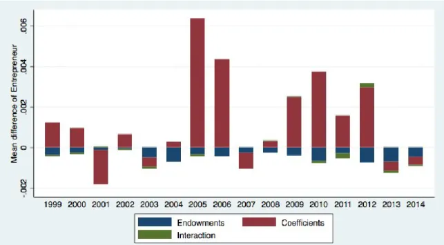
In the majority of the period, aggregate entrepreneurship decreases. Figure 12 shows the difference in the mean of the outcome variable: being an entrepreneur. At each year the mean difference results from the mean for the previous year minus the mean for that year. That is, if the mean difference is positive, then aggregate entrepreneurship has decreased in that year compared to previous year, and, if it is negative, then aggregate entrepreneurship has increased.

Figure 12 - Oaxaca Decomposition: Decomposed Mean Difference of Entrepreneur, Year on Year 1998-2014

Note: Endowments, Coefficients and Interactions results were computed using the threefold Blinder-Oaxaca

Decomposition. The sum of endowments, coefficients and interaction equals the difference in the outcome variables, being an entrepreneur. The values for each year result from the difference between that year and the previous year. Thus, if sum of the endowments, coefficients and interaction is greater than zero then aggregate entrepreneurship decreases and if the sum of the three is negative then aggregate entrepreneurship increases.

The biggest decline in aggregate entrepreneurship is in 2005 and 2006, as shown is Figure 12. In 2005, real GDP has increased by 0.8% in 2005 and by 1.6% in 2006. Thus, in this period both series have changed in different direction and with different magnitudes. Suggesting that the relation between real GDP and the aggregate entrepreneurship is quite limited.

The second biggest decline happens in 2009 and 2010, comparing to the previous year. These were the years that followed the financial crisis. Between beginning of 2008 and 2009 Portugal has negative growth rates of real GDP. Suggesting this financial crisis has some impact on aggregate entrepreneurship. On one hand, the crisis affected heavily the banks. Major banks in