1
Contagion effects of the US Subprime Crisis on Developed
Countries
Paulo Horta,Comissão do Mercado de Valores Mobiliários
Carlos Mendes, UNINOVA – DEE and FCT, Universidade Nova de Lisboa
Isabel Vieira, CEFAGE–UÉ and Departamento de Economia, Universidade de Évora
Introduction
The burst of the US mortgage bubble, in early August 2007, was an abrupt waking up call for financial markets worldwide. Until then, even though interventions by central banks suggested the possibility of a more serious impact, the effects of the subprime crisis were mostly confined to the US. The first significant liquidity injection by the European Central Bank took place on 9 August and was followed by similar actions by other major central banks. By supplying low cost money, monetary authorities wanted to ensure that commercial banks could maintain a normal level of activity despite the increasing difficulties faced in the interbank money market. At the time, banks almost stopped mutual lending, either anticipating future losses, and thus the need to build up adequate levels of reserves, or simply reacting cautiously to the turmoil in the financial system and to the uncertainties concerning the real dimension of the crisis.
The most severe and widespread effects were not yet visible in the autumn of 2007, but were already anticipated. On the 15 of October, the president of the Federal
2
Reserve referred that the developments of the relatively small US subprime market were having a large impact upon the global financial system. In fact, losses associated with the subprime crisis were being reported by financial institutions all over the world, namely in the G7 countries. Examples were the Citigroup in the US, the Crédit Agricole in France, HSBC in the United Kingdom, CIBC in Canada, or the Deutsche Bank in Germany.
These episodes suggested that the burst of the US mortgage bubble was affecting other markets, in a contagious process similar to what occurred in previous crises. In the past, evidence of financial contagion emerged in empirical assessments, mostly focused on the dependence structure of stock market indices in turbulent periods (see, for
instance, Bae et al., 2003). Specifically, Cappiello et al. (2005) showed that the financial crises occurred in the 1990s in Asia and Russia affected Latin American markets, and Rodriguez (2007) found evidence of contagion in both the Asian and the Mexican crises. In this study, we check whether contagion was also visible in the case of the subprime crisis. The reported distress signs suggested that this could have been the case from an early stage and we analyse the behaviour of the G7 countries’ stock market indices in the seven months that followed the burst of the mortgage bubble to formally assess such hypothesis.
To this end, we study a time sample covering a period that precedes August 2007 (the pre-crisis period) and the first months that followed (the crisis period), using the copula methodology and adopting the concept of contagion proposed by Forbes and Rigobon (2001). From their perspective, financial contagion is ‘a significant increase in cross market linkages after a shock to one country (or group of countries)’.i
3
zero market) and the other markets in the sample, from the pre-crisis to the crisis period, may be interpreted as evidence of contagion. Although the focus of our attention is the G7 markets, Portugal is also included in the study, in an attempt to evaluate contagion effects in more peripheral areas.
The remainder of the study is organised as follows: section two briefly surveys the relevant aspects of the copula theory; section three presents the data and justifies the adopted methodology; section four displays the empirical analysis and respective results; section five concludes.
Copula theory
The adoption of the copula methodology is still relatively new in the financial context but copulas have already been used in various studies, namely in contagion
assessments.ii The concept was introduced by Sklar (1959) and may be used as an
alternative to correlation coefficients, or to other measures of relationships between variables requiring strong conditions rarely met by financial data.
A copula is a joint distribution function of random variables, with pre specified
properties (see, for instance, Schmidt, 2006). According to Sklar (1959), it is possible to split the joint distribution into two basic components: the marginal variables, following a uniform distribution in the interval [0, 1], and a function of dependence between such variables (the copula).iii One important tool in this rationale is a fundamental result from
the Fisher’s theory of random numbers (Fisher, 1932), which states that if X is a random continuous variable with a distribution function F , then U =F
( )
X follows a uniform distribution between 0 and 1, regardless of the shape assumed by F . The variable U is4
known as the probability integral transformation of X. A copula is thus a function
expressing the links amongst univariate distribution functions in a joint distribution. It is precisely this characteristic that inspired Sklar in designating such function as a copula, a word of Latin origin that means connection or junction (Patton, 2002).
Formally, the Sklar theorem states that any d dimensional function F , with univariate marginal functionsF ,...,1 Fd, may be written as:
(
x xd)
C(
F( )
x Fd( )
xd)
F 1,..., = 1 1 ,..., , where C represents the copula.
If X =
(
X1,...,Xd)
is a vector of random variables, the copula function is givenbyC
(
u ud)
F(
F( )
u Fd( )
ud)
1 1 1 1 1,..., ,..., − −= , where Fi−1 represents the inverse marginal
distribution function i , with Ui ~ Unif
( )
0,1 (Nelsen, 2006).Deriving both sides of the first equation in order to each marginal variable, to obtain the density functions (here represented in lower case letters), the copula’s role as a dependence structure is clear:
(
)
(
( )
( )
)
( )
( )
( )
( )
d d d d d d d d d d d x x F x x F x F x F x F x F C x x x x F ∂ ∂ × × ∂ ∂ × ∂ ∂ ∂ = ∂ ∂ ∂ ... ... ,..., ... ,..., 1 1 1 1 1 1 1 1 1 or(
x xd) (
cu ud) ( )
f x fd( )
xd f 1,..., = 1,..., × 1 1 ×...×The above equation shows that, when the copula is neutral, the joint function is equal to the product of the marginals. In this case, all variables in vectorX =
(
X1,...,Xd)
are independent. If the copula density function is not neutral, it represents a dependence link amongst the variables in X.
One advantage of the Sklar’s theorem is its flexibility in multidimensional modelling. For instance, knowing the marginal distribution functions (which do not
5
have to be identical) and knowing the copula function (that may be chosen independently from the marginal distributions), the joint distribution function is obtained by direct application of the theorem.
In this study, the main objective is to analyse the dependence structure between pairs of stock indices. This may be achieved by selecting the adequate univariate distribution functions for the marginals and the appropriate copula to link them, and then using the information obtained with the probability integral transformation of the marginals in the process of copula estimation.
The Gaussian approach, often adopted in similar contexts may be discarded as it could be inappropriate in this context for not being able to capture the asymmetric dependence frequently present in bidimensional series. Longin and Solnik (2001), Ang and Chen (2002), and Ang and Bakaert (2002), for instance, suggested that financial assets’ returns appear to be more correlated in bearish than in bullish markets. In view of such asymmetry, approaches that rely on normality assumptions should not be adopted. The copula approach is thus more reliable as it may be used regardless of the specificities of the series’ distributions.
A variety of copulas has been proposed (see for instance Nelsen, 2006), but in finance the most commonly adopted are the Gaussian copula (Lee, 1983), the t Student copula and some Archimedean copulas, such as the Gumbel copula (Gumbel, 1960), the Clayton copula (Clayton, 1978) or the Frank copula (Frank, 1979). When the variables present symmetric dependence structures, Gaussian or t Student copulas may be adopted. If the dependence is more visible in the left of the distribution, the Clayton copula is more adequate. The Gumbel copula should be used in cases of right hand side dependence (Trivedi and Zimmer, 2005).
6
The Gumbel and Clayton copulas cannot be used to model negative dependence structures, but this should not be a problem for data on stock indices, since dependence between them is usually positive. The Frank copula is symmetric but has some
advantages in relation to the Gaussian and the t Student copulas, namely to allow a more straightforward estimation of the dependence parameter, due to its simple analytical form. This copula is also appropriate to model variables displaying bands with weak dependence structures (Trivedi and Zimmer, 2005).
As an example, the functional forms of the Clayton and Gumbel copulas are displayed:
(
)
θ
θ
θ
1 1 2 1 2 , 1 − − + − − = u u u u Clayton C ,where
θ
∈(
0,+∞)
represents the parameter of dependence between the marginalvariables, 1
( )
1 1 1 F U X = − and 1( )
2 2 2 F UX = − , being F1 and F2 the distribution
functions of X1 andX2, respectively. Values of
θ
approaching zero, represent independence between the two variables. Larger values portray higher levels of dependence.The Gumbel copula is represented by:
(
)
(
) (
)
− + − − =θ
θ
θ
1 2 ln 1 ln exp 2 , 1 u u u u Gumbel C ,where the dependence parameter is
θ
∈[
1,+∞)
. Ifθ
=1, variables X1 and X2 are independent. As before, the larger the value ofθ
, the stronger the dependence between variables. Figure 1 displays simulations of the Clayton and Gumbel copulas for distinct dependence parameters.7
Figure 1. Simulations of Clayton and Gumbel copulasiv
The Clayton copula, in panel 2, displays a more centred distribution than that of panel 1, thus exhibiting a higher level of dependence. Furthermore, the left hand side of the Clayton copula is tighter than its right hand side, where the points are more
scattered. Such patterns could thus represent market indices exhibiting stronger trends in down markets.
If the copula in panel 1 portrayed the dependence structure between two markets in a period of calm, and that in panel 2 represented the same markets’ dependence in a period of crisis, the two would convey evidence of financial contagion.
In addition to ‘pure’ copulas, mixed ones may also be used (see, for instance Dias, 2004). The combination of a Gumbel and a Clayton copula, for instance, has the advantage of being adequate in the analysis of almost perfect symmetry and also for asymmetric cases.
8
(
u1,u2)
w1CClayton(
u1,u2)
w2CGumbel(
u1,u2)
mix
C = + ,
where w1,w2∈
[ ]
0,1 and w1+w2 =1.As w1 tends to one, the mixed copula approximates the Clayton copula, reflecting a more pronounced dependence in the left hand side of the mixed copula. Conversely, when w1 tends to zero, the right hand side of the mixed copula is more prominent. The mixed copula may also capture independence between variables, a scenario that would produce values close to zero and to one for the Clayton and the Gumbel copulas’ dependence parameters, respectively.
Data and methodology
In this study, the copula methodology is adopted to formally compare dependence relationships between stock indices in the period of relative financial stability preceding the sub-prime crisis, here designated as the pre-crisis period, and in the first months of the turbulent phase that followed. The sample of data for the pre-crisis period begins on 1 January 2005 and ends immediately before the burst of the mortgage bubble, assumed to have occurred on 1 August 2007. The crisis period starts at the beginning of August and extends until 29 February 2008, the last day for which data on stock market indices were collected. Daily closing values for the Morgan Stanley Capital International (MSCI) indices, in local currencies, are used for the G7 and the Portuguese markets. With such data, series of daily returns are constructed.
The objective is to analyse the structure of dependence between the US stock market and each of the other markets, in the pre-crisis and in the crisis periods. The
9
following pairs are thus assessed: Germany, Canada, France, Italy, US-Japan, US-Portugal and US-UK. The bivariate series are slightly distinct in length to calibrate the pairs of data according to each country’s national holidays.v
As previously noted, the Pearson’s linear correlation coefficient could also be used to quantify dependence. However, authors such as Boyer et al. (1999) or Forbes and Rigobon (2001) have shown that it may produce weak results when the variables exhibit conditional heteroskedasticity or autocorrelation. According to Corsetti et al. (2005), if the variables are not independent and identically distributed (iid), the
corrections to accommodate the instability of the distributions’ mean and variance may still produce biased results. Furthermore, Embrechts et al. (2003) and McNeil et al. (2005) suggest that the correlation coefficient is robust as a measure of dependence only in the case of elliptic distributions, an example of which is the Gaussian distribution, and alternatives should thus be thought when this is not the case. Following such
potential problems, we follow Costinot et al. (2000) who suggested the use of copulas, a tool that allows both an integral characterisation of dependence between variables and a quantitative assessment of hypotheses on such links, for instance recurring to scalar synthetic measures of rank correlation such as the Kendall’s
τ
or the Spearman’sρ(Schmidt, 2006).
Rank correlations are very useful tools in this context because dependence coefficients from distinct types of copulas may be non-comparable. Recall that, as shown above, their intervals of variation may be distinct.vi
Rank correlations, on the other hand, are always comparable as they are comprised between -1 and 1, and are invariant to non linear transformations of the variables, as long as they are monotonic,
10
which is the case for probability integral transformations performed on the marginal variables.
In this analysis of financial contagion, the Kendall’s
τ
and the Spearman’sρare used as synthetic measures of dependence between the US and the other markets’ indices. These parameters are directly obtained from each copula’s function (Nelsen, 2006):
(
)
= 1∫ ∫(
(
)
−)
0 2 1 1 0 2 1 2 , 1 12 2 , 1 X C u u u u du du X Spearmanρ
(
)
∫ ∫(
) (
)
∂ ∂ ∂ ∂ − = 1 0 2 1 1 0 2 2 , 1 1 2 , 1 4 1 2 , 1 du du u u u C u u u C X X Kendallτ
.In order to be able to formally test contagion, the following four-step methodological procedure is adopted:
Step 1: The series’ autoregressive and conditional heteroskedastic effects are removed with ARMA-GARCH models and the resulting residuals, denominated filtered returns, are assessed for mean and variance stability.
Step 2: The series of filtered returns are divided into two periods (the pre-crisis and the crisis period) and a number of distribution functions are estimated by maximum likelihood for each series (Gaussian, t location-scale, logistic, Gumbel and extreme value distributions). The Akaike information criterion (AIC) is used to select the most adequate distribution for each case.
Step 3: The selected distributions are utilised in the maximum likelihood estimation of various pure and mixed copulas (the Clayton, Gumbel, Frank, Gaussian, t Student, Clayton-Gumbel, Gumbel-Survival Gumbel and Clayton-Gumbel-Frank copulas), and the AIC is again employed to select the most appropriate. This method of
11
estimating the copulas is designated by McLeish and Small (1988) as Inference Functions for Margins (IFM) and consists of firstly estimating the marginal
distributions’ parameters and then using them in the process of estimating the copulas. One main advantage of such procedure is the possibility of testing the goodness of fit of the marginal distributions before estimating the copulas.
Step 4: The bootstrap technique proposed by Trivedi and Zimmer (2005) is used to calculate the variance-covariance matrix for the selected copulas’ estimated
parameters (matrix V ).
This bootstrapping procedure consists of adopting the IFM method to estimate
the vector of marginal distributions’ parameters,
∧
1
β
and∧
2
β
, and the vector of the copulas’ parameters,∧
θ. The vector of all estimated parameters is ( 1, 2, )T
∧ ∧ ∧ = ∧ Ω
β
β
θ
. A sample of ‘observations’ obtained from the original data is then constructed in a random draw with reposition. This sample is used to re-estimateβ
1,β
2 andθ
with the IFM method. The second and third procedures are replicated R times, with the rthre-estimation identified by Ωˆ
( )
r =(
β
ˆ1( ) ( ) ( )
r ,β
ˆ2 r ,θ
ˆ r)
T . The parameters’ standarddeviations are the square roots of the main diagonal elements in matrix V , estimated as
∑ = ∧ Ω − ∧ Ω ∧ Ω − ∧ Ω − = ∧ R r T r r R V 1 ) ) ( )( ) ( ( 1 .
The output of the bootstrap results, namely the Kendall’s
τ
and the Spearman’sρ, are used to develop two tests of financial contagion. The first assesses whether dependence between the US and each of the other countries increased from the pre-crisis to the pre-crisis period. This test’s null hypothesis is the absence of contagion:
12 > − − = ∆ ≤ − − = ∆ 0 : 1 0 : 0 crisis pre crisis H crisis pre crisis H τ τ τ τ τ τ or > − − = ∆ ≤ − − = ∆ 0 : 1 0 : 0 crisis pre crisis H crisis pre crisis H ρ ρ ρ ρ ρ ρ
The second test checks the hypothesis of distinct contagion intensity across markets. If contagion was more intense in market A than in market B, the increase in dependence between the US market and market A, from the pre-crisis to the crisis period, is stronger than that between the US market and market B. The null hypothesis in this case is one of homogeneous contagion intensity:
> − − − − − = − ∆ ≤ − − − − − = − ∆ 0 : 1 0 : 0 B crisis pre B crisis A crisis pre A crisis B A H B crisis pre B crisis A crisis pre A crisis B A H
τ
τ
τ
τ
τ
τ
τ
τ
τ
τ
Estimation and testing results
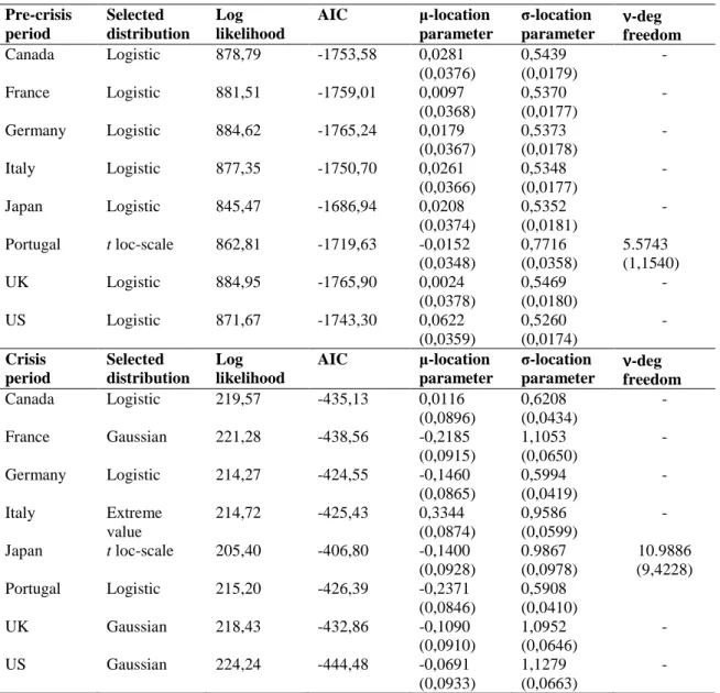
In the sake of brevity, the specific details involved in each of the four steps described above are presented in Annexes A and B. The procedures that lead to the series of filtered returns are described in Annex A. Various distribution functions were then estimated by maximum likelihood. Information on the distinct functions is available in table 1.B, in Annex B. Taking into account the AIC, the logistic distribution appears to be the best alternative. The shape of this distribution is similar to that of the t Student, thus suggesting the existence of heavy tails in the series of filtered returns. Only the
13
Italian market displays some asymmetry, during the crisis period. All remaining cases appear to be symmetric.
Estimating copulas for the bivariate series, in the pre-crisis and the crisis periods, is the following step. Tables 2.B and 3.B, in Annex B, display the various estimates for all markets, in the two periods. A number of aspects are of interest:
- Firstly, the various estimated copulas’ parameters increase in value from the pre-crisis to the crisis period, thus suggesting that the co movements between markets became more pronounced after the burst of the mortgage bubble.
- Secondly, the level of dependence between each of the markets and the US, before the crisis, is non-homogeneous. Focusing on the results for the t Student copula, only, the Canadian market displays the highest level of dependence, with a coefficient of 0,6262. The German, French, Italian and UK markets exhibit lower levels of dependence, presenting values around 0,45. The least dependent markets are the Japanese (0,3761) and the Portuguese (0,2192). In spite of the distinct levels presented by the dependence coefficients, they are all positive, thus suggesting that each market was already positively connected with the US before the crisis.
- Finally, the t Student copula appears to be the most adequate to model dependence between the markets in the pre-crisis period, whereas the Frank copula outperforms the others for the crisis period. In this latter period, the copulas selected by the AIC present a symmetric structure. The only exception is the Japanese market whose connection with the US is represented by the Gumbel copula. These results contrast with previous work suggesting that markets appear to be more connected in down markets.
14
Table 4.B, in Annex B, contains relevant information on the selected copulas: estimates for the copulas’ parameters,
θ
, and for the rank correlation coefficients,τ
and ρ. Only theτ
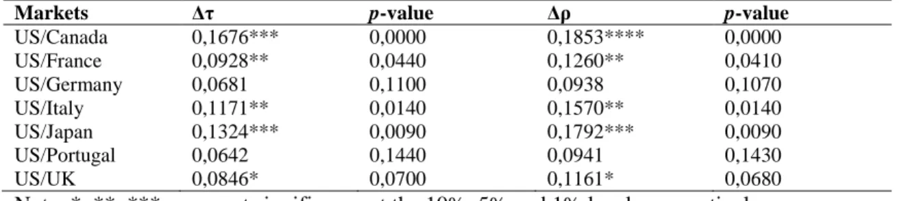
and ρ are directly comparable for distinct copulas and they are therefore the coefficients utilised in the formal tests of contagion.Table 1 below, displays the results for the test of financial contagion in the subprime crisis. Recall that the null hypothesis is the absence of contagion (H0:∆τ ≤0). One thousand replicas were performed in the bootstrap procedure (R=1000). In each of the replicas, the obtained values for ∆τ (and ∆ρ) were ordered, leading to a probability function for ∆τ (and ∆ρ). This function was subsequently used to calculate the p
values which result from a unilateral test, reflecting the left area of probability of 0
= ∆τ .
Table 1. Testing financial contagion in the subprime crisis
Markets ∆τ p-value ∆ρ p-value
US/Canada 0,1676*** 0,0000 0,1853**** 0,0000 US/France 0,0928** 0,0440 0,1260** 0,0410 US/Germany 0,0681 0,1100 0,0938 0,1070 US/Italy 0,1171** 0,0140 0,1570** 0,0140 US/Japan 0,1324*** 0,0090 0,1792*** 0,0090 US/Portugal 0,0642 0,1440 0,0941 0,1430 US/UK 0,0846* 0,0700 0,1161* 0,0680
Note: *, **, *** represent significance at the 10%, 5% and 1% levels, respectively.
The test’s results based on the Kendall’s
τ
and on the Spearman’s ρ are qualitatively identical. For a 10% significance level, five markets exhibit evidence of contagion from the US crisis: Canada, Japan, France, Italy and the UK. The null hypothesis could not be rejected for the German market (though the values are close to rejection, with a p value of 0,1070 for the test based on the Spearman’s ρ). The null is clearly not rejected in the case of the Portuguese market, thus suggesting that more15
peripheral markets (perhaps less exposed to the toxic products associated with the subprime crisis) were at first more shielded against the crisis’ contagious effects. In fact, Canada, the closest market to the focus of the crisis also displays the highest level of contagion.
According to what could be anticipated, the markets exhibiting the highest levels of dependence towards the US before the crisis are also those which display clearer signs of financial contagion afterwards. In the pre-crisis period, the markets exhibiting more synchronized co movements with the US are, in decreasing order of the
Spearman’s ρ: Canada (0,6097), Italy (0,4378), France (0,4359), Germany (0,4323), the UK (0,4215), Japan (0,3297) and Portugal (0,2097). This order is almost unchanged if countries are ordered by the p values resulting from the test on the existence of
contagion: Canada (0,0000), Japan (0,0090), Italy (0,0140), France (0,0410), the UK (0,0680), Germany (0,1070) and Portugal (0,1430).
Within the European markets presenting similar dependence levels in the pre-crisis period (see the copula parameters’ estimates in Table 3.B), the German market appears to be the most prepared to resist the crisis, as it presents the weakest signs of contagion (non-significance at the 10% significance level). On the other hand, the Japanese market, in spite of displaying a less intense dependence with the US before the crisis, appears to be one of the most vulnerable to the crisis effects.
With the results of the first test suggesting that some markets are more affected than others, test 2 is developed to formally assess such hypothesis. This is done by evaluating whether the differences in contagion intensity are statistically significant. Table 2 displays this test’s results.
16
Table 2. Testing contagion intensity in the subprime crisis
Country B
∆τA-B Canada France Germany Italy Japan Portugal UK
Country A Canada 0,0748 0,0995* 0,0505 0,1273 0,1034* 0,0830 France 0,0247 -0,0243 -0,0396 0,0286 0,0082 Germany -0,0940 -0,0643 0,0039 -0,0165 Italy -0,0153 0,0529 0,0325 Japan 0,0682 0,0478 Portugal -0,0204 UK
Note: * represents significance at the 10% level.
The first number on the first raw represents the disparity between the difference of the
τ
for the US/Canada pair, between the pre-crisis and the crisis period, and that of the US/France pair: 0,0748 = (0,5996 – 0,4320) – (0,3918 – 0,2990).In spite of the various positive figures in the table, suggesting that market A has been more intensely affected than market Bvii (with the negative figures indicating the
opposite), the null hypothesis of homogeneous intensity is only rejected, and at a 10% significance level, for the pairs Canada/Germany and Canada/Portugal. The Canadian market is thus the only one exhibiting stronger levels of contagion. However, even in these cases, it should not be stated that there is evidence of higher contagion intensity, as the German and the Portuguese markets did not exhibit signs of contagion in the first test. In the sake of precision, it is more appropriate to conclude that contagion intensity in the Canadian market is stronger than the increases in dependence experienced by the German and the Portuguese markets towards the US’s in the first months following the beginning of the subprime crisis.
17
Conclusions
This study used MSCI daily data for the Portuguese and the G7 countries’ stock markets to assess financial contagion from the subprime crisis in the seven months following the burst of the mortgage bubble. Adopting the copula methodology to model dependence between the US and each of the other markets in the sample, two tests developed with two measures of rank correlation derived from the copulas, the Kendall’s
τ
and the Spearman’s ρ, are performed to formally identify the existence of contagion and to check the homogeneity of contagious effects across markets.The results of the first test suggest that the Canadian, the Japanese, the Italian, the French and the UK markets display significant signs of contagion. Such evidence could not be found for the German and, mainly, for the Portuguese markets. In these two cases it is therefore more correct to simply acknowledge an increase in dependence towards the US market. In fact, though the values of the rank correlation coefficients in the pre-crisis and in the crisis periods augmented, the increase was not sufficient to produce a rejection of the null hypothesis of no contagion.
The second test checks whether contagion intensity differs across markets. The results suggest that only the Canadian market appears to be more intensely affected and solely if confronted with the two markets for which no evidence of contagion could be found, Portugal and Germany. It should thus be concluded that the intensity of
contagion displayed by the Canadian market is statistically higher than the increase in the interdependence registered for the German and Portuguese markets with the US, from the pre-crisis, to the crisis period, and is similar to that of the remaining countries.
18
The two tests were developed using rank correlation coefficients and not the copulas’ dependence parameters because the later are not always comparable. However, the information on the copulas selected to characterise the links between the US and each of the markets in the sample may also supply relevant information. For instance, the fact that the t Student copula was identified as the most adequate in the pre-crisis period and the Frank copula appears to be better fitted for the crisis period, suggests that almost all selected copulas present a symmetric structure, in contrast with the results of Longin and Solnik (2001), Ang and Chen (2002), and Ang and Bakaert (2002).
The results also show that markets displaying higher levels of dependence in the pre-crisis period present more robust evidence of contagion afterwards. The Portuguese market displays no significant signs of contagion, eventually as a result of its more peripheral economic profile. Amongst the European markets presenting similar dependence levels in the pre-crisis period, the German market appears to be the most prepared to resist the effects of the crisis, at least at this early stage. In contrast, the Canadian and the Japanese markets exhibit the strongest signs of vulnerability, with evidence of contagion significant at the 1% level.
The conclusions of this empirical analysis may be useful in various contexts, the most obvious probably being that of portfolio management. Our results suggest that simple strategies of geographical diversification may not be the best solution to
diversify risk. The links between markets in periods of relative financial stability should also be taken into account as they frequently point to their most likely behaviour in times of crisis. More proximate markets, that may preferred by investors attracted by their familiarity and similarity with their domestic circumstances may be inappropriate
19
choices, running the risk of adding similar types of risk to a portfolio and jeopardising the advantages of diversification.
Tests of financial contagion have also been used to evaluate the adequateness of interventions by central banks in previous critical circumstances. In the particular case of the subprime crisis, our results suggest that contagion was clearly present in the Canadian, Japanese and UK markets, justifying an early intervention and the supply of liquidity by the respective central banks. The case of the European Central Bank is less straightforward, at this light, because the evidence of contagion amongst its members was, at an early stage, mixed. However, the reported distress signs on the part of relevant financial institutions, and the behaviour of the rank correlation coefficients in all analysed cases, indicate that intervention was needed to prevent worst case scenarios.
References:
Ang, A. and G. Bakaert (2002), ‘International asset allocation with regime shifts’, Review of Financial Studies, 15 (4), 1137-1187.
Ang, A. and J. Chen (2002), ‘Asymmetric correlations of equity portfolios’, Journal of Financial Economics, 63 (3), 443-494.
Bae, K., G. Karolyi and R. Stulz (2003), ‘A new approach to measuring financial contagion’, Review of Financial Studies, 16 (3), 716-763.
Boyer, B., M. Gibson and M. Loretan (1999), ‘Pitfalls in tests for changes in correlations’, Board of Governors of the Federal Reserve’s International Finance Discussion Paper 597.
20
Cappiello, L., B. Gerard and S. Manganelli (2005), ‘Measuring co movements by regression quantiles’, European Central Bank Working Paper 501.
Clayton, D. (1978), ‘A model for association in bivariate life tables and its application in epidemiological studies of familial tendency in chronic disease incidence’, Biometrika, 65 (1), 141-151.
Corsetti, G., M. Pericoli and M. Sbracia (2005), ‘Some contagion, some interdependence: more pitfalls in tests of financial contagion’, Journal of International Money and
Finance, 24 (8), 1177-1199.
Costinot, A., T. Roncalli and J. Teïletche (2000), ‘Revisiting the dependence between financial markets with copulas’, SSRN Working Paper, available at:
http://ssrn.com/abstract=1032535
Dias, A. (2004), Copula inference for finance and insurance, Doctoral Thesis ETH No. 15283, Swiss Federal Institute of Technology, Zurich.
Embrechts, P., F. Lindskog and A. McNeil (2003), ‘Modelling dependence with copulas and applications to risk management’, in S. Rachev (ed), Handbook of Heavy Tailed Distributions in Finance, Elsevier, pp. 331-385.
Fisher, R. (1932), Statistical Methods for Research Workers, London, Oliver & Boyd. Forbes, K. and R. Rigobon (2001), ‘Measuring contagion: conceptual and empirical
issues’, in S. Claessens and K. Forbes (eds), International Financial Contagion, Kluwer Academic Publishers, pp 43-66.
Frank, M. (1979), ‘On the simultaneous associativity of F(x,y) and x+y – F(x,y)’, Aequationes Mathematicae, 19 (1), 194-226.
Gonzalo, J. and J. Olmo (2005), ‘Contagion versus flight to quality in financial markets’, Universidad Carlos III de Madrid’s Economic Series Working Paper 05-18.
21
Gumbel, E. (1960), ‘Distributions des valeurs extremes en plusieurs dimensions’, Publications de l’Institute de Statistique de l’Université de Paris, 9, 171-173.
Lee, L. (1983), ‘Generalized econometric models with selectivity’, Econometrica, 51 (2), 507-512.
Longin, F. and B. Solnik (2001), ‘Extreme correlation of international equity markets’ Journal of Finance, 56 (2), 649-676.
McLeish, D. and C. Small (1988), The Theory and Applications of Statistical Inference Functions, NewYork: Springer-Verlag.
McNeil, A. and P. Embrechts (2005), Quantitative Risk Management: Concepts, Techniques and Tools, Princeton University Press.
Misiti, M., Y. Misiti, G. Oppenheim and J. Poggi (1997), Wavelet Toolbox for Use with MATLAB, The MathWorks Inc.
Nelsen, R. (2006), An Introduction to Copulas, New York: Springer.
Patton, A. (2002), Applications of Copula Theory in Financial Econometrics, PhD Dissertation, University of California, San Diego, available at:
https://www.amstat.org/sections/bus_econ/papers/patton_dissertation.pdf
Rodriguez, J. (2007), ‘Measuring financial contagion: a copula approach’, Journal of Empirical Finance, 14 (3) 401-423.
Schmidt, T. (2006), ‘Coping with copulas’, in Rank, J. (ed.), Copulas: from theory to application in finance, Risk Books.
Sklar, A. (1959), ‘Fonctions de repartition à n dimensions et leurs marges’, Publications de l’Institute de Statistique de l’Université de Paris, 8, 229-231.
22
Trivedi, P. and D. Zimmer (2005), ‘Copula modelling: an introduction for practitioners’, in P. Trivedi and D. Zimmer (eds), Foundations and Trends in Econometrics, Now Publishers Inc., pp. 1-111.
ANNEX A:
Step 1: Elimination of autoregressive and conditional heteroskedastic effects
In order to make sure that the first period is in fact a pre-crisis period, the series of returns built with the distinct indices were decomposed to the scale 1, using a wavelet of Haar, as suggested by Misiti et al. (1997), and the main structural break occurred near the burst of the mortgage bubble was confirmed.
To eliminate trend dependence effects in the series, the procedures suggested inter alia by Dias (2004) and Gonzalo and Olmo (2005) were adopted. Firstly, through and analysis of the autocorrelation functions and of the Ljung-Box-Pierce and Engle’s ARCH tests, the problems of temporal dependence were assessed in means and in variances. Using the Box-Jenkins’ method, ARMA models were estimated for each return’s average.viii
GARCH (1,1) models were adjusted for the volatilities.
After estimating the ARMA-GARCH models, the filtered returns were recuperated. The tests previously described were again developed to assess whether the identified
problems were corrected.
23
Table 1.A: Estimated ARMA-GARCH models
Index Model
Canada ARMA(0,0)-GARCH(1,1)
France ARMA(1,1)-GARCH(1,1)
Germany ARMA(1,1)-GARCH(1,1)
Italy ARMA(0,1)-GARCH(1,1), C=0 fixed
Japan ARMA(0,0)-GARCH(1,1), C=0 fixed
Portugal ARMA(0,0)-GARCH(1,1)
UK ARMA(0,0)-GARCH(1,1)
24
ANNEX B:
Table 1.B: Distribution functions for the univariate series of filtered returns
Pre-crisis period Selected distribution Log likelihood AIC µ-location parameter σ-location parameter νννν-deg freedom Canada Logistic 878,79 -1753,58 0,0281 (0,0376) 0,5439 (0,0179) - France Logistic 881,51 -1759,01 0,0097 (0,0368) 0,5370 (0,0177) - Germany Logistic 884,62 -1765,24 0,0179 (0,0367) 0,5373 (0,0178) - Italy Logistic 877,35 -1750,70 0,0261 (0,0366) 0,5348 (0,0177) - Japan Logistic 845,47 -1686,94 0,0208 (0,0374) 0,5352 (0,0181) - Portugal t loc-scale 862,81 -1719,63 -0,0152 (0,0348) 0,7716 (0,0358) 5.5743 (1,1540) UK Logistic 884,95 -1765,90 0,0024 (0,0378) 0,5469 (0,0180) - US Logistic 871,67 -1743,30 0,0622 (0,0359) 0,5260 (0,0174) - Crisis period Selected distribution Log likelihood AIC µ-location parameter σ-location parameter νννν-deg freedom Canada Logistic 219,57 -435,13 0,0116 (0,0896) 0,6208 (0,0434) - France Gaussian 221,28 -438,56 -0,2185 (0,0915) 1,1053 (0,0650) - Germany Logistic 214,27 -424,55 -0,1460 (0,0865) 0,5994 (0,0419) - Italy Extreme value 214,72 -425,43 0,3344 (0,0874) 0,9586 (0,0599) - Japan t loc-scale 205,40 -406,80 -0,1400 (0,0928) 0.9867 (0,0978) 10.9886 (9,4228) Portugal Logistic 215,20 -426,39 -0,2371 (0,0846) 0,5908 (0,0410) UK Gaussian 218,43 -432,86 -0,1090 (0,0910) 1,0952 (0,0646) - US Gaussian 224,24 -444,48 -0,0691 (0,0933) 1,1279 (0,0663) - Notes: Logistic function: mean equal to the location parameter and variance equal to π2/3σ2. If X follows a t location-scale distribution with ν>2 degrees of freedom, (X- µ)/ σ follow a t-Student distribution with mean and variance equal to zero and ν/(ν-2), respectively.
Extreme Value distribution: mean equal to µ+γ* σ, where γ is the Euler’s constant, and variance equal to
π*σ2/6.
25
Table 2.B: Adjusted copulas (pre-crisis period)
Copula models Dependence parameters Weight parameters AIC
θθθθ1 θθθθ2 θθθθ3 w1 w2 w3 US/Canada: Clayton 0,9004 - - - - - Gumbel 1,7099 - - - -294,3 Frank 4,3987 - - - -270,1 Gaussian 0,6277 - - - -314,3 t-Student 0,6262 - - - -313,0 Clayton-Gumbel 1,1387 1,7625 - 0,2715 0,7285 - -299,7 Gumbel-Survival Gumbel 1,7461 1,6719 - 0,5998 0,4002 - -301,9 Clayton-Gumbel-Frank 1,1083 1,7500 22,9375 0,2711 0,7130 0,0159 -295,8 US/France: Clayton 0,5838 - - - -134,5 Gumbel 1,4382 - - - -153,1 Frank 2,8755 - - - -126,4 Gaussian 0,4672 - - - -155,7 t-Student 0,4525 - - - -169,2 Clayton-Gumbel 0,6738 1,4662 - 0,3431 0,6569 - -162,7 Gumbel-Survival Gumbel 1,4675 1,3767 - 0,5394 0,4606 - -164,1 Clayton-Gumbel-Frank 0,7197 1,4688 -99,9375 0,3393 0,6513 0,0094 -161,9 US/Germany Clayton 0,5652 - - - -133,7 Gumbel 1,4354 - - - -149,5 Frank 2,8904 - - - -125,8 Gaussian 0,4599 - - - -151,0 t-Student 0,4488 - - - -165,4 Clayton-Gumbel 0,4867 1,5977 - 0,4423 0,5577 - -161,6 Gumbel-Survival Gumbel 1,6731 1,2502 - 0,4716 0,5284 - -161,1 Clayton-Gumbel-Frank 0,5280 1,5883 -100,0000 0,4345 0,5600 0,0055 -159,2 US/Italy Clayton 0,5487 - - - -131,6 Gumbel 1,4539 - - - -153,4 Frank 2,8616 - - - -125,7 Gaussian 0,4660 - - - -154,1 t-Student 0,4544 - - - -161,8 Clayton-Gumbel 0,5081 1,5742 - 0,4008 0,5992 - -161,2 Gumbel-Survival Gumbel 1,6094 1,2783 - 0,5180 0,4820 - -161,6 Clayton-Gumbel-Frank 0,5649 1,5625 -99,9375 0,3844 0,6070 0,0086 -158,8 US/Japan Clayton 0,4563 - - - -97,0 Gumbel 1,3027 - - - -82,8 Frank 2,1449 - - - -69,6 Gaussian 0,3911 - - - -100,7 t-Student 0,3761 - - - -100,6 Clayton-Gumbel 0,4700 1,3985 - 0,6277 0,3723 - -102,3 Gumbel-Survival Gumbel 1,3892 1,2581 - 0,2940 0,7060 - -99,8 Clayton-Gumbel-Frank 0,4700 1,3985 2,0420 0,6278 0,3722 0,1252 -98,3 US/Portugal Clayton 0,2580 - - - -33,2 Gumbel 1,1418 - - - -22,2 Frank 1,3132 - - - -27,4 Gaussian 0,2160 - - - -28,8 t-Student 0,2192 - - - -33,6 Clayton-Gumbel 0,1952 2,1250 - 0,8880 0,1120 - -33,4 Gumbel-Survival Gumbel 1,0938 1,1875 - 0,2866 0,7134 - -30,8 Clayton-Gumbel-Frank 0,1954 2,7656 1,7188 0,8025 0,0723 0,1252 -19,8 US/UK: Clayton 0,5354 - - - -114,5 Gumbel 1,4200 - - - -145,0 Frank 2,7234 - - - -115,8 Gaussian 0,4508 - - - -141,8 t-Student 0,4378 - - - -152,1 Clayton-Gumbel 0,5840 1,4580 - 0,2988 0,7012 - -148,7 Gumbel-Survival Gumbel 1,4581 1,3438 - 0,6195 0,3805 - -150,0 Clayton-Gumbel-Frank 3,9141 1,4063 -1,5000 0,0806 0,8793 0,0401 -144,5
26
Table 3.B: Adjusted copulas (crisis period)
Copula models Dependence parameters Weight parameters AIC
θθθθ1 θθθθ2 θθθθ3 w1 w2 w3 US/Canada Clayton 1,8387 - - - -126,1 Gumbel 2,3654 - - - -131,1 Frank 8,4777 - - - -143,0 Gaussian 0,7812 - - - -133,9 t-Student 0,8087 - - - -149,6 Clayton-Gumbel 1,5615 3,2969 - 0,3919 0,6081 - -148,4 Gumbel-Survival Gumbel 3,7023 1,9999 - 0,4487 0,5513 - -149,1 Clayton-Gumbel-Frank 1,3027 3,0000 17,0000 0,3763 0,2322 0,3925 -149,4 US/France Clayton 0,6077 - - - -30,2 Gumbel 1,5689 - - - -43,3 Frank 4,1226 - - - -50,2 Gaussian 0,5072 - - - -41,4 t-Student 0,5383 - - - -43,3 Clayton-Gumbel 9,9193 1,4609 - 0,1346 0,8654 - -44,4 Gumbel-Survival Gumbel 1,4424 7,2802 - 0,8702 0,1298 - -44,0 Clayton-Gumbel-Frank 11,921 1,0313 5,0000 0,0854 0,2060 0,7086 -46,4 US/Germany Clayton 0,5683 - - - -26,4 Gumbel 1,4976 - - - -35,4 Frank 3,6899 - - - -41,7 Gaussian 0,4745 - - - -34,7 t-Student 0,5058 - - - -37,1 Clayton-Gumbel 0,9944 1,5245 - 0,2945 0,7055 - -34,3 Gumbel-Survival Gumbel 1,5017 1,5414 - 0,6400 0,3600 - -33,8 Clayton-Gumbel-Frank 0,0005 2,3594 4,2266 0,1322 0,0763 0,7915 -34,1 US/Italy Clayton 0,6661 - - - -27,5 Gumbel 1,5494 - - - -42,2 Frank 4,4063 - - - -53,6 Gaussian 0,5408 - - - -45,5 t-Student 0,5507 - - - -43,9 Clayton-Gumbel 4,3335 1,5216 - 0,1928 0,8072 - -43,8 Gumbel-Survival Gumbel 1,6269 1,6504 - 0,6455 0,3545 - -42,6 Clayton-Gumbel-Frank 9,5434 1,4063 4,5000 0,0578 0,1639 0,7783 -46,6 US/Japan Clayton 0,5183 - - - -23,5 Gumbel 1,5574 - - - -45,4 Frank 3,4463 - - - -35,5 Gaussian 0,5169 - - - -40,6 t-Student 0,5182 - - - -39,0 Clayton-Gumbel 0,9095 1,5574 - 0,0000 1,0000 - -41,4 Gumbel-Survival Gumbel 1,5574 1,6550 - 1,0000 0,0000 - -41,4 Clayton-Gumbel-Frank 0,9095 1,5574 2,8875 0,0000 1,0000 0,0000 -37,4 US/Portugal Clayton 0,2157 - - - -3,5 Gumbel 1,2161 - - - -8,5 Frank 1,9094 - - - -11,4 Gaussian 0,2701 - - - -9,1 t-Student 0,2701 - - - -7,1 Clayton-Gumbel 0,0891 1,2813 - 0,2105 0,7895 - -4,4 Gumbel-Survival Gumbel 1,1563 2,7188 - 0,8787 0,1213 - -5,7 Clayton-Gumbel-Frank 4,8571 1,0302 1,6314 0,0635 0,0000 0,9365 -4,0 US/UK: Clayton 0,5720 - - - -29,8 Gumbel 1,5054 - - - -36,8 Frank 3,8021 - - - -44,0 Gaussian 0,5089 - - - -41,5 t-Student 0,5089 - - - -39,5 Clayton-Gumbel 0,4158 2,0000 - 0,4853 0,5147 - -37,4 Gumbel-Survival Gumbel 2,0469 1,2656 - 0,4645 0,5355 - -36,8 Clayton-Gumbel-Frank 50,000 1,0005 3,6978 0,0402 0,0307 0,9291 -40,7
27
Table 4.B: Selected Copulas
US/Canada US/France US/Germany US/Italy US/Japan US/Portugal US/UK Pre-crisis period
Selected Copula Gaussian t-Student t-Student t-Student Clay.-Gumb. t-Student t-Student
Dep. Param. (θ1) 0,6277 (0,0249) 0,4525 (0,0373) 0,4488 (0,0366) 0,4544 (0,0350) 0,4700 (0,0718) 0,2192 (0,0395) 0,4378 (0,0351) Dep. Param. (θ2) - - - - 1,3985 (0,1844) - - Weight Parm. (w1) - - - - 0,6277 (0,1333) - - Weight Param. (w2) - - - - 0,3723 (0,1333) - - Kendall’s τ 0,4320 (0,2040) 0,2990 (0,0267) 0,2963 (0,0261) 0,3003 (0,0250) 0,2255 ((0,0236) 0,1407 (0,0258) 0,2885 (0,0248) Spearman’s ρ 0,6097 (0,2510) 0,4359 (0,0366) 0,4323 (0,0359) 0,4378 (0,0343) 0,3297 (0,0329) 0,2097 (0,0379) 0,4215 (0,0343) Crisis Period
Selected Copula t-Student Frank Frank Frank Gumbel Frank Frank Dep. Parameter (θ) 0,8087 (0,0369) 4,1226 (0,6461) 3,6899 (0,6324) 4,4063 (0,6063) 1,5574 (0,1154) 1,9094 (0,5424) 3,8021 (0,6472) Kendall’s τ 0,5996 (0,0390) 0,3918 (0,0469) 0,3644 (0,0490) 0,4174 (0,0425) 0,3579 (0,0477) 0,2049 (0,0539) 0,3731 (0,0500) Spearman’s ρ 0,7950 (0,0384) 0,5619 (0,0605) 0,5261 (0,0648) 0,5948 (0,0541) 0,5089 (0,0623) 0,3038 (0,0779) 0,5376 (0,0661) Note: Standard deviations in brackets.
28
Endnotes:
i Forbes and Rigobon, 2001, p. 44.
ii See, for instance, Embrechts et al. (2002) and Cherubini et al. (2004).
iii In this study, bivariate continuous copulas are used, as the focus of the analysis is the structure of dependence between pairs of markets.
ivRandom drawing of 2000 points departing from the copula of: (1) Clayton, with θ = 1.5; (2) Clayton, with θ = 3; (3) Gumbel, with θ = 2; (4) Gumbel, with θ = 3. It was assumed that the marginal variables
X1 (in the horizontal axis) and X2 (vertical axis) follow standardized Gaussian distributions.
v Due to the different time zones, working hours in Japan and in the US do not overlap. Therefore, in order to ensure that the information contained in the US index is reflected in the Japanese index only in the next working day, the series of US data is lagged.
vi
For instance, the intervals for
θ
in the Clayton and in the Gumbel copula, are[
0,+∞]
and[ ]
1,+∞ , respectively.vii For example, the table’s first raw suggests that the Canadian market is the most affected, since all the elements in the first raw are positive.
viii An augmented Dickey-Fuller test is used to test for the absence of unit roots in the series and, therefore, to assess the adequacy of the proposed methods of analysis.
ix As the dimension of the series is variable (following the elimination of the holidays), and since the object of the assessment is the dependence towards the US, the size of each series was adjusted to that of the US and the ARMA-GARCH model for the US index presents small variations.