Participating life annuities incorporating longevity risk sharing arrangements

Texto

(1)Participating life annuities incorporating longevity risk sharing arrangements¤ Jorge Miguel Bravoy. Pedro Corte Realz. Carlos Pereira da Silvax. September 2009. Abstract In this paper we develop a conceptual framework for the payout phase in which annuity providers and policyholders share longevity and investment risks in a ‡exible way. To be more precise, we develop an participating life annuity product in which systematic longevity risk, i.e., the risk associated with systematic deviations from mortality rates extracted from prospective life tables derived for the Portuguese population, is shared between both counterparties. This will address some of the main demand and supply constraints in annuity markets, namely the inexistence of prospective life tables for the Portuguese population, the perception of unfair pricing, the consideration of bequest motives, adverse selection problems or the lack of …nancial instruments to hedge against longevity risk. Contrary to traditional GSA’s, in which surviving policyholders bear both systematic and unsystematic longevity risk, we devise a contract in which, in exchange for a relatively small premium, annuitants will bear only the part of longevity that exceeds pre-determined thresholds. JEL Code: G19, G22, G23 Keywords: longevity risk; annuities; a¢ne models; stochastic mortality; longevitylinked derivatives. ¤ Paper prepared for submission to the scienti…c contest Prémio Inovação Reforma – Programa Consciência Leve, promoted by Grupo Caixa Geral de Depósitos. y University of Évora - Department of Economics and CEFAGE-UE / CIEF, Largo dos Colegiais, N. 2, 7000-803, Évora/Portugal, Tel.: +351 266 740894, E-Mail: jbravo@uevora.pt. z Universidade Nova de Lisboa – Faculdade de Ciências e Tecnologia x ISEG - Universidade Técnica de Lisboa. 1.

(2) Contents 1 Introduction 1.1 Demographic trends . . . . . . . . . . . 1.2 Financial implications of longevity risk . 1.3 Options for the Payout-Phase . . . . . . 1.4 Main constraints facing annuity markets 1.5 Modeling mortality and longevity risk .. . . . . .. . . . . .. . . . . .. . . . . .. . . . . .. . . . . .. . . . . .. . . . . .. . . . . .. . . . . .. . . . . .. . . . . .. . . . . .. . . . . .. . . . . .. 4 6 7 8 10 13. 2 Group Self Annuitization life annuities 14 2.1 Risk pooling principle . . . . . . . . . . . . . . . . . . . . . . . . . 14 2.2 Annuity portfolio losses . . . . . . . . . . . . . . . . . . . . . . . . 19 3 Deriving Prospective Lifetables for Portugal 3.1 Notation, assumptions and quantities of interest 3.2 Mortality projection method . . . . . . . . . . . . 3.3 Modelling the time-factor . . . . . . . . . . . . . 3.4 Data . . . . . . . . . . . . . . . . . . . . . . . . . 3.5 Results . . . . . . . . . . . . . . . . . . . . . . . . 3.5.1 Parameter estimates . . . . . . . . . . . . 3.5.2 Extrapolating time trends . . . . . . . . . 3.5.3 Projecting the mortality for the oldest-old: 3.5.4 Mortality Projections . . . . . . . . . . . 3.5.5 Life expectancy . . . . . . . . . . . . . . . 3.5.6 Annuity prices . . . . . . . . . . . . . . .. . . . . . . . . . . . . . . . . . . . . . . . . . . . . . . . . . . . . . . . . . . . . . . . . . . . . . . . . . . . . . . . . . . . . . . Closing Lifetables . . . . . . . . . . . . . . . . . . . . . . . . . . . . . .. 21 21 22 27 27 29 29 31 32 33 37 41. 4 A¢ne-Jump di¤usion processes for mortality 42 4.1 Mathematical framework . . . . . . . . . . . . . . . . . . . . . . . . 42 4.2 Mortality intensity as a stochastic process . . . . . . . . . . . . . . 44 4.3 Calibration to the Portuguese projected lifetables . . . . . . . . . 46 5 Participating life annuity with longevity risk sharing mechanism 48 5.1 5.2. Structure of the contract . . . . . . . . . . . . . . . . . . . . . . . . Simulations . . . . . . . . . . . . . . . . . . . . . . . . . . . . . . .. 6 Conclusion. 48 50 52. 2.

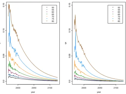
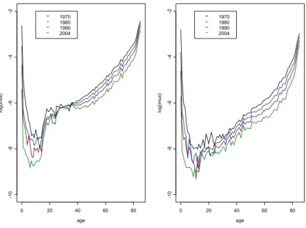
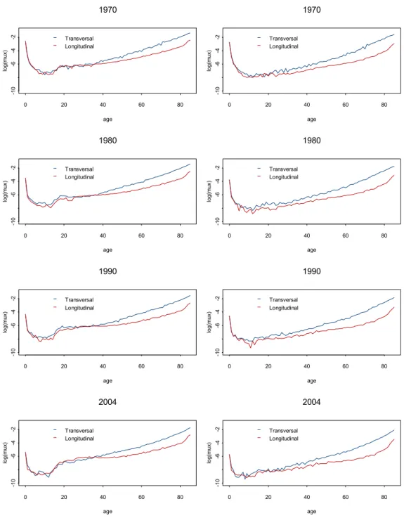
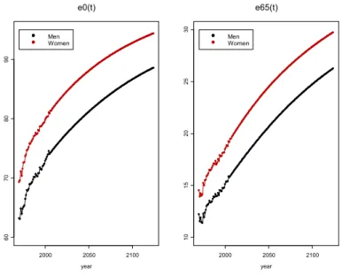
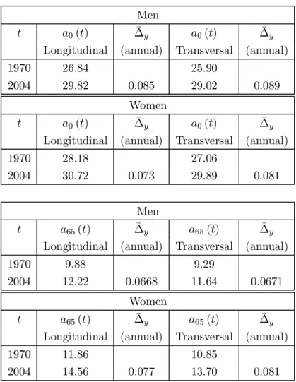
(3) List of Tables 1 2 3 4 5 6. Estimation of the parameters of the ARIMA(p,d,q) models . . . . Evolution of life expectancy at birth and at age 65 calculated according to both a transversal and diagonal approach . . . . . . . . Evolution of  () for  = 0 and  = 65 . . . . . . . . . . . . . . . Parameter estimates . . . . . . . . . . . . . . . . . . . . . . . . . . Simulated premiums (cohort size 1.000) . . . . . . . . . . . . . . . Simulated premiums (cohort size 10.000) . . . . . . . . . . . . . . .. 31 39 41 47 51 52. List of Figures 1 2 3 4 5 6 7 8 9 10 11 12 13. Crude mortality rates for the period 1970-2004, males . . . . . . . Crude mortality rates for the period 1970-2004, females . . . . . . Estimations of     and  for men (left panels) and women (right panels). . . . . . . . . . . . . . . . . . . . . . . . . . . . . . . . . . Estimated and projected values of  with their 95% con…dence intervals for males (left panel) and females (right panel) . . . . . . Mortality rates for closed lifetables, males . . . . . . . . . . . . . . Mortality rates for closed lifetables, females . . . . . . . . . . . . . Evolution of  () for men (left panel) and women (right panel) . Evolution of  for some representative ages, from 1970 to 2124, for men (left) and women (right) . . . . . . . . . . . . . . . . . . . Evolution of the instantaneous force of mortality for some representative generations for men (left panel) and women (right panel) Transversal vs cohort approach, for selected calendar years, for men (left panel) and women (right panel) . . . . . . . . . . . . . . . . . Life expectancy  () calculated at  = 0 65 for men (left panel) and women (right panel) . . . . . . . . . . . . . . . . . . . . . . . . Projected life expectancy at birth and at age 65, calculated according a transversal approach . . . . . . . . . . . . . . . . . . . . . . . Survival probability  ¡ 65 () as a function of age  +  ¡  for  = 1970 and  = 2004 (the left panel corresponds to the male population) . . . . . . . . . . . . . . . . . . . . . . . . . . . . . . .. 3. 28 28 30 32 34 34 35 35 36 38 40 40. 48.

(4) 1 Introduction Longevity risk, i.e., the risk that members of some reference population might live longer, on average, than anticipated, has recently emerged as one of the largest sources of risk faced by individuals, life insurance companies, pension funds and annuity providers. This risk is ampli…ed by the current problems in de…ned bene…t (DB) pension systems (either PAYGO …nanced or funded and public or private), in which the amount of retirement bene…ts is determined largely by years of service, that will inevitably force the systems to moderate bene…t promises in the future. Additionally, the international pension environment is shifting towards de…ned contribution (DC) systems, in which retirement wealth depends on how much individuals save and how successfully they allocate their assets accumulated in DC plans, forcing individuals to be much more aware and active in managing this risk. The e¢cient allocation of these assets requires the managing of a number of risks, such as the investment risk, timing of annuitization and longevity risk (i.e. the possibility of exhausting assets before passing away). It also depends on the existence of solutions to manage both …nancial and demographic risks, on the regulatory environment and on type of options and products available. If in recent years pension discussions were mainly focused on questions such as system design or on ways to encourage saving in the accumulation phase, the design of the payout phase and the di¤erent retirement options for DC plans will soon be at the center of the debate. The main problem will be on how to encourage certain retirement payout options in order to guarantee that people will have appropriate retirement income and longevity protection, while considering liquidity, health-care costs or bequest motives. The regulatory implications of the guarantees o¤ered to retirees will need to be balanced so that capital reserves required (e.g., life insurance companies) in excess of what can be fairly and profitably delivered by private providers don’t result in the lack of products or in ine¢cient allocation of resources. Assets accumulated in DC pension plans may be allocated in the payout phase in three alternative ways: lump-sum payments, programmed withdrawals, and annuities, although we can envisage mixed arrangements involving any combination of these. With lump-sums, individuals receive the entire value of the assets accumulated for retirement as a single payment. Under programmed withdrawals, individuals establish a schedule of periodic …xed or variable payments. Finally, “plain vanilla” life annuities involve a constant stream of income paid at some regular interval for as long as the individual lives. The main factors that di¤erentiate. 4.

(5) between these options are the degree of ‡exibility and exposure to investment risk versus the degree of protection against longevity risk. The main purpose of this project is to develop a conceptual framework for the payout phase in which annuity providers and policyholders share longevity and investment risks in a ‡exible way. To be more precise, we develop an participating life annuity product in which systematic longevity risk, i.e., the risk associated with systematic deviations from mortality rates derived using prospective life tables for the Portuguese population, is shared between both counterparties. This will address some of the main demand and supply constraints in annuity markets, namely the inexistence of prospective life tables for the Portuguese population, the perception of unfair pricing, the consideration of bequest motives, adverse selection problems or the lack of …nancial instruments to hedge against longevity risk. We hope the results of this project will contribute to the development of an e¢cient annuity market in Portugal. The paper is organized in four main parts. In Section 1 we brie‡y review the main demographic trends observed worldwide and discuss the macroeconomics and …nancial implications of longevity risk. Next, we discuss the type of retirement payout options for accumulated assets in savings accounts or DC pensions, emphasizing the importance of annuity markets in protecting individuals from longevity risk. Next, we discuss the main demand and supply constraints undermining the development of annuity markets in Portugal and in most OECD countries. Finally, we brie‡y introduce traditional and stochastic mortality approaches in mortality modelling. In Section 2 we analyse in detail the main features of a special type of participating life annuity called Guaranteed (or pooled) Self Annuitization (GSA) annuity fund. The advantages and limitations of this contract in hedging longevity risk are highlighted in comparison with standard “plain vanilla” annuities. In Section 3 we derive the …rst prospective lifetables for the Portuguese population. This provides us with new tools for the analysis of mortality trends, namely the possibility to investigate the evolution of mortality not only in terms of calendar time but also in terms of year of birth or cohort. In Section 4 we use stochastic di¤erential equations to model the random evolution of survival probabilities. Speci…cally, we propose (and calibrate) a new SDE for the force of mortality. The model is then embedded into an a¢ne-jump term structure framework in order to derive closed-form solutions for the survival probability, a key element when pricing life insurance contracts. In Section 5 we develop a new participating life annuity with a longevity risk sharing mechanism. Section 6 concludes. 5.

(6) 1.1 Demographic trends It is well documented that the population of the industrialized world underwent a major mortality transition over the last decades. Improved hygiene and living standards, breakthrough medical progresses, generally healthier lifestyles, the absence of both major pandemic crisis and global military con‡icts have created the conditions for individuals to enjoy raising life expectancy at all ages. Based on all available demographic databases, historical trends show that both average and the maximum lifetime have increased gradually during the last century, with human life span showing no signs of approaching a …xed limit imposed by biology. In Portugal, life expectancy at birth increased from 48.08 (52.12) years in 1930-31 to 75.49 (81.74) in 2006-08 for the male (female) population. As in other developed countries, the mortality decline has been dominated by two major trends: a huge reduction in mortality due to infectious diseases a¤ecting mainly young ages, more evident during the …rst half of the century, and a decrease in mortality at older ages, more pronounced during the second half. As a consequence, the number of those surviving up to older ages (e.g., 80 years and above) has increased signi…cantly representing, in 2006, 4.9% (2.9%) of the Portuguese female (male) population. Additionally, the number of deaths of the oldest-old accounts for an increasing proportion of all deaths, with reductions of mortality beyond these ages having a growing contribution to future gains in life expectancy. Decreasing mortality at old ages raised longevity to values considered impossible in the past. In Portugal, life expectancy at age 65 raised from11.49 (13.09) years in 1930-31 to 16.25 (19.61) years in 2006-08. The general downward trend in mortality rates at almost all ages means that an increasing proportion of the members of a given generation lives up to very old ages (around 75-85 years), shifting the survival function upwards and to the right to a more rectangular shape in what is know in the literature as the rectangularization phenomena. At the same time, we can observe that the age of maximum mortality gradually shifted towards older ages, in what is sometimes called the expansion phenomenon of the survival curve. At the same time, fertility rates are declining. Recent data shows that while in 1960 each Portuguese woman gave birth to 3.1 children on average, nowadays the ratio in only 1.4, far below the threshold of around 2.1 necessary to keep the population of a developed country constant. In fact, in Portugal as in many developed countries low fertility rates are, together with increasing life expectancy, the main drivers of an ageing population. The immediate consequence of higher life expectancy and low fertility rates 6.

(7) in unambiguous. According to the United Nations, in 2050 27% of the European population will be older than 65 years (16% in 2005) and around 10% will be older than 85 (compared with 3.5% in 2005). This has important consequences in terms of population mix, as can be seen, for example, by looking at the evolution of young-age and old-age dependency ratios. In Portugal, the young-age dependency ratio has been cut by more than half from 46.0 in 1960 to 22.8 in 2007. In opposite direction, the old-age dependency ratio has increased steadily from 15.6 in 1970 to 25.9 in 2007. Considering the ageing (or vitality) index, while in 1970 there were 34 old people for each young people, in 2007 this relation has dramatically shifted to 114 old for 100 young people.. 1.2 Financial implications of longevity risk Mortality improvements are naturally viewed as a positive change for individuals and as a substantial social achievement for developed countries. Nonetheless, the combination of longer life and low fertility rates poses a huge challenge to both societies and individuals since they are now exposed to increasing longevity risk. Macroeconomics e¤ects of population ageing range from impacts on labour supply and its rate of utilization to investment, productivity and saving/consumption patterns, external balances and cross-border capital ‡ows, consumer preferences and corporate strategies, health-care and social security systems. In the insurance market, mortality improvements have an obvious impact on the pricing and reserving for any kind of long-term living bene…ts, particularly on annuities. The demographic scenario described above is also driving to important changes in the income mix of retirees. First, as a consequence of a rising old-age dependency ratio, the number of wage and salary earners is becoming insu¢cient to fund a growing number of retirees. Traditional PAYGO social security systems will progressively become unsustainable and will require substantial reforms. Alternative solutions involve an increase in the contribution rates, a reduction in pension/salary replacement rates, an increase in retirement age, a search for new funding sources. Changes in public pension systems are likely to imply, ceteris paribus, a noteworthy reduction in the retirement income relative to wages. i.e., a relative reduction in state-provided pension income. Second, there is a clear market trend away from de…ned-bene…t (DB) corporate pension schemes to de…ned-contribution (DC) schemes. In these arrangements, retirement bene…ts are largely determined by how much workers save and how successfully they allocate their assets accumulated in DC plans. The e¢cient allocation of these assets requires the managing of risks, such as the timing of 7.

(8) annuitization and longevity risk, i.e., the possibility of outliving one’s retirement income. It also depends on the type of options and products available and on the regulatory environment. This means that employer-related pension bene…ts could equally become more uncertain in the future. Third, the extended mobility of the workforce has broken down traditional family networks, thus reducing in practice the ability of younger members of a family to take care of the older ones, the main source of intergenerational solidarity mechanism in the past. The changing pattern observed in labour markets towards more ‡exible and less stable arrangements will probably induce erratic social security contribution patterns, essentially dependent on salaries pro…les over time. This said, individuals will have to become in a near future more self-reliant and will want to supplement and diversify their sources of income in retirement, assigning greater weight to private solutions and increasing the ‡ow of saving allocated to fund retirement. In addition, increases in life expectancy will probably not be followed by an equivalent upward adjustment in the retirement age and thus individuals will have to put aside an increasing proportion of their lifetime income in order to fund their extended lifetime. Moreover, increases in life expectancy have consistently exceeded forecasts, i.e., individuals are faced with longevity risk, something that must also be considered in order to ensure that the elderly do not experience drops in consumption.. 1.3 Options for the Payout-Phase Given the importance of addressing retiree’s needs in their …nancial needs, both in their accumulation and decumulation (or payout) phases, in this section we brie‡y review the main retirement options available for the payout-phase. Individuals with assets accumulated in DC plans or individual saving accounts have roughly three main options for the payout phase: lump-sum payments, programmed withdrawals and annuities. Combined solutions involve any possible combination between these three alternatives are of course possible. With lump-sums, individuals simply receive the entire value of the assets accumulated for retirement as a single payment. That amount can then be freely allocated, for example, to buy discretionary items, to pay down debts, to buy annuities, to cover for contingencies (e.g., medical expenses). Under programmed withdrawals, individual agree on a set of periodic payments (…xed or variable), which can be determined on di¤erent ways (e.g., by dividing the accumulated capital by a …xed number of years) and allow for some ‡exibility, for example to adjust for unexpected contingency payments. Finally, a traditional whole life 8.

(9) annuity is a stream of income payments paid at some regular interval for as long as individual lives. The main factors that di¤erentiate between these options are the degree of ‡exibility versus the degree of protection from longevity risk. Lump-sum payments are fully ‡exible and provide complete liquidity, allowing individuals to dispose and allocate their wealth as they wish, including the option to leave bequests. However, lump-sum payments do not provide protection from outliving one’s own resources, i.e., individuals bear in this case all longevity risk. According to life-cycle theory, in a world with no uncertainty rational individuals would save optimally and, on retirement, would merely allocate their wealth by spreading assets over their remaining years of life, so as to ensure optimal retirement consumption (and cover bequest motives, if any). In a dynamic environment, future life expectancy is unknown and as such individuals are faced with the prospect of outliving their expected life spans. In a scenario of unknown longevity, individuals rely heavily on …nancial discipline to manage their resources. Retirees can reduce the risk of exhausting assets before passing away by consuming less per year, but such a tactic then increases the chance that they might die with too much wealth left unconsumed. In other words, dying with too little wealth is undesirable, but having too much wealth is also undesirable, since it represents foregone consumption opportunities. Programmed withdrawals provide more …nancial discipline than lump-sums, while maintaining some degree of ‡exibility, access to liquidity and the possibility to cover bequest motives, but fail once again to provide any kind of protection from longevity risk. Finally, life annuities o¤er full protection against longevity risk, but at least in their "plain vanilla" form, are in‡exible and illiquid and do not provide for bequest motives. Nevertheless, in some countries annuity markets o¤er today a wide range of complex annuity products, including embedded guarantees that protect against interest rate, in‡ation, market volatility, and early death, accommodate liquidity and contingency payments and o¤er tax advantages. However, up to now little attention has been devoted to the development of annuity products in which mortality and longevity risks are shared and payouts linked to the evolution of demographic variables. In this paper tackle this problem and develop an annuity product in which mortality and longevity risks are shared between annuitants and life insurance companies. The decision as to which of these three main retirement payout options is preferred relies mostly on individual preferences, the type of pension arrangements 9.

(10) in place, the “generosity” of PAYGO pension systems, as measured for example by the replacement rates, the availability of other sources of income in retirement, tax incentives, the existence of individual account type systems, …nancial education, mandatory annuitization constraints or the level of development of insurance markets. Overall, the life insurance industry should be prepared to help retirees to meet their …nancial needs, both in the accumulation and payout phases. In the accumulation phase, companies should help individuals to build up a desired level of savings throughout their working years in a ‡exible and e¢cient way. In a ‡exible way, assisting individuals to choose the amount and timing of their contributions to the capitalisation plan. In an e¢cient way via, for example, investment diversi…cation strategies, gradual adjustment of the risk/return pro…le according to age, tax incentives. As to the decumulation phase, life insurance companies have a crucial role in allowing individuals to have access and run their asset pool in a ‡exible and smooth way, while o¤ering protection against longevity, in‡ation and investment risks. This can be done by o¤ering various types of annuities, with alternative payout mechanisms (…xed or variable, in‡ation-linked, equity-linked, participating arrangements, additional embedded guarantees), through health care and longterm care insurance or through wealth monetisation (e.g., reverse mortgages) for those whose assets are not in liquid form.. 1.4 Main constraints facing annuity markets Life annuity products have been sold in the past primarily as retirement accumulation vehicles, rather than decumulation products (Brown et al., 2001). This may explain why annuity markets in Portugal and in most OECD countries have been relatively underdeveloped to date. However, annuity markets su¤er from a wide range of demand and supply constraints1 . On the demand side, limitations to the development of annuity markets include, …rst, the level of annuitization from PAYGO-…nanced pensions, i.e., the degree on which annuities are crowded out by social security provision and the degree on which they are crowded out by other forms of pension saving such as DB occupational schemes. Second, annuities are perceived to be unfairly priced, mostly because life insurance companies do not fully disclose information on the technical basis used to calculate annuity premiums. Third, the motive to bequest assets on death to dependents is not covered by “plain vanilla” annuities. Fourth, the demand for annuities is determined to 1. For a detailed discussion on this subject see, for example, Stewart (2007) and Rusconi (2008).. 10.

(11) some extent by personal considerations such as family support, the need to cover the costs of unexpected medical expenses, the inexistence of su¢cient liquid assets to purchase an annuity or liquidity concerns. For example, for older people, the risk of having to pay large medical bills or cover special health care costs induces them to retain at least a fraction of their assets instead of annuitising them. Fifth, …scal incentives are considered insu¢cient to stimulate insurance protection against longevity risk. In modern competitive markets, individual …nancial decisions are also driven by people’s perceptions about the appeal of alternative investments, both during their working lifetime and after retirement. For instance, some individuals may avoid annuitisation on the grounds that they can manage their assets better than institutional fund managers. In this scenario, introducing tax incentives (or tax-favoured competing assets) could undermine saving decisions in favour of buying annuity protection. Finally, in some cases there is a general mistrust of institutions providing annuities. On the supply side, the type and scope of the limitations to the development of annuity markets is also signi…cant. First, high-quality information on mortality tables depicting a particular group’s distribution of expected remaining lifetime is required. Projected mortality tables should take into consideration the stochastic nature of the remaining lifetime and encompass cohort e¤ects. Uncertainty regarding mortality tables can cause insurance companies to prices annuities conservatively, exacerbating adverse selection problems and lowering the access to the market. Additionally, uncertainty regarding mortality data can cause individuals to seriously underestimate their survival prospects, which, in turn, can lead them to undervalue the importance of longevity insurance. Dissemination of mortality should, in this sense, be considered a matter of public interest and form part of a clear supervision policy. In Portugal, there are not regulatory lifetables (neither contemporaneous lifetables nor prospective lifetable) either for the Portuguese overall population or for life insured populations. As a result, life insurance companies are forced to use as their technical basis lifetables adopted in other countries. Although this practice is authorized by the supervising authorities, using a survival law drawn up from other population’s experience, potentially biased when compared to the demographic conditions observed in Portugal, involves signi…cant basis risks, in particular the risk of overestimating the mortality risk of the population. In Section 3 we address this issue and derive the …rst prospective lifetables for the Portuguese general population. Second, annuity markets are often a¤ected by strong adverse-selection problems. This arises if buyers of annuities prove to be live longer than average, 11.

(12) inducing insurance companies to devise separate mortality tables for annuitants as opposed to those for the general population. The existence of adverse selection problems induces companies to include signi…cant margins when pricing for annuity contracts. Whether adverse selection is quantitatively important may depend on whether annuitisation is considered optional or mandatory. In this sense, increasing compulsory annuitisation can signi…cantly reduce adverse-selection problems. Third, the potential for growth in annuity markets cannot be fully accommodated if insurance companies lack assets with which to back the long-term promises represented by annuities. Appropriate asset types either do not exist or are available in insu¢cient quantity. Insurance companies o¤ering annuity products are faced with two major risk sources: interest-rate risk and longevity risk. Standard immunisation theory suggests that in order to protect themselves from small changes in the term structure of interest rates, insurance companies should back their annuity portfolios with assets whose respective durations equal those of the annuity liabilities, and whose respective convexities are larger than those of the annuity liabilities. This is di¢cult in practice, since long-term bonds are not available in most bond markets. Moreover, if real annuities are to be provided, real long-term bonds will have to be issued as well. This means that annuity markets would de…nitely bene…t from the issuance of long-term government bonds. Moreover, recent events in Argentina and Russia have shown that the quality of assets considered is important, since the possibility of default is real. On the other hand, longevity risk, i.e., the chance that entire cohorts live longer than anticipated in projected mortality tables, remains a real concern for insurance companies selling annuity products, since substantial changes in mortality patterns could seriously challenge their pro…tability. Insurance companies can, for example, hedge longevity risk with o¤setting life insurance contracts, reducing (but not eliminating completely) the impact of negative mortality scenarios. Some advocate that governments (or private companies) should issue cohort “survivor bonds” (or longevity bonds), i.e., bonds whose future coupons payments depend on a survivorship index (for example, the percentage of the whole population of retirement age - say 65 - on the issue date still alive on the future coupon payment dates).2 Although survivor bonds are good candidates for hedging aggregate mortality risk, they do not provide a perfect hedge against the particular characteristics of a company’s pool of annuitants. In this sense, there is basis risk between the 2. See, e.g., Blake and Burrows (2001) and Blake et al. (2006a).. 12.

(13) reference population mortality and the mortality experienced by any individual pool of annuitants. Other problems related to the issuance of survivor bonds include: i) the ability of dealing with a business involving huge amounts of capital, ii) pricing complications related to the adoption of a particular (stochastic) representation of mortality uncertainty and the estimation of the market price of longevity risk and iii) the importance of attractive contract design in order to boost market liquidity for traded securities and reduce credit risk. Once a well organised and liquid market for survivor bonds is in place, a whole new avenue is open for the development of survivor-derivative products (for example, mortality options based on a certain mortality index, futures contracts based on survival forecasts, survivor swaps interchanging cash ‡ows based on two di¤erent mortality experiences, longevity forwards3 ). Finally, alternative methods of hedging longevity risk include the use of traditional reinsurance methods, or through risk-sharing in the capital markets, which are particularly attractive for investors because of the low or negative correlation with traditional risk factors such as …nancial market indexes, or through the option of annuity securitisation, which would bene…t insurance companies by providing them with alternative means for ooading their mortality improvements risk exposure. Fourth, traditional annuity markets are incomplete in the sense that do not offer protection against in‡ation, they lack equity market exposure, they are illiquid and do not insure against multiple shocks. Finally, there are concerns regarding regulatory capital requirements or with the strength of existing providers that would make it di¢cult for new entrants to survive. In order to address these problems, many policy options exist to encourage and promote annuity markets. Examples include mandating annuitization, improving …nancial literacy, dealing with longevity risk or producing longevity indexes.. 1.5 Modeling mortality and longevity risk One of the key conditions for the development of longevity-linked products and markets and for the hedging of longevity risk is the development of generally agreed market models for risk measurement. Whereas traditional market risks such as equity market, interest rate, exchange rate, credit and commodity risks have well consolidated methodologies for quantifying risk-based capital and for establishing market prices, longevity and mortality risk has historically been a very opaque risk. For a long time, only demographers, actuaries and insurance 3. For a detailed discussion see, e.g., Blake et al. (2006a,b) and Bravo (2007).. 13.

(14) companies showed any interest in measuring and managing this risk, mainly for pricing purposes. A number of explanations can be given for this, particularly the fact that it is a non-…nancial risk that has been measured and analyzed in a di¤erent way from …nancial risks, generally adopting deterministic or scenario based approaches. Historically, actuaries have been calculating premiums and mathematical reserves using a deterministic approach, by considering a deterministic mortality intensity, which is a function of the age only, extracted from available (static) lifetables and by setting a ‡at (“best estimate”) interest rate to discount cash ‡ows over time. Since neither the mortality intensity nor interest rates are actually deterministic, life insurance companies are exposed to both …nancial and mortality (systematic and unsystematic) risks when pricing and reserving for any kind of long-term living bene…ts, particularly on annuities. In particular, the calculation of expected present values requires an appropriate mortality projection in order to avoid signi…cant underestimation of future costs. In order to protect the company from mortality improvements, actuaries have di¤erent solutions, among them to resort to projected (dynamic or prospective) lifetables, i.e., lifetables including a forecast of future trends of mortality instead of static lifetables. Static lifetables are obtained using data collected during a speci…c period (1 to 4 years) whereas dynamic lifetables incorporate mortality projections. In a situation where longevity is increasing over time, static lifetables underestimate lifelengths and thus premiums relating to life insurance contracts. Conversely, dynamic lifetables will project mortality into the future accounting for longevity improvements. Since the future mortality is actually unknown, there is enormous likelihood that future death rates will turn out to be di¤erent from the projected ones, and so a better assessment of longevity risk would be one that consists of both a mean estimate and a measure of uncertainty. Such assessment can only be performed using stochastic models to describe both demographic and …nancial risks. In the following sections, we review both the traditional “dynamic approach” and the new “stochastic mortality approach”.. 2 Group Self Annuitization life annuities 2.1 Risk pooling principle Through “plain vanilla” annuities, life insurers o¤er their policyholders protection against two broad classes of risk: biometric risks, such as longevity and mortality 14.

(15) risks, and macroeconomic and …nancial market risks, such as interest rate, in‡ation, equity market or credit market risk. In this kind of product insurers bear all risk, both systematic (e.g., longevity risk, the risk that people systematically live longer than predicted) and unsystematic or idiosyncratic risk (e.g., …nancial market volatility, mortality deviations around predicted values,...). To introduce a special type of participating life annuity called Guaranteed (or pooled) Self Annuitization (GSA) annuity fund consider the following simple example. Let us take a group of ten 90-year-old Portuguese women, who are concerned about outliving their …nancial wealth over the next year. Statistically, the latest estimations show that there is an approximately 20% probability of death in the next year. To protect against longevity risk, they agree to contribute EUR 100 to a common fund, which will redistribute the capital and investment return (say 5% yield pa) amongst survivors. At the end of the year each of them will get between EUR 105 (if no-one dies) and EUR 1050 (if nine out of ten die), based on actual mortality experience. What this example highlights is that by pooling mortality risk and ceding bequest, individuals seem to all gain. In fact, ex-ante all fund participants receive some protection against longevity risk over the duration of the contract. If the agreement between the ten old ladies were to be intermediated by an insurance company, involved a large number of people, and lasted for the remaining lifetime of participants’ lives, it would constitute a special type of participating life annuity called Guaranteed Self Annuitization annuity fund. Through this kind of arrangement, with a large investment pool, and assuming that longevity risk is null, the funds contributed by those who die earlier than expected on the basis of expected mortality rates are "inherited" by those who survive and supplement the pool’s capital market gains, o¤ering thus a larger bene…t than could be achieved through individual investments. Stated more formally, consider a standard GSA annuity fund.4 Without loss of generality, the pool starts (at time  = 0) with an initial size of  homogeneous insured persons in the sense of identical age, gender and cohort, identical monetary amounts and identical risk exposures. We assume that contracts are sold to policyholders in exchange for a single upfront premium 0  given exogenously throughout the entire analysis. The contract provides a ‡at bene…t 0 paid once a year. Given these assumptions and the best estimate of future mortality, the 4. For a comprehensible introduction GSA’s see, for instance, Piggott and Detzel (2004) and Richter and Weber (2009).. 15.

(16) starting total fund is 0 =  0  Ä. (1). where  Ä is the standard actuarial notation for the present value of whole life annuity-due, determined using the mortality information and projections available at time  = 0 and assuming a constant discrete interest rate of  per period (we will use the year as the period, any generalizations can be made using the usual approaches, e.g., interpolation). Such a pure annuity provides a unit payment for the remaining lifetime of an insured person initially aged , i.e., contingent on the insured’s survival. Using the equivalence premium principle, Ä is given by 0 1 () 1 X X ©  ª A @  =  ¢  (2)  Ä = E =0. =0. where  = () = [ ()] is the number of completed future years lived by (), also denominated the curtate future lifetime of  (see, for instance, Gerber [1997]), and where  = (1 + )¡1 denotes the standard discount factor. This starting total fund can also be considered the initial total reserve, i.e., 0 = 0  In a GSA, the future value of annuity bene…ts remains constant over the whole contract unless deviations from expected mortality rates are observed. If that is not the case, i.e., if the number of those surviving up to higher ages is di¤erent form expected, the remaining reserves have to be redistributed among the remaining survivors. Assuming that realized investment rates will be as expected5 , the total fund at time  = 1 comprises the initial value less annuity payments accrued at the technical interest rate 1 = 1 = (0 ¡  0 ) (1 + ). (3). ± Redistributing this reserve among the actual +1 remaining survivors for their. expected future lifetime, including the reserves “inherited” from non-surviving members, the future value of annuity bene…ts becomes, after some algebra µ ¶ 1  1 = ± = 0 (4) +1 ± where  and ± denotes, respectively, the expected and realized survival probabilities for an individual aged  at time  = 0 in the time interval (  + 1) 5. The extension to the case where the realized investment earnings pattern is di¤erent from the assumed constant rate  is straightforward (see, e.g., Piggott et al., 2004). 16.

(17) Proceeding inductively, at any time  in the future the bene…t payment will be determined by µ ¶    = 0 (5) ±  . From (5) it is clear that future annuity payments depend on the ratio of survivorship rates. In a scenario of longevity risk, i.e., in a scenario where the number of those surviving to age  +  is systematically higher than initially expected bene…t payments will inevitably drop in order to prevent fund imbalance. This contrasts with traditional life annuity contracts that guarantee a level payment for the remainder of recipient’s lifetime independently of future mortality developments. From (5) it also clear that bene…t payments at time  can be expressed as 8   > > < min (0   )   ¤  1   0  (6)  ( ) = ¤ = 1   > > : max (0   )   ¤  1  . For instance, in a scenario of longevity risk the bene…t payment is given by the ± current value of the reference fund distributed among the actual +1 remaining survivors capped by its inception value 0  This bene…t can be expressed in terms of the …nal (maturity) payo¤ of an European put option with strike equal to the annuity bene…t at inception, i.e.,  () = 0 ¡ max f0 ¡ ; 0g. (7). If, for the contrary, actual remaining survivors are less than initially estimated, bene…t payments at time  are ‡oored by the annuity bene…t at inception and can be expressed in terms of the …nal payo¤ of an European call option with strike equal to 0 , i.e.,  () = 0 + max f ¡ 0 ; 0g (8) Equations (8) and (7) show that GSA annuity contracts include option features that, up to our knowledge, have never been considered in the design and pricing of these contracts. In fact, insurance companies adopt an over-simpli…ed approach and completely ignore embedded options, resorting to consolidated actuarial techniques for pricing (and hedging) the contract. After all, in a GSA annuity fund all actual losses/pro…ts are beared by the remaining survivors, whose bene…ts ‡uctuate according to mortality developments. However, this solution may have a disastrous e¤ect from a marketability point 17.

(18) of view. For example, in a scenario of longevity risk future bene…ts will decrease and this may spread discontent through those who weren’t aware of the potential impact of future mortality improvements on their “apparently guaranteed” income and may feel they didn’t receive any compensation for being short in put option contract. Compared to standard life annuities, policyholders in a GSA may question the fact that insurance companies don’t pay a premium for the option to cut back annuity payments in case of adverse mortality improvements. On the other hand, if actual longevity developments are worst than initially expected, bene…t payments in a GSA will increase due to a higher “inheritance e¤ect” or “survivor bonus” since the accumulated funds will be spread across a smaller surviving group. Compared to standard life annuities, in this case life insurance companies will not be compensated for the “lost” reserves. Individuals assessing the possibility of annuitizing their wealth but disbelief about their longevity prospects may feel attracted to buy an GSA annuity contract type if given the chance to increase annuity payments if their prospects con…rm. Moreover, in this case life insurance companies may sell a separates call options on future bene…t payments, upgrading thus the value of the overall line of business. Although the framework of GSA is interesting at a theoretical level it as no practical interest in life insurance competitive markets for a number of reasons. Firstly, as in other variable annuity contracts the annuitant does not know in advance the rate of return of the pool, hence it carries some risk. In particular, GSA without additional guarantees are structured so that individuals share both mortality and investment risk in upside and downside times. Second, annuitants can see theirs payments dropping below a reasonable value in the presence of longevity risk. Third, there will be no payments for lives above the technical limit of the mortality table used to …rst price annuities, i.e., individuals might end up with no resources to fund consumption. Fourth, insurance companies (or fund’s manager) does not bear any kind of risk, either actuarial or …nancial, either systematic of idiosyncratic. In fact, this is a simple approach to the di¤usion of risk since, in the classical framework of GSA, there is no need to use a risk bearer (as an insurer or fund’s manager) since the funds are periodically reallocated to the annuitants, based on the previous payment adjusted for any deviations in mortality and interest from expectations. Fifth, in its simplest form, a GSA does not give pool member’s access to the principal investment nor to any accumulated fund. This means that the product does not cover legacy motives. Finally, buyers of such product tend to be people who expect to live longer, raising once again the question of adverse selection. 18.

(19) The apparent advantage of GSA’s over self-insuring is that the risk exposure is not immediate in that is borne by the pool and it’s smoothed out by the insurance company over a long time horizon. In addition, since mortality and investment are largely uncorrelated, there is some chance that a negative return on investments may be partially o¤set by a positive “inheritance e¤ect” or vice-versa. In other words, the e¤ects of the overall risk exposure might be mitigated and postponed at the individual level when considered in a pooling structure. To address these concerns, we propose in Section 5 a new participating life annuity contract in which mortality and longevity risks are shared between policyholders and insurance companies. The contract includes option-like features that adjust bene…ts if future mortality developments are signi…cantly di¤erent from expected.. 2.2 Annuity portfolio losses A di¤erent way to understand the option-like features of annuity contracts is to analyse the relation between survival probabilities and annuity portfolio losses. Consider a classic life annuity contract with level payment 0 . The loss on the underlying annuity portfolio at time  is de…ned as  =.  X =1. ( ()0 ¡ E [ ()0 ])+. (9). where  () = 1   is an indicator function that jumps from 1 to 0 at the time of death   of the annuitant. Note that E [ ()] =   Losses on the portfolio are the amount that the annuity payments at time  exceed the expected payments. For a given population survival probability   , the distribution of the number alive at time  is binomial + » B (   ) j . (10). As recognized by Lin and Cox (2005), there are two sources of uncertainty in the portfolio loss at time  This …rst is due to uncertain lifetimes given the actual mortality rates. The second is attributed to the stochastic nature of survival probabilities. Given this, the total variability in the portfolio is the unconditional variance of the compound binomial distribution   (+ ) = E [  [(+ ) j ]] +   [E [(+ ) j  ]]. 19. (11).

(20) For large portfolios of annuitants, the main source of uncertainty will come from changes in mortality rates impacting all lives in the portfolio rather than the variability in the number of deaths at a particular age given the mortality rate. In other words, the randomness in + will mainly be due to the uncertainty in    Life insurance companies pool mortality risks by the Law of Large Numbers, i.e., lim !1 E [  [(+ ) j  ]] ! 0 However, from (11) we can conclude that the assumption that mortality and longevity risks can be diversi…ed away by writing a large number of policies in incorrect if we take into account the dynamics of the underlying mortality rates, i.e.,   [E [(+ ) j  ]] 6= 0 Mortality dynamics is in‡uenced by a complex setting of socioeconomic factors, biological variables, government policies, environmental e¤ects, health conditions and social behaviours. Since the future mortality is actually unknown, there is always the likelihood that future death rates will turn out to be di¤erent from the projected ones and thus mortality shocks can destroy the insurance pooling mechanism. For example, for an annuity portfolio the risk is that the annuitants will systematically live longer than expected at the policies inception. Systematic mortality risk cannot be eliminated by diversi…cation and thus should have a market price. The portfolio loss in equation (9) can be written as  =  0 [ ± ¡  ]+ Redistributing among the remaining survivors we have ·µ ± ¶ ¸    0 ±   ¡  + ;0 = ± [  ¡  ] = 0 max ± ± + +   ·µ ¶ ¸   = 0 max 1 ¡ ± ; 0  . (12). (13). Equation (13) shows that the loss "inherited" by each surviving policyholder includes an option feature that depends on ratio of survivorship rates. To be more speci…c, the loss has an embedded put option with strike equal to unity and underlying equal to the ratio between estimated and actual survivorship rates. To value this option we can resort to traditional discrete-time (Binomial) or continuous-time approaches (Black-Scholes), with proper adjustments for an. 20.

(21) incomplete markets situation. Alternatively, we can resort to Monte-Carlo simulation techniques.6. 3 Deriving Prospective Lifetables for Portugal In this section we derive prospective lifetables for the Portuguese general population. The results are then compared with that of classical static lifetable approach to give an indication of the longevity risk currently faced by portuguese insurance companies.. 3.1 Notation, assumptions and quantities of interest The basic idea underlying projected lifetable methods is to analyse changes in mortality as a function of both age  and time . Let  () denote the force of mortality at age  during calendar year . Let  () and  () = 1 ¡  () represent, respectively, the one-year death probability at age  in year  and the corresponding survival probability. Let  denote the number of deaths recorded at age  during year  from an exposure-to-risk (i.e., the number of person years from which  arise)   Consider now the classic Lexis diagram, that is, a coordinate system that has calendar time as abscissa and age as coordinate. If we assume that both time scales are divided into yearly bands, the Lexis plane is partitioned into squared segments. In this paper, we assume that the age-speci…c forces of mortality are constant within bands of time and age, but authorized to change from one band to the next. Formally, given any integer age  and calendar year , we assume that + ( +  ) =  () for any 0 ·    1 (14) In other words, assumption (14) means that mortality rates are constant within each square of the Lexis diagram, but allowed to vary between squares. From (14) the calculation of the probability of an individual aged  in year ,  ()  and of the corresponding death probability  () = 1 ¡  () simpli…es to  () = exp (¡ ()) = 1 ¡  (). (15). Several markers are regularly used by demographers to measure the evolution of mortality, namely life expectancies, variance of residual lifetime, median lifetime 6 The valuation of options embedded in GSA funds is being performed in an accompanying paper.. 21.

(22) or the entropy of a lifetable. Let º  () denote the (complete) life expectancy of an -aged individual in year  i.e., the average number of years he is expected to survive. This means we expect this individual will die in year  +º  () then aged  +º  () Contrary to classic static lifetables, the use of projected lifetables allows us to estimate the “true” (diagonal) expected residual lifetime of an individual. The appropriate formula for º  () is given by 9 8  = X <Y + ( + ) º  () = ; : ¸0. =0. 1 ¡ exp (¡ ()) =  () 9 8 ¡ ¢ X <¡1 Y ¡ ¢= 1 ¡ exp ¡+ ( + ) exp ¡+ ( + ) + ; : + ( + ) ¸1. (16). =0. The actual computation of º  () requires the knowledge of  ( ) (or  ( )) for  ·  ·  and  ·  ·  +  ¡  where  denotes the ultimate (maximum) age. Since these survival probabilities are knot known at time  they have to be estimated using extrapolation methods based on past trends. The next section gives an example of how this can be done in practice. For life insurance companies and annuity providers, the net single premium of an immediate life annuity sold to an -aged individual in year   ()  is of special interest. In a dynamic approach, the appropriate formula for  () is given by 8 9  = X <Y  () = + ( + ) +1 (17) : ; ¸0. =0. where  = (1 + )¡1 is the classic discount factor considering a ‡at term structure.. As can be seen, mortality projections and projected survival probabilities are particularly important to price correctly annuity and other life insurance contracts.. 3.2 Mortality projection method The literature on the construction of projected lifetables is vast and growing.7 The classical approach is to …t an appropriate parametric function (e.g. Makeham model) to each calendar year data. Then, each of the parameter estimates is treated as independent time series, extrapolating their behaviour to the future in order to provide the actuary with projected lifetables (see, e.g., CMIB (1976) and 7 A detailed review of mortality projection methods can be found in Tuljapurkar and Boe (1998), Pitacco (2004), Wong-Fupuy and Haberman (2004) and Bravo (2007).. 22.

(23) Heligman e Pollard (1980)). Despite simple, this approach has serious limitations. In the …rst place, this approach strongly relies on the appropriateness of the parametric function adopted. Secondly, parameter estimates are very unstable a feature that undermines the reliability of univariate extrapolations. Thirdly, the time series for parameter estimates are not independent and often robustly correlated. Although applying multivariate time series methods for the parameter estimates is theoretically possible, this will complicate the approach and introduce new problems. Lee and Carter (1992) developed a simple model for describing the long term trends in mortality as a function of a simple time index. The method models the logarithm of a time series of age-speci…c death rates  () as the sum of an age-speci…c component   that is independent of time, and a second component, expressed as a product of a time-varying parameter denoting the general level of mortality  , and an age-speci…c component   that signals the sensitiveness of mortality rates at each age when the general level of mortality changes. Formally, we have ln  () =  +    +   (18) ¡ ¢ where  » N  0 2 is a white-noise, representing transitory shocks. Parameters  ,   and  have to be constrained by X max.  = 0 and. =min. X max.   = 1. (19). =min. in order to ensure model identi…cation. Parameter estimates are obtained by ordinary least squares, i.e., by solving the following minimization program ) (  X max max X ^   (ln  () ¡  ¡   )2  (20) (^    ^ ) = arg min    . =min =min. Lee and Carter (1992) solve (20) by resorting to Singular Value Decomposition techniques but alternative estimation procedures can be implemented considering iterative methods (see, e.g., Bravo (2007)) or Weighted Least-Squares (see, e.g., Wilmoth (1993)). The resulting time-varying parameter estimates are then modelled and forecasted using standard Box-Jenkins time series methods. Finally, from this forecast of the general level of mortality, projected age-speci…c death rates are derived using the estimated age-speci…c parameters. There have been several extensions to the Lee-Carter model including di¤erent 23.

(24) error assumptions and estimation procedures.8 Bell (1997), Booth et al. (2002a) and Renshaw and Haberman (2003c,d) include a second log-bilinear term in (18) and estimate parameters by considering the …rst two term in a SVD. Additionally, they adopt a multivariate setting in order to project the evolution of the two time indices  ( = 1 2 ) Carter and Prskawetz (2001) consider the possibility of time varying parameters  and   . Renshaw and Haberman (2003a) include additional non-linear age factors when modeling the so-called “mortality reduction factors” within a Generalized Linear Models (GLM’s) approach. Renshaw and Haberman (2006) and Currie et al. (2004) include a cohort factor including year of birth as a factor impacting the rate of longevity improvement. This cohort factor is found to be signi…cant in UK mortality data. Renshaw e Haberman (2005) and Bravo (2007) develop a version of the LeeCarter model considering positive asymptotic mortality. This result is, for most age groups, more consistent with observed mortality patterns when compared with that of the original model. Wilmoth and Valkonen (2002) develop an extension of the Lee-Carter model aimed to investigate di¤erential mortality by considering a number of alternative covariates other than age and calendar time. Cairns, Blake and Dowd (2006b) develop and apply a two-factor model similar to the Lee-Carter model with a smoothing of age e¤ects using a logit transformation of mortality rates. Cairns et al. (2007) analyze England and Wales and US mortality data showing that models that allow for an age e¤ect, a quadratic age e¤ect and a cohort e¤ect …t the data best although the analysis of error distributions in these models revealed disappointing. De Jong and Tickle (2006) formulate the Lee-Carter model in a state space framework. Brouhns et al. (2002a) and Renshaw and Haberman (2003c) develop an extension of the Lee-Carter model allowing for Poisson error assumptions and apply it to Belgian data. This Poisson log-bilinear approach can be stated as  » P ( ()  ) . (21). where  denotes the number of deaths recorded at age  during year  from an exposure-to-risk (i.e., the number of person-years from which  arise), , and  () is given once again by (18). This model has several advantages over the Lee-Carter speci…cation. First, the model doesn’t assume that errors are homoskedastic, an unrealistic assumption since the logarithm of the force of mor8. See Lee (2000), Lee and Miller (2001), Tuljapurkar and Boe (1998), Brouhns et al. (2002a), Wong-Fupuy and Haberman (2004), Bravo (2007) and Cairns et al. (2007) for a detailed discussion of Lee-Carter model and extensions.. 24.

(25) tality is much more variable at older ages that at younger ages. Second, contrary to Lee-Carter model, the Poisson log-bilinear approach doesn’t requires a complete matrix of observed death rates. Finally, one of the main advantages over the Lee-Carter model is that speci…cation (21) allows us to use maximum-likelihood methods to estimate the parameters instead of resorting to least squares (SVD) methods. Formally, we estimate the parameters  ,   and  by maximizing the log-likelihood derived from model (18)-(21) ln V (® ¯ ·) =. X max. X max. =min =min. f ( +    ) ¡  exp ( +    )g +  (22). ¡ ¢0 where ® = (min      max )0  ¯ =  min       max  · = (min      max )0 and  is a constant. The presence of the log-bilinear term    makes it impossible to estimate the model using standard statistical packages that include Poisson regression. Because of this, we resort in this paper to an iterative method proposed by Goodman (1979). The algorithm, which is essentially a Newton-Raphson standard method, states that in iteration  + 1 a single set of parameters is updated …xing the other parameters at their current estimates according to the following updating scheme (+1) () L() ^  = ^  ¡ 2 ()  L  2 (). (23). where L() = L()(^  ) Recall that in our case we have three sets of parameters, corresponding to the     and  terms. (0) ^ (0) (0) The updating scheme is as follows: starting with a given initial vector (^   ^  )  . 25.

(26) then:.  ^ (+1) =  ^ ()   ¡ ^ (+1)  . (+2).  ^. (+1). =  ^. P max. h. ³ í () () ^ ()   ¡  exp  ^ +   ^. =min P max. h ³ í  () () ^ ()  exp  ^ +   ^  . ¡. =. ¡. =min () (+1) ^    ^ P max. (24). h ³ í (+1) (+1) ^ (+1) ^ (+1)   ¡  exp  ^ +  ^  . =min P max. ¡. (). = ^. =min. ³ (+1) ´2 h ³ í  (+1) (+1) ^ ^ (+1)   exp  ^ +  ^  . ^ (+2) =  ^ (+1)  ^ (+2) = ^ (+1)      . ^ (+3) ^ (+2)  =  ¡    ^ (+3) . =. P max. (+1).  ^. =min P max. ¡. =min.  ^ (+2)  . í h ³ (+2) (+2) ^ (+2)  ^  ¡  exp  ^ +  . ³ ´ h ³ í  (+2) (+2) (+2) 2 (+2) ^  ^  exp  ^ +   ^ (+3).  ^. (+2). = ^. We use as a criterion to stop the iterative procedure a very small increase of the log-likelihood function. The maximum-likelihood estimations of the parameters generated by (24) do not match the identi…cation constraints (??), and have thus to be adapted. This is guaranteed by changing the parameterization in the following manner: ¤ = (^  ¡  ¹) . and. where  ¹ denotes average value for  ^  i.e.  ¹=. ^   ¤ = Pmax ^ =min  . (25). X max 1  ^ max ¡ min + 1 = min. and where  is given by =. X max. ^ . =min. from which we …nally calculate. ^  ¤ =  ^ +  ¹ 26. (26).

(27) The new estimates ¤   ¤ and ¤ ful…ll the constraints (??) and provide the ^  ^  since  same  ^ +  ^  = ¤ +  ¤ ¤  Note also that di¤erentiating the loglikelihood function with respect to  yields the equality X .  =. X . ^  = . X . ³ ´ ^  exp  ^ +  ^. This means that the estimated  ’s are such that the resulting death rates applied to the actual risk exposure produce the total number of deaths actually observed in the data for each age .. 3.3 Modelling the time-factor In the Poisson log-bilinear methodology, the time factor  is intrinsically viewed as stochastic process. In this sense, standard Box-Jenkins techniques are used to estimate and forecast  within an ARIMA(  ) time series model. Recall that the model takes the general form (1 ¡ )  =  +. £ ()  © (). (27). where  is the delay operator (i.e.,  ( ) = ¡1  2 () = ¡2    ), 1 ¡  is the di¤erence operator (i.e., (1 ¡ )  =  ¡ ¡1  (1 ¡ )2  =  ¡ 2¡1 + ¡2    ), £ () is the Moving Average polynomial, with coe¢cients µ = ( 1   2        ), © () is the Autoregressive polynomial, with coe¢cients ¡ ¢ Á = 1  2       , and  is white noise with variance 2  The method used to derive estimates for the ARIMA parameters  µ; Á and  is conditional least squares. From these, forecasted values of the time. parameter, denoted by ¤ , are derived. Finally, the parameter estimates of the Poisson model and the forecasts ¤ can be inserted in (??) to obtain age-speci…c mortality rates, prospective lifetables, life expectancies, annuities single premiums and other related markers. In the following we apply the Poisson modelling to Portugal’s general population data in order to derive prospective lifetables.. 3.4 Data The model used in this paper is …tted to the matrix of crude Portuguese death rates, from year 1970 to 2004 and for ages 0 to 84 The data, discriminated by age and sex, refers to the entire Portuguese population and has been supplied by Statistics Portugal(INE - Instituto Nacional de Estatística).. 27.

(28) Figure 1: Crude mortality rates for the period 1970-2004, males. Figure 2: Crude mortality rates for the period 1970-2004, females. 28.

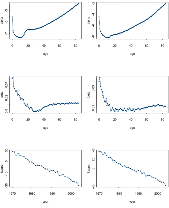
(29) The database for this study comprises two elements: the observed number of death  given by age and year of death, and the observed population size  at December 31 of each year. We follow the INE de…nition of population at risk using the population counts at the beginning and at the end of a year and take migration into account. Figures 1 and 2 give us a …rst indication of mortality trends in Portugal during this period. Two trends dominated the global mortality decline: (i) a reduction in mortality due to infectious diseases, a¤ecting mainly young ages, (ii) decreasing mortality at old ages.. 3.5 Results 3.5.1 Parameter estimates We apply the Poisson modelling to the Portuguese data presented above. The Poisson parameters     and  implicated in (??) are estimated by maximumlikelihood methods using the iterative procedure described in Section ??. We (0) started the updating scheme considering the following initial values  ^  = 0 (0) ^ (0) = 1 and   ^ = 01 The criterion to stop the iterative procedure is a very  small increase of the log-likelihood function (in our case we used 10¡5 ). The routine was implemented within the SAS package. Figure 3 plots the estimated     and  . We note that the  ^  ’s represent the average of the ln  ^  () across the time period. As expected, the average mortality rates are relatively high for newborn and childhood ages, then decrease rapidly towards their minimum (around age 12), increasing then in  re‡ecting higher mortality at older ages. The only exception refers to the well know “mortality hump” around ages 20-25, more visible in the male population, a phenomena normally associated with accident or suicide mortality. We can see that young ages tend to be more a¤ected by changes in the general time trends of mortality, probably due the evolution of medicine in reduc^  ’s decrease with age, except ing infantile and juvenile mortality. In e¤ect, the  for the mortality hump phenomena, but remain positive for all ages. Note also that the sensitiveness of the male population to variations in parameter  tends to be grater than that of the female population, which has a more stable pattern. Finally, we can see that the  ^ ’s exhibit a clear decreasing trend (approximately linear). This reveals the signi…cant improvements of mortality at all ages both for men and women in the last 35 years.. 29.

(30) -2 alpha. -6. -4. -3 -5. alpha. -8. -7 0. 20. 40. 60. 80. 0. 20. 80. 60. 80. 0.03 beta 0.01. beta. 0.02 0.0 0. 20. 40. 60. 80. 0. 20. 40 age. 0 -40. -30. -10. kappa. 10. 20. 30. 40. age. kappa. 60. age. 0.04. age. 40. 1970. 1980. 1990. 2000. 1970. year. 1980. 1990. 2000. year. Figure 3: Estimations of     and  for men (left panels) and women (right panels).. 30.

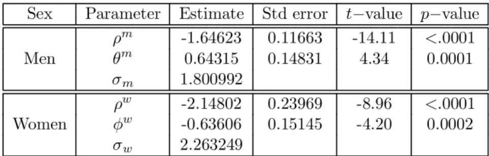
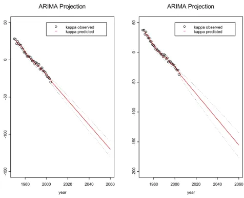
(31) 3.5.2 Extrapolating time trends Let f^    = min      max g denote a realization of the …nite chronologic time series K = f   2 Ng  Following the work of Lee and Carter (1992) and Brouhn et al. (2002a,b), we use standard Box-Jenkins methodology to identify, estimate and extrapolate the appropriate ARIMA (  ) time series model for the male and female time indexes   A good model for the male population is ARIMA(0 1 1), which is a moving average (MA(1)) model     (1 ¡ )   =  +  ¡1 + . (28). whereas for women the ARIMA(1,1,0) autoregressive model was identi…ed as a good candidate     (1 ¡ )  (29)  =  +  ¡1 +   2 2 where   and  are white noise error terms with variance   and    respectively. The estimated parameters for the ARIMA (  ) models (28) and (29) are given in Table 1. Note that all parameters are signi…cant at a 5% signi…cance level.. Sex Men. Women. Parameter      . Estimate -1.64623 0.64315 1.800992 -2.14802 -0.63606 2.263249. Std error 0.11663 0.14831. ¡value -14.11 4.34. ¡value .0001 0.0001. 0.23969 0.15145. -8.96 -4.20. .0001 0.0002. Table 1: Estimation of the parameters of the ARIMA(p,d,q) models. In Figure 4 we show the estimated values of  together with the ¤ projected and the corresponding 95% con…dence interval forecasts.. 31.

(32) 50. ARIMA Projection. 50. ARIMA Projection. kappa observed kappa predicted. -200. -150. -150. -100. -100. -50. -50. 0. 0. kappa observed kappa predicted. 1980. 2000. 2020. 2040. 2060. 1980. 2000. 2020. 2040. 2060. year. year. Figure 4: Estimated and projected values of  with their 95% con…dence intervals for males (left panel) and females (right panel) © ¤ ª Given the forecasted values of   ^ 2004+ :  = 1 2     the reconstituted sex-speci…c forces of mortality are given by ^  ^  (2004 + ) = exp(^  +  ^ ¤2004+ ).  = 1 2   . (30). and then used to generate sex-speci…c life expectancies and life annuities. 3.5.3 Projecting the mortality for the oldest-old: Closing Lifetables According to the United Nations, it is estimated that in 2001 72 million of the 6.1 billion inhabitants of the world were 80 year or older. In the developing world, the population of the oldest-old (e.g., those 80 years and older) still represents a small fraction of the world’s population but it is the fastest growing segment of the population. In addition, because life expectancy will continue to increase, not only we should expect to have an increasing number of people surviving to very old ages, but also anticipate that the deaths of the oldest-old will account for an increasing proportion of all deaths in a given population. In view of this, it is important to have detailed information about the age structure of the oldest32.