JISTEM J.Inf.Syst. Technol. Manag. vol.13 número3

(1)

____________________________________________________________________________________ Manuscript first received/Recebido em: 29/08/2016 Manuscript accepted/Aprovado em: 30/11/2016 Address for correspondence / Endereço para correspondência

Bipul Kumar, Indian Institute of Management, Ranchi Ranchi, India E-mail bippthk22@gmail.com

A NOVEL LATENT FACTOR MODEL FOR RECOMMENDER

SYSTEM

Bipul Kumar

Indian Institute of Management, Ranchi Ranchi, India

______________________________________________________________________

ABSTRACT

Matrix factorization (MF) has evolved as one of the better practice to handle sparse data in field of recommender systems. Funk singular value decomposition (SVD) is a variant of MF that exists as state-of-the-art method that enabled winning the Netflix prize competition. The method is widely used with modifications in present day research in field of recommender systems. With the potential of data points to grow at very high velocity, it is prudent to devise newer methods that can handle such data accurately as well as efficiently than Funk-SVD in the context of recommender system. In view of the growing data points, I propose a latent factor model that caters to both accuracy and efficiency by reducing the number of latent features of either users or items making it less complex than Funk-SVD, where latent features of both users and items are equal and often larger. A comprehensive empirical evaluation of accuracy on two publicly available, amazon and ml-100 k datasets reveals the comparable accuracy and lesser complexity of proposed methods than Funk-SVD.

Keywords: Latent factor model, singular value decomposition, recommender system, E-commerce, E-services, complexity

1. INTRODUCTION

(2)

JISTEM, Brazil Vol. 13, No. 3, Set/Dez., 2016 pp. 497- 514 www.jistem.fea.usp.br

systems collect huge data, process it and project them to aid decision making (Vahidov & Ji, 2005) . Recommender systems are decision support systems used in e-commerce to help navigate customers to the right product (Bauer & Nanopoulos, 2014; Cheung, Kwok, Law, & Tsui, 2003; Chung, Hsu, & Huang, 2013; Ekstrand, 2010; Gan & Jiang, 2013)

Recommender systems assist users by recommending items that can be interesting to users based on their previous buying behaviour (Zou, Wang, Wei, Li, & Yang, 2014). Much of research in recommender systems is primarily influenced by research in information retrieval. Collaborative filtering (CF) is the basic technique implemented in research of recommendation system. Collaborative filtering (CF) method give recommendations of items for users based on patterns of ratings or usage (e.g., purchases) without the need of external information about user or items. More often information about users and/or items is difficult to capture so application of CF as method seems reasonable.

According to Breese, Heckerman, & Kadie (1998) and Yang, Guo, Liu, & Steck (2014), algorithms for collaborative recommendation are grouped into two general classes: memory-based and model-based. Memory based CF method relies on the principle that nearest neighbourhood of users or items correctly represents the user or items that are rated by user and based on the neighbour of users or items recommendations are generated. Model based CF, on the other hand, relies on the principle of building model to predict rating for a user based on past rating. One of the successful model based CF in recommendation system has been matrix factorization (also, known as SVD) which addresses the problem of recommender system, also referred as state-of-art in recommender system (Cremonesi, Koren, & Turrin, 2010; Jawaheer, Weller, & Kostkova, 2014; Konstan & Riedl, 2012).

Recommender systems collect information based on preferences of users on items (movies, news, videos, products etc.). There are two types of category of preferences as expressed by users in literature 1) Explicit feedback 2) implicit feedback. Explicit feedback are those which users directly report their interest on product. For example, Netflix collects star ratings for movies and TiVo users indicate their preferences for TV shows by hitting thumbs-up/down buttons. Because explicit feedback is not always available, some recommenders infer user preferences from the more abundant implicit feedback, which indirectly reflects opinion through observing user behavior. Types of implicit feedback include purchase history, browsing history, search patterns, or even mouse clicks. For example, a user who purchased many books by the same author probably likes that author (Koren & Bell, 2011).

(3)

In this paper, our main objective is to design a recommender system that reduces the complexity of the model without compromising on accuracy. Therefore, I have proposed a latent factor model that is less complex than RSVD but is as accurate if not better than RSVD. RSVD transforms both items and users in the same multi-dimension latent factor space and the rating provided by the user for an item is modelled as dot product of the latent factor space of items and users (Koren, 2008). Unlike RSVD, the proposed model transforms item and user in different latent factor space with user in one-dimensional space and items in more than one-dimensional space. The rating provided by the user for an item is modelled as product of the user latent factor space and sum of the item latent factor space.

In the remainder of this paper, I consider related work in CF used in recommender system. As there are numerous research-works published on recommender system, I consider the CF models that are relevant to matrix factorization only. In subsequent section, I formally introduce the baseline algorithm of RSVD and then introduce the proposed model. In subsequent section, I will also compare SVD with the proposed Latent factor model in terms of model formulation. In next section I also cover experimentation with the proposed model in MovieLens and amazon dataset and compare accuracy of the model. Finally, last section describes about the observation of experimentation and conclusion drawn on the basis experimentation.

Related work

Memory-based algorithms in Collaborative filtering (Breese et al., 1998)(Shardanand & Maes, 1995) make ratings predictions of an unrated item by a user based on previously ratings provided by users. Model-based algorithms in Collaborative filtering (Goldberg, Roeder, Gupta, & Perkins, 2001)use the collection of ratings to learn a model, which results in ratings prediction.

One of the important aspects in memory-based algorithms is to find out the similarity between users or items. The correlation-based approach and the cosine-based approach are the most widely used similarity measure (B. M. Sarwar, Karypis, Konstan, & Riedl, 2000)(B. Sarwar, Karypis, Konstan, & Riedl, 2002). Many newer ways of calculating similarity for improving prediction have been proposed as extensions to the standard correlation-based and cosine based techniques (Pennock, Lawrence, & Giles, 2000; Zhang, Edwards, & Harding, 2007).

(4)

Models Method(Determi

nistic

/probabilistic)

Key features

SVD (B. Sarwar, Karypis, Konstan & Riedl 2000b)

Deterministic  _{Decomposes the user-item}

preference (rating) matrix into three matrices, viz., user feature matrix, singular matrix, and item feature matrix of lower rank

 Sparse data in user-item

preference (rating) matrix to be filled by imputation

 Not scalable Incremental SVD (B. Sarwar,

Karypis, Konstan & Riedl 2002)

Deterministic  _{Decompose the user-item}

preference (rating) in the same way as SVD

 Incremental SVD is made scalable and faster by applying folding-in technique by adding new users and items

 Folding-in can result in loss of quality

SVD+ANN (Billsus & Pazzani 1998)

Deterministic  _{Convert user-item preference}

(rating) matrix into Boolean form; resulting in the matrix filled with zeros (dislike) and ones (like)

 Compute SVD in the same way as above

 Train an ANN with user and item feature vectors computed using SVD which is used for

prediction

Regularized SVD (Paterek 2007) Deterministic  _{Decomposes the user-item}

preference (rating) matrix into two matrices, user feature matrix and item feature matrix of lower rank

(5)

SVD++ (Koren 2008) Deterministic  _{Integrates implicit preference}

(purchase behavior) with regularized SVD

 It is regarded as the best single model in Netflix Prize for accurate prediction SVD + Demographic data

(Vozalis & Margaritis 2007)

Deterministic  _{Demographic data and SVD is}

combined to predict the rating

 Utilizes SVD as an augmenting technique and demographic data, as a source of additional

information, in order to enhance the efficiency and improve the accuracy of the generated predictions

Probabilistic latent semantic analysis (pLSA) (Hofmann 2004)

Probabilistic  Introduces latent class variables in a mixture model setting to discover user communities and prototypical interest profiles using statistical modeling technique

 It can be thought as probabilistic modeling of SVD

 Expectation maximization (EM) algorithm ensures learning probabilistic user communities and prototypical interest profile Probabilistic matrix factorization

(PMF) (Salakhutdinov & Mnih 2008)

Probabilistic  Full Bayesian analysis by introducing prior distribution over latent factors of items and users.

 To avoid over-fitting, training of parameters in PMF is done using Markov Chain Monte Carlo (MCMC) technique

 Ensures improvement in

accuracy in comparison to SVD Regression-based latent factor

model (RLFM) (Agarwal & Chen 2009)

Probabilistic  _{Features of users and item as}

well as latent features learned from the database using SVD is used to predict the ratings

 In the case of PMF we use zero mean prior over latent factors but in RLFM the prior is estimated by running regression over features of items and users.

(6)

Latent Factor Augmented with User preference Model (LFUM) (Ahmed et al. 2013)

Probabilistic  _{A hybrid model that combines}

the observed item attributes with a latent factor model

 It doesn’t learn a regression function over item attributes but rather learn a user-specific probability distribution over item attributes

 Training of dataset is done using discriminative Bayesian

personalized ranking (BPR) which takes both purchased and non-purchased items by users into account

Latent Dirichlet Allocation (LDA) (Blei, Ng & Jordan 2003)

Probabilistic  _{While pLSA does not assume a}

speciﬁc prior distribution over the number of dimensions in hidden variables, LDA assumes that priors have the form of the Dirichlet distribution

 Gibbs sampling or Expectation maximization (EM) is used to estimate the parameters of LDA model

Probabilistic factor analysis (Canny 2002)

Probabilistic  _{Factor analysis is a probabilistic}

formulation of a linear fit, which generalizes SVD and linear regression.

 EM is used to learn the factors of the model.

Eigentaste (Goldberg, Roeder, Gupta, & Perkins 2001)

Deterministic  _{Offline phase: uses principal}

component analysis(PCA) for optimal dimensionality reduction and then clusters users in the lower dimensional subspace

 Online phase: uses eigenvectors to project new users into clusters and a lookup table to recommend appropriate items

Maximum-margin Matrix Factorization (MMF) (Rennie & Srebro 2005)

preference(rating) matrix into two matrices, user feature matrix and item feature matrix

(7)

Non –parametric matrix

factorization (Yu, Zhu, Lafferty & Gong 2009)

preference (rating) matrix into two matrices, user feature matrix and item feature matrix

 In non-parametric matrix factorization, the number of factors is learned from given data rather than prefixing it to a lower rank as in the case of RSVD Discrete wavelet transform

(DWT)

(Russell & Yoon 2008)

Deterministic  _{Haar wavelet transformation is}

used to original user-item preference matrix

 k-nearest neighborhood model is used over transformed matrix for prediction of rating of test user Restricted Boltzmann Machine

(RBM)

(Salakhutdinov, Mnih & Hinton 2007)

Probabilistic  _{Two-layer undirected graphical}

models with hidden units which learn feature of users and items

 It is a scalable method for rating prediction

Table1: A summary of latent factor models

Based on the above review of latent factor models, it is apparent that focus has been mostly on improving the accuracy of the model and to a lesser extent on reducing space complexity. Therefore, I am proposing a very simple yet accurate model for recommendation task on e-commerce platform.

2. METHODOLOGY

Preliminaries

I can formulate model based CF problem in following manner: Given a user set U with n users, an item set I with m items and preference on items of a user denoted by ru , a user-item matrix R of |n × m| dimension is formed where each row vector

denotes a specified user, each column vector denotes a specified item and each entry r_u denotes the user u’s preference on item i. A user may exercise implicit preferences (clicks or purchase) as well as explicit preferences (ratings); usually a higher rating means stronger preference and lower rating means less or no preference for items. As not all users can rate all the items in the dataset, the matrix R is always sparse. From the given set of preferences in user-item set, the objective is to construct a recommender, which can predict the rating of unseen items by the users and thereafter recommend the items that have higher predicted ratings.

1.1.1 _Notations

(8)

example, in a range of “1 star” to “5 stars”, “1 star” rating means lower interest by a particular user u for a given item i and “5 stars” rating means high interest by user u for a given item i. Predicted ratings and observed ratings in the data set have been distinguished by using the notation r̂_u and r_u respectively. Regularization parameter is denoted by  and learning rate is denoted by  in the models.

Figure1: A basic collaborative filtering approach

Regularized Singular Value Decomposition

Matrix Factorization (MF) technique is one of the most popular approaches for solving the CF problem in Netflix prize competition. Regularized SVD is a type of MF proposed by Simon Funk and successfully implemented for Netflix challenge (Paterek, 2007). The basic idea incorporated in regularized SVD is that users and items can be described by their latent features. Every item can be associated with a feature vectors (Q) which describes the type of movie e.g. comedy vs. drama, romantic vs. action, etc. Similarly, every user is associated with a corresponding feature vectors (P_u). In order to build the model, the dot product between user feature vectors and item feature vectors is approximated as the actual rating given by a user u for an item i. Mathematically, it can be expressed as:

ruPuQT (1)

(9)

the newly formed equation which minimizes the sum of square of errors between predicted and actual ratings. So the task is to minimize the following equation.

min _∗ _∗∑u,  (ru −  − bu− b − PuQT) +  ‖Pu‖ _Fro+ ‖Q ‖ _Fro+

bu + b ) (2)

Here, ‖. ‖_��denotes the Frobenius norm

The optimum value of the minimization function can be obtained by using stochastic gradient descent method. Since, it is a non-convex function, it may not attain global optimum but it can attain close to the global optimum and hence yielding a sub-optimal solution by using stochastic gradient descent method (Ma, Zhou, Liu, Lyu & King 2011). For every iteration, learning rate () is multiplied against the slope of descent of the function in order to reach minima. The update of _� and for every user and every item can be done after every iteration in following manner.

� = �_� - �̂_�; (3)

_� = _� + (2� * -  _� ); (4)

= + (2� * _� -  ); (5)

However, the predicted ratings after following the above steps need to be clipped in the range 1 to 5 in order to get the final predicted rating (Paterek 2007). If the predicted rating exceeds 5 it is clipped to 5, while if the predicted rating is less than 1, it is clipped to 1. The prediction of rating for an unrated item for a user is done by summing the dot product between learned features of corresponding item and user and further adding the global average, user bias and item bias. The predicted rating is given by:

�̂� =  + ��+ � + � � (6)

The aforementioned model outperforms other popular algorithms when dataset is populated as well as when sparseness of the dataset increases as was in Netflix prize competition. The method is also scalable and accurate which makes it a very important contribution in the field. Inclined with the aforementioned model, I propose a latent factor bilinear regression model, different from RSVD with lesser number of features. The proposed model with lesser number of features reduces the complexity without compromising on accuracy and scalability.

Proposed latent factor model

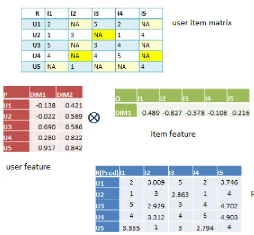
The RSVD model is scalable and works better in sparse dataset; however, the number of parameters in RSVD for both items and users are equal and are often large which increases the complexity of the model. With increasing data, the complexity of model increases, therefore main purpose of this paper is to develop a lesser complex model than RSVD, which is at least as accurate as RSVD.

(10)

factors of item and corresponding latent factor of user is approximated to known rating of user-item pair. Here, the number of latent factor of items varies depending on the dataset, but the number of latent factor of user is constant and equals to one. This model therefore, diminishes the number of latent factors to be trained in comparison to RSVD and hence is lesser complex than RSVD.

The equation of the above proposed model can be written mathematically:

�� ≈ ��∙ ∑ �� ∈�

Where, � are � latent features of item and �_� is a latent weight of the sum of all the latent features of an item rated by the user.

Like the RSVD model, an initial baseline estimate of every {user, item} pair is estimated using �_� = �_�+ � +  ; where �_� and � are observed deviation of user u and i from user average rating and item average rating and  is the global average of ratings of all the user, item rated. The base line estimate is added linearly with the above scheme, regularization parameter 1 is introduced to the new formed equation

which minimizes the sum of square of error between predicted and actual rating. The new scheme formed after incorporating baseline estimates and regularization is given by:

� �∗ �∗∑�,  �� −  − ��− � − ��∙ ∑ ∈�� + ‖��‖ _��+

‖∑ ��

∈� ‖ _��+ �� + � ) (7)

The equation can be solved by using SGD method as illustrated in RSVD. Since it is also a non-convex function as is RSVD model, it may not attain a global optimum value but can reach close to optimum value using SGD. In order to reach minima learning rate (1) is multiplied against the slope of descent at each iteration level. The

update of �_� and � for every user and every item can be done after each iteration in following manner.

� = �_� - �̂_�; (8)

�_� = �_� + 1 (2� *∑ _∈��-  �_� );

(9)

� = � + 1 (2e * �_� - � );

(10)

An important point with regard to this algorithm is stopping criteria, as soon as the sum of squares of the errors start stabilizing the algorithm is stopped. If the sum of square of the errors in last iteration approximately equals or has a very small prefixed difference () with the sum of square of the errors in previous iteration the model is thought to have learned and algorithm is stopped at that instance. The pseudo code for learning using stochastic gradient descent is described below:

Algorithm:

(11)

 : A matrix of rating, dimension N x M (user item rating matrix)

  : Set of known ratings in matrix

 _�_� : An initial vector of dimension N x 1 (User feature vector)

 _� : An initial matrix of dimension M x K (Movie feature matrix)

 _�_� : Bias of user �.

 _� : Bias of item �.

  : Average rating of all users

 K : Number of latent features to be trained

 _� : error between predicted and actual rating

Parameters:

 1 : learning rate

  : over fitting regularization parameter

 Steps : Number of iterations

Output: A matrix factorization approach to generate recommendation list

Method:

1) Initialize random values to matrix � and vectors, �_�, �_�and �

2) Fix value of K, 1 and .

3) do till error converges [ error(step-1) - error(step) < ɛ ]

error (step)= �_� −  − �_�− � − �_�∙ ∑ _∈�� + ‖�_�‖ + ‖� ‖ + ‖��‖ _�� + ‖∑ ∈��‖ _��

4) for each 

Compute � ≝ �_� −− �_�− � − �_�∙ ∑ _∈��

Update training parameters

�_� b_u+ 2e −  b_u

b b + 2e −  b

X_u X_u+ 2e ∑ _∈KZT −  P_u

Z Q + 2e X_u−  Z

5) endfor

6) end

7) return X_u, Z , b_uand b

(12)

Space complexity of the proposed model is lesser than RSVD as can be seen from the two models. In RSVD model the dimension of P_u and Q are N x K and M x K respectively, while the dimension of corresponding factors X_u and Z in proposed model are N x 1 and M x K respectively. This proves the compactness of the proposed model over RSVD model. Now, I will look into the accuracy of both the models in next section.

Figure 2: A schematic diagram for predicting ratings from sparse user-item rating matrix

Experimentation

Datasets

For the experimental evaluations of the proposed method, I make use of two different datasets. The first one is a publicly available Movie Lens dataset (ml-100k). The dataset consists of ratings of movies provided by users with corresponding user and movie IDs. There are 943 users and 1682 movies with 100000 ratings in the dataset. Had every user would have rated every movie total ratings available should have been 1586126 (i.e. 943×1682); however only 100000 ratings are available which means that not every user has rated every movie and dataset is very sparse (93.7%). This dataset resembles an actual scenario in E-commerce, where not every user explicitly or implicitly expresses preferences for every item.

(13)

review. The total number of users is 889,176 and total number of products is 253,059. In order to use this dataset for experimentation purpose I have randomly sub-sampled the dataset to include 6466 users and 25350 products with only users, items, ratings and timestamp intact in the data. The total number of ratings available in the sub-sampled dataset is 54996, which make the data sparser than ml-100 k dataset (99.67% sparsity).

In order to recommend items to users based on their past explicit behavior (ratings) for movies, I have assumed that ratings of 4 and 5 for a movie indicate preference for that movie, while ratings of 1, 2 and 3 for a movie suggest that user is not interested in that movie. Therefore, generating recommendation involves the task to predict ratings for unrated movies, and only those movies will be recommended to a user whose predicted rating lies in the range of 4 and 5.

3. EVALUATION MEASURES

1.1.2 _{Accuracy measures}

In order to evaluate accuracy, the Root Mean Square Error (RMSE) and Mean Absolute Error (MAE) are popular metrics in Recommender systems. Since, RMSE gives more weightage to larger values of errors while MAE gives equal weightage to all values of errors, RMSE is preferred over MAE while evaluating the performance of RS (Koren, 2009). RMSE is popular metrics in RS until very recently and many previous works have based their findings on this metrics, therefore this metrics has been used primarily to exhibit the performance of the proposed models and RSVD model on two datasets. For a test user item matrix ‘’ the predicted rating r̂_u for user-item pairs (u, i) for which true item rating r_u are known, the RMSE is given by

RMSE =√

|| ∑ u, ∈ r̂u − ru

MAE on the other hand is given by

MAE=

|| ∑u, ∈| r̂u − ru|

Cross validation

Cross validation is a well-established technique in machine learning algorithms that are used in evaluation of various algorithms. This technique ensures that the evaluation results are unbiased estimates and are not due to chance. For applying this technique, the dataset is split into disjoint k-folds; (k-1) folds are used as training set while the left out set is used for testing. The procedure is repeated k times so that each time a unique test set can be used for performance evaluation. The measures such as RMSE used for evaluation of RS models will be calculated k times and then averaged to get the resultant unbiased estimate of the performance measures.

k-Fold Cross-Validated Paired t Test

For testing, better of the two algorithms between RSVD and proposed model, I have performed cross-validated paired t test on both the datasets.

(14)

say by the test if the difference between the RMSE zero or not but I cannot establish the better of the two algorithm. Therefore, I have to modify the null hypothesis. The null hypothesis to establish the better of the two algorithms can be modified to; that the RMSE obtained for validation sets by RSVD is less than RMSE obtained for validation sets by the proposed model. By using paired t test I can statistically prove the better of the two algorithms for the both the datasets (Alpaydin, 2004).

4. OBSERVATIONS AND RESULT

For the proposed model latent feature value of K is varied from 5 to 30 in step size of 5, and I record the RMSE values in table 2. To compare both the models on MovieLens dataset (ml-100k),  (regularizing parameter) and  (learning rate) are taken as 0.01 and 0.01 respectively that were found using cross-validation. By comparing both the models I found that RMSE reaches its minima at K= 5 for both RSVD and proposed model, and the minima of both the model happens for the proposed model at K= 5. To establish that the proposed model is better than RSVD for ml-100k dataset I have used k-fold cross-validated paired t test at 0.05 levels of significance. The null hypothesis that the RMSE obtained for validation sets by RSVD is less than RMSE obtained for validation sets by the proposed model is rejected as the p-value is found to be 0.9995, and the alternative hypothesis is accepted.

I have also used amazon dataset and followed the above procedure to establish the claim of better RMSE from proposed model than RSVD. In order to compare both the models on amazon dataset,  (regularizing parameter) and  (learning rate) are taken as 0.001 and 0.1 respectively. Table 3 reveals the RMSE of both the algorithms at various Kvalues. By comparing both the models I found that RMSE reaches its minima at K= 5 for RSVD and at K= 20 for proposed model, the overall minima of both the models occurs for the proposed model at K= 20. I have used k-fold cross-validated paired t test at 0.05 levels of significance for finding the better of the two models. The null hypothesis that the RMSE obtained for validation sets by RSVD is less than RMSE obtained for validation sets by the proposed model is rejected as the p-value is found to be 1, and the alternative hypothesis is accepted.

d 5 10 15 20 25 30 MEAN SD

RSVD RMSE 0.948 0.949 0.948 0.956 0.959 0.967 0.955 0.007

Proposed Model RMSE 0.936 0.939 0.943 0.95 0.959 0.977 0.951 0.014

Table2: comparison of RMSE on Ml-100k dataset

d 5 10 15 20 25 30 MEA

N

SD

(15)

JISTEM, Brazil Vol. 13, No. 3, Set/Dez., 2016 pp. 497- 514 www.jistem.fea.usp.br Propose

d Model

RMSE 1.0342 1.0298 1.0291 1.0278 1.0453 1.0567 1.0371 0.0115

Table 3: comparison of RMSE on amazon dataset

The results of the proposed model are reported on two different datasets, viz., Ml-100k and amazon dataset. RMSE values on both these datasets are significantly lower or as accurate when compared with state-of-the art RSVD model. It is also to be noted that the complexity of the proposed model is lower than RSVD model, which signifies its deployment in practical scenarios where there are large sparse data to be handled efficiently.

5. CONCLUSION

The data on e-commerce platform is growing at increasing velocity with every passing day, so it is a growing challenge for researchers and industry practitioners to build recommenders that are faster to use and accurate in recommendation. The proposed model in this paper has shown through empirical evaluation that it is as accurate as RSVD if not better in terms of accuracy as well as the space complexity is much lesser than RSVD.

The proposed model has also been successful in handling sparsity, which is one of the main reasons of using RSVD in sparse dataset. I can see from the empirical evaluations that the proposed model fares better than RSVD model in terms of accuracy when data is sparser. This observation is true in case of this dataset and drawing generalization for similar sparser dataset may be a far-fetched conclusion. This observation can be checked thoroughly in other datasets with more or less sparsity. One of the limitations of the models is that the rating prediction can go out of bounds which is also one of the limitations of RSVD model. The out of bound prediction can reduce the performance of the model, if not tackled either by clipping or by some other method as described for RSVD method.

Further, the proposed model can be extended to learn parameters so that the recommendations of good items can be improved. This can be achieved by modelling the proposed scheme so that it takes care of precision and recall of the recommender system. To improve the accuracy of proposed model I can also use gradient boosting of the proposed model which a kind of ensemble technique by varying parameters of the proposed model.

REFERENCES

Adolphs, C., & Winkelmann, A. (2010). Personalization Research in E-Commerce–A State of the Art Review (2000-2008). Journal of Electronic Commerce Research, 11(4), 326–341.

Agarwal, D., & Chen, B.-C. (2009). Regression-based latent factor models. In

(16)

JISTEM, Brazil Vol. 13, No. 3, Set/Dez., 2016 pp. 497- 514 www.jistem.fea.usp.br discovery and data mining (pp. 19–28). ACM.

Ahmed, A., Kanagal, B., Pandey, S., Josifovski, V., Pueyo, L. G., & Yuan, J. (2013). Latent factor models with additive and hierarchically-smoothed user preferences.

Proceedings of the Sixth ACM International Conference on Web Search and Data Mining - WSDM ’13. https://doi.org/10.1145/2433396.2433445

Alpaydin, E. (2004). Introduction to Machine Learning (Adaptive Computation and Machine Learning). The MIT Press.

Bauer, J., & Nanopoulos, A. (2014). Recommender systems based on quantitative implicit customer feedback. Decision Support Systems, 68, 77–88.

Billsus, D., & Pazzani, M. J. (1998). Learning Collaborative Information Filters. In

Proceedings of the Fifteenth International Conference on Machine Learning (pp. 46– 54). San Francisco, CA, USA: Morgan Kaufmann Publishers Inc. Retrieved from http://dl.acm.org/citation.cfm?id=645527.657311

Blei, D. M., Ng, A. Y., & Jordan, M. I. (2003). Latent Dirichlet Allocation. Journal of Machine Learning Research, 3, 993–1022. Retrieved from http://dl.acm.org/citation.cfm?id=944919.944937

Bobadilla, J., Ortega, F., Hernando, A., & Gutiérrez, A. (2013). Recommender systems

survey. Knowledge-Based Systems, 46, 109–132.

https://doi.org/10.1016/j.knosys.2013.03.012

Breese, J. S., Heckerman, D., & Kadie, C. (1998). Empirical Analysis of Predictive Algorithms for Collaborative Filtering. In Proceedings of the Fourteenth Conference on Uncertainty in Artificial Intelligence (pp. 43–52). San Francisco, CA, USA: Morgan

Kaufmann Publishers Inc. Retrieved from

http://dl.acm.org/citation.cfm?id=2074094.2074100

Canny, J. (2002). Collaborative Filtering with Privacy via Factor Analysis. In

Proceedings of the 25th Annual International ACM SIGIR Conference on Research and Development in Information Retrieval (pp. 238–245). New York, NY, USA: ACM. https://doi.org/10.1145/564376.564419

Cheung, K. W., Kwok, J. T., Law, M. H., & Tsui, K. C. (2003). Mining customer product ratings for personalized marketing. Decision Support Systems, 35(2), 231–243. https://doi.org/10.1016/S0167-9236(02)00108-2

Chung, C. Y., Hsu, P. Y., & Huang, S. H. (2013). Bp: A novel approach to filter out malicious rating profiles from recommender systems. Decision Support Systems, 55(1), 314–325. https://doi.org/10.1016/j.dss.2013.01.020

Cremonesi, P., Koren, Y., & Turrin, R. (2010). Performance of recommender algorithms on top-n recommendation tasks. In Proceedings of the fourth ACM conference on Recommender systems - RecSys ’10 (p. 39). https://doi.org/10.1145/1864708.1864721

Ekstrand, M. D. (2010). Collaborative Filtering Recommender Systems. Foundations and Trends® in Human–Computer Interaction, 4(2), 81–173. https://doi.org/10.1561/1100000009

Gan, M., & Jiang, R. (2013). Improving accuracy and diversity of personalized recommendation through power law adjustments of user similarities. Decision Support Systems, 55(3), 811–821. https://doi.org/10.1016/j.dss.2013.03.006

(17)

https://doi.org/10.1023/A:1011419012209

Ho, Y., Kyeong, J., & Hie, S. (2002). A personalized recommender system based on web usage mining and decision tree induction, 23, 329–342.

Hofmann, T. (2004). Latent Semantic Models for Collaborative Filtering. ACM Transaction on Information System, 22(1), 89–115. https://doi.org/10.1145/963770.963774

Jawaheer, G., Weller, P., & Kostkova, P. (2014). Modeling User Preferences in Recommender Systems: A Classification Framework for Explicit and Implicit User Feedback. ACM Transactions on Interactive Intelligent Systems, 4(2), 8:1--8:26. https://doi.org/10.1145/2512208

Jin, R., & Si, L. (2004). A bayesian approach toward active learning for collaborative filtering. Proceedings of the 20th Conference on Uncertainty in Artificial Intelligence, 278–285. Retrieved from http://dl.acm.org/citation.cfm?id=1036877

Kim, Y. S., Yum, B.-J., Song, J., & Kim, S. M. (2005). Development of a recommender system based on navigational and behavioral patterns of customers in e-commerce sites.

Expert Systems with Applications, 28(2), 381–393.

Konstan, J. A., & Riedl, J. (2012). Recommender systems: From algorithms to user experience. User Modelling and User-Adapted Interaction, 22(1–2), 101–123. https://doi.org/10.1007/s11257-011-9112-x

Koren, Y. (2008). Factorization meets the neighborhood: a multifaceted collaborative filtering model. In Proceedings of the 14th ACM SIGKDD international conference on Knowledge discovery and data mining (pp. 426–434). ACM.

Koren, Y. (2009). The bellkor solution to the netflix grand prize. Netflix Prize Documentation, (August), 1–10. https://doi.org/10.1.1.162.2118

Koren, Y., & Bell, R. (2011). Advances in Collaborative Filtering. In Recommender Systems Handbook (pp. 145–186). https://doi.org/10.1007/978-0-387-85820-3

Koren, Y., & Sill, J. (2011). OrdRec : An Ordinal Model for Predicting Personalized Item Rating Distributions. In Recsys ’11.

Kumar, R., Raghavan, P., Rajagopalan, S., & Tomkins, A. (2001). Recommendation Systems : A Probabilistic Analysis, 61, 42–61.

Ma, H., Zhou, D., Liu, C., Lyu, M. R., & King, I. (2011). Recommender Systems with Social Regularization. In Proceedings of the Fourth ACM International Conference on Web Search and Data Mining (pp. 287–296). New York, NY, USA: ACM. https://doi.org/10.1145/1935826.1935877

Mishra, R., Kumar, P., & Bhasker, B. (2015). A web recommendation system considering sequential information. Decision Support Systems, 75, 1–10. https://doi.org/10.1016/j.dss.2015.04.004

Parambath, S. A. P. (2013). Matrix Factorization Methods for Recommender Systems, 44. Retrieved from http://www.diva-portal.org/smash/record.jsf?pid=diva2:633561 Paterek, A. (2007). Improving regularized singular value decomposition for collaborative filtering. In Proc. KDD Cup Workshop at SIGKDD’07, 13th ACM Int.

Conf. on Knowledge Discovery and Data Mining (pp. 39–42). Retrieved from http://serv1.ist.psu.edu:8080/viewdoc/summary;jsessionid=CBC0A80E61E800DE5185 20F9469B2FD1?doi=10.1.1.96.7652

(18)

Rennie, J. D. M., & Srebro, N. (2005). Fast Maximum Margin Matrix Factorization for Collaborative Prediction. In Proceedings of the 22Nd International Conference on Machine Learning (pp. 713–719). New York, NY, USA: ACM. https://doi.org/10.1145/1102351.1102441

Russell, S., & Yoon, V. (2008). Applications of Wavelet Data Reduction in a Recommender System. Expert System with Applications, 34(4), 2316–2325. https://doi.org/10.1016/j.eswa.2007.03.009

Salakhutdinov, R., & Mnih, A. (2008). Bayesian probabilistic matrix factorization using Markov chain Monte Carlo. In Proceedings of the 25th international conference on Machine learning (pp. 880–887).

Salakhutdinov, R., Mnih, A., & Hinton, G. (2007). Restricted Boltzmann machines for collaborative filtering. In Proceedings of the 24th international conference on Machine learning (pp. 791–798). ACM.

Sarwar, B., Karypis, G., Konstan, J., & Riedl, J. (2000). Application of dimensionality reduction in recommender system-a case study. In ACM WebKDD 2000 Workshop. Sarwar, B., Karypis, G., Konstan, J., & Riedl, J. (2002). Incremental singular value decomposition algorithms for highly scalable recommender systems. Fifth International Conference on Computer and Information Science, 27–28.

Sarwar, B. M., Karypis, G., Konstan, J. a, & Riedl, J. T. (2000). Application of dimensionality reduction in recommender systems: a case study. In ACM WebKDD

Workshop, 67, 12. Retrieved from

http://citeseerx.ist.psu.edu/viewdoc/summary?doi=10.1.1.38.744

Shardanand, U., & Maes, P. (1995). Social information filtering. Proceedings of the SIGCHI Conference on Human Factors in Computing Systems - CHI ’95, 210–217. https://doi.org/10.1145/223904.223931

Su, X., & Khoshgoftaar, T. M. (2009). A Survey of Collaborative Filtering Techniques.

Advances in Artificial Intelligence, 2009, 1–19. https://doi.org/10.1155/2009/421425 Vahidov, R., & Ji, F. (2005). A diversity-based method for infrequent purchase decision support in e-commerce, 4, 143–158. https://doi.org/10.1016/j.elerap.2004.09.001

Vozalis, M., & Margaritis, K. (2007). Using SVD and demographic data for the enhancement of generalized Collaborative Filtering. Information Sciences, 177(15), 3017–3037. https://doi.org/10.1016/j.ins.2007.02.036

Yang, X., Guo, Y., Liu, Y., & Steck, H. (2014). A survey of collaborative filtering based social recommender systems. Computer Communications, 41, 1–10. https://doi.org/10.1016/j.comcom.2013.06.009

Yu, K., Zhu, S., Lafferty, J., & Gong, Y. (2009). Fast Nonparametric Matrix Factorization for Large-scale Collaborative Filtering. In Proceedings of the 32Nd International ACM SIGIR Conference on Research and Development in Information

Retrieval (pp. 211–218). New York, NY, USA: ACM.

https://doi.org/10.1145/1571941.1571979

Zhang, X., Edwards, J., & Harding, J. (2007). Personalised online sales using web usage data mining, 58, 772–782. https://doi.org/10.1016/j.compind.2007.02.004