Saturation in High-energy QCD
Gr´egory Soyez∗
SPhT, CEA/Saclay, Orme des Merisiers, B ˆat 774, F-91191 Gif-sur-Yvette cedex, France
Received on 17 May, 2006
In these proceedings, I shall review the basic concepts of perturbative QCD in its high-energy limit, empha-sising the approach to the unitarity limit, usually referred to assaturation. I shall explain the basic framework showing the need for saturation, first, from a simple picture of the high-energy behaviour, then, giving a short derivation of the equation driving this evolution. In the second part, I shall exhibit an analogy with statistical physics and show how this allows to derivegeometric scalingin QCD with saturation. I shall finally consider the effects of gluon-number fluctuations on this picture.
Keywords: High-energy QCD; Saturation; Geometric scaling
I. INTRODUCTION
The quest for the high-energy behaviour of perturbative QCD started thirty years ago, soon after QCD was proposed as the fundamental theory of strong interactions. To grasp this problem, it has been realised that saturation effects were to be considered in order to satisfy unitarity constraints. Through-out these proceedings, I shall summarised the present status of our understanding of this limit, which basically means finding an equation giving the evolution of amplitudes towards high energy and finding the properties of its solutions.
Non
p
erturbativ
e
log(
Q
2)
log
(1
/x
)
DGLAP
BFKL
Q
=
Q
s(
Y
)
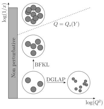
FIG. 1: Picture of the proton in DIS
In order to motivate the physical picture we want to repro-duce, let us consider the problem of Deep Inelastic Scattering (DIS)i.e. γ∗p→X collisions. This process depends on two
∗On leave from the fundamental theoretical physics group of the University
of Li`ege.
kinematical variables: the virtualityQ2 of the photon, mea-suring the resolution at which the photon scans the proton, and the Bjorken x, given by the fraction of the proton mo-mentum carried by the parton struck by the virtual photon in a frame where the proton is moving fast. This last variable is related to the centre-of-mass energys=Q2/x, meaning that the high-energy limit corresponds to the small-xlimit. For practical purposes, we introduce therapiditydefined through Y=log(1/x).
In Figure 1, we have represented the typical configuration of the proton in different domains of this phase space. We start with a proton at lowQ2and low energy, represented as three partons (bottom-left part of the picture). If we increase the virtuality of the photon, we are able to resolve its partons into smaller ones. This type of evolution is described in QCD by the Dokshitzer-Gribov-Lipatov-Altarelli-Parisi (DGLAP) equation [1]. In that limit, the number of partons rises log-arithmically while their typical size decreases like 1/Q2 so that the proton becomes more and more dilute. In what fol-lows, we shall be interested in the other type of evolution, namely the evolution towards smaller values ofxfor constant Q2. If one boosts the proton, what typically happens is that we create new partons of a size comparable to the parents’ ones. Obviously, during this evolution, known as the Balitsky-Fadin-Kuraev-Lipatov (BFKL) evolution [2], the proton tends to the black-disc limit for which partons start to overlap. At that level, they start to interact among themselves and unitar-ity corrections are to be considered [3]. This blackening of the proton is called saturation and is what we shall describe from perturbative QCD in these proceedings.
satu-ration.
II. EVOLUTION TOWARDS HIGH ENERGY
Let us start with a fast-moving quark of momentump. This quark emits Bremsstrahlung gluons characterised by their transverse momentumk2
⊥and their longitudinal momentum kz=xp. The probability for emitting such a gluon is
dP∼αs dx
x dk2⊥
k2⊥ .
When we consider large transverse momentum (highQ2 in DIS), the collinear divergencesdk2⊥/k2⊥need to be resummed and this gives rise to a renormalisation group equation known as the DGLAP equation. Throughout this proceedings, we shall instead consider the limit of high energy, in which, we are sensitive to the gluons of small longitudinal momentum x≪1. This leaves a large phase-space to have successive gluon emissions satisfying 1≫x1≫ ··· ≫ xn≫x which
gives a contribution of order
αns
1
x dx1
x1
. . .
1
xn−1 dxn
xn
= 1
n!α
n
log(1/x)n.
Even when the couplingαsis small enough to ensure
applica-bility of perturbation theory, for small values ofx i.e. high-energy,αslog(1/x)∼1 and all these contributions have to be
resummed.
≡
FIG. 2: Gluon emission in the dipole picture
In order to simplify the discussion, let us consider the case of a large number of colours. In that limit, a gluon of trans-verse coordinatezcan be considered as a quark-antiquark pair at pointz. In this framework, it is convenient to consider the evolution of a colourless quark-antiquark dipole [14]. Indeed, at high-energy, all possible gluon emissions from one dipole are tantamount to this dipole splitting into two child dipoles as depicted in figure 2. We can thus forget about gluons them-selves and talk only in term of dipoles.
Let us denotes byTxythe scattering amplitude1for a di-pole made of a quark at transverse coordinatexand an anti-quark aty. Getting the evolution ofTfrom the dipole pic-ture is pretty straightforward. Indeed, if one boosts the dipole
(x,y)from a rapidityY to a rapidityY+δY, this dipole shall split into two dipoles(x,z)and(z,y). Each of those dipoles
1The notation
·denotes the average over all possible realisations of the target colour field. It can be understood as the expectation value for the
T-matrix operator over the target wavefunction.
≡
FIG. 3: Multiple scattering between a target and a projectile made of two dipoles. This can be interpreted as pomeron merging in the target.
can interact with the target which leads to the following evo-lution equation2forT
∂YTxy= ¯
α
2π
z
M
xyz(Txz+Tzy − Txy) (1)with ¯α=αsNc/πand
M
xyz =x
−z (x−z)2−
y−z (y−z)2
2
= (x−y)
2
(x−z)2(z−y)2
is the probability density for dipole splitting3. Equation (1) is the BFKL equation, derived in the mid-seventies [2] by Balit-sky, Fadin, Kuraev and Lipatov.
This equation being linear, one expects its solution to grow exponentially. To be more explicit, if one neglects impact-parameter dependence, i.e. assumes that Txy =
T(r=|x−y|), the solution of (1) is
T(r)=
dγ
2iπT0(γ)e
χ(γ)Y−γlog(r2
0/r2), (2)
whereχ(γ) =2ψ(1)−ψ(γ)−ψ(1−γ) and T0(γ) describes the initial condition. For a fixed dipole size, one finds the high energy behaviour in the saddle point approximation
T(r) ∼exp
ωPY−
log2(r20/r)
2χ′′(1/2)α¯Y
,
with ωP=4πlog(2)α¯ being the BFKL pomeron intercept.
This expression suffers from two major problems: first, even if one start with an initial condition peaked around a small value ofr, when rapidity increases, the amplitude starts to diffuse to the large dipole sizesi.e.to the non-perturbative domain. Sec-ond, the solution of the BFKL equation grows exponentially with rapidity. It hence violates the unitarity constraintT ≤1 obtained from first principles.
This unitarity problem is precisely the point where we meet the requirement to take into account multiple interactions. The
2The last term, coming with a minus sign, corresponds to virtual corrections 3The first line shows explicitly the two contributions coming from emission
most straightforward way to see this is to come back to the splitting of a dipole(x,y)into(x,z)and(z,y). When the tar-get becomes dense enough, both dipoles can scatter on it. We thus have to take into account this contribution, represented in figure 3. This leads to a quadratic suppression term in the evolution equation which becomes
∂YTxy= ¯
α
2π
z
M
xyzTxz+Tzy − Txy −
Txz2;zy . (3) The first thing to remark is that this new term is of the same order as the previous ones whenT2∼T or, equivalently, when T ∼1. It is thus, as expected, a mandatory contribution near the unitarity limit. However, equation (3) involves a new ob-ject, namely
Txz2;zy
which probes correlations inside of the target. In a general framework, one should then write down an equation forT2, which will involveT2through BFKL-like contributions and
T3
from unitarity requirements. This ends up with a complete hierarchy, giving the evolution for each
Tk, known as the (large-Nc) Balitsky hierarchy [4].
If the target is sufficiently large and homogeneous, one can simply assumeTxz2;zy=TxzTzy, ending up with a closed equation forT
∂YTxy= ¯
α
2π
z
M
xyz(Txz+Tzy − Txy − TxzTzy).(4) This last expression is the Balitsky-Kovchegov (BK) equa-tion [4, 6], which is the most simple equaequa-tion one can obtain from perturbative QCD by including both the BFKL contribu-tions at high-energy and the correccontribu-tions from unitarity. It is easy to check thatT=0 is an unstable fix point of the BK equation, whileT=1 is a stable fix point, ensuring unitar-ity is satisfied. In general, unitarunitar-ity effects cut the increase of the amplitude for scales smaller than a typical scale, called the saturation momentum, increasing with rapidity. In particular, it solves the problem of diffusion to the infrared obtained with linear BFKL equation. We shall come back with more details to the study of the solution of the BK equation for the next section.
If one wants to study those effects beyond the large-Nc
approximation, one better used the colour-glass-condensate (CGC) formalism. This is an effective theory in which one consider the radiation of soft gluons in a strong background field which introduces the nonlinear effects requested at satu-ration. At a given rapidity, the target is considered as a random colour sourceρa(x)and radiates a field according to the QCD
Yang-Mills equations. We then study the rapidity evolution of the functionalWY[ρ]giving the probability to find a sourceρ
at rapidityY. This functional allow to compute the average value of an operator using
O
Y =
D
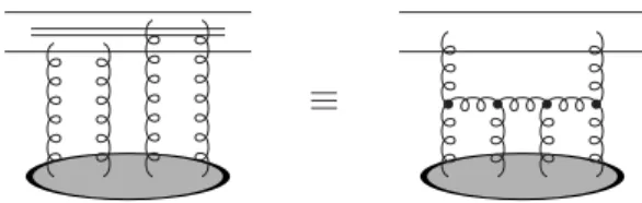
[ρ]WY[ρ]O[ρ]. (5)We thus need to find the evolution ofW[ρ]. One step of evolution is represented diagrammatically in figure 4. As for the BFKL equation, one soft gluon is radiated (yielding a
αslog(1/x)factor). The difference comes from the fact that
W
Y[
ρ
]
δY
W
Y[
ρ
]
≡
W
Y+δY[
ρ
]
FIG. 4: One step of JIMWLK evolution: the emitted soft gluon prop-agating in the string target field is used to redefine the probability W[ρ]at rapidityY+δY. The case of two gluons only corresponds to BFKL.
when the target is sufficiently dense, one has to dress the prop-agator of this soft gluon with the field created by the target. These emissions are then reabsorbed inside the probability W[ρ]in order to define it at rapidityY+δY. Each background gluon insertion gives a factorgα withg the QCD coupling andαthe A+ colour field of the target. Including these ef-fects becomes mandatory when the field is of order 1/g. The amplitude is defined through
Txy=1− 1 Nc
trWx†Wy
, (6)
whereWxis the Wilson line operator
Wx=Pexp
ig
∞
−∞
dx−α(x−,x)
,
which means that in the leading order,Txy∝g2(αx−αy)2. This shows that the strong fieldα∼1/gcorresponds toT∼1 and thus to saturation corrections. A careful treatment of the diagrams in figure 4 leads to the JIMWLK equation [5]
∂YWY[ρ] =
D
[ρ] δδρa
x
χab
xy
δ δρb
y
WY[ρ], (7)
with the kernelχcomputable in perturbative QCD.
This functional integro-differential equation gives the ra-pidity evolution ofW[ρ]. Using relations like (5) or (6), one can obtain the evolution of the scattering amplitudes. The resulting equations are equivalent to the Balitsky hierarchy [4]. These equations going beyond largeNc, they involves
non-dipolar operators. For example, the equation for two dipoles depends on a sextupole operator (build out of six Wil-son lines). The formalism beyond largeNcbeing rather tricky,
in what follows we shall stick to the BK equation, which is sufficient to grasp the basic concepts of saturation.
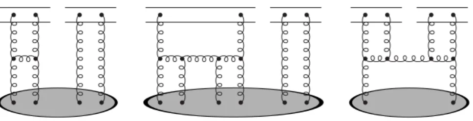
Very recently, it has been realised that the question of the high-energy limit of QCD, even at the leading logarithmic ac-curacy, is not fully described by the Balitsky hierarchy. To see this more precisely, let us consider in more details the evolution equation for
T2
. It corresponds to the scatter-ing of two dipoles off a target and the diagrams contributscatter-ing to one step of rapidity evolution are shown in figure 5. The first graph on the left of this figure is simply the BFKL-ladder contribution for which∂Y
T2∝
FIG. 5: Diagrams contributing to the evolution of
T2
. They correspond, from left to right, to BFKL ladders, saturation corrections and fluctuations effects.
It accounts for unitarity corrections and gives a contribution
∂Y
T2∝
T3. If those two graphs were the only relevant ones in the evolution, one would obtain the (large-Nc)
Bal-itsky equation. Nonetheless, it has been argued that a third contribution, represented by the rightmost diagram of figure 5, has to be included. This graph describes multiple scattering off the projectile or, equivalently, gluon-number fluctuations inside the target. After the pomeron-merging term, contribut-ing to saturation, one thus now also includes the pomeron-splitting contribution, which gives rise to a new term in the evolution equation ∂YT2∝T. For large-Nc and at the
two-gluon-exchange level, this new term has been computed [12] and leads to
∂YTx21y1;x2y2
fluct= 1 2
¯
α
2π αs
2π 2
(8)
uvz
M
uvzA
0(x1y1|uz)A
0(x2y2|zv)∇2u∇2vTuv+ (1↔2), with
A
0being the dipole-dipole amplitude at thetwo-gluon-exchange level
A
0(xy|uv) =18log 2
(x−u)2(y−v)2
(x−v)2(y−u)2
.
This object naturally comes out when we relate the scattering amplitude with the dipole densityn:
Txy=α2s
uv
A
0(xy|uv)nuv. (9)This relation can be inverted to obtainnxy=α−s2∇2x∇2yTxy. The correction (8) becomes of the same order as the BFKL contribution when T2∼α2
sT, or T ∼α2s, i.e. in the dilute
regime where, as expected, fluctuations should lead to im-portant effects. Although this may at first sight seems irrel-evant for the physics of saturation, one has to realise that, due to colour transparency, the amplitude becomes arbitrar-ily small for small dipole size, hence, even for dense ob-jects, there is always some region of the phase-space where the system is dilute and its evolution governed by fluctua-tion effects. Once the system has evolved through a fluctu-ation, it grows, from BFKL evolution, like two pomerons, i.e. T ∼α2
sexp(2ωPY). This has to be compared with the
one-pomeron exchangeT ∼exp(ωPY). We see that at very
large energiesY ≥ω−P1log(1/α2
s), BFKL evolution
compen-sates the extra factor ofα2
s coming from the initial fluctuation.
We shall see more precisely in the last section that those fluc-tuation effects in the dilute tail have important consequence on the saturation physics.
Finally, let us conclude this section by quoting that the equation (8), including linear, saturation and fluctuation ef-fects is the most complete equation known in perturbative high-energy QCD so far. Its extension beyond the large-Nc
approximation is still a challenging problem.
III. PROPERTIES OF THE SCATTERING AMPLITUDES
In this section, we shall sketch out the main properties of the solutions of the evolution equations towards high energy. As we shall explain in detail in the next lines the major source of information comes from the analogy between the BK equation and the Fisher-Kolmogorov-Petrovsky-Piscounov (F-KPP) equation which is very well studied in statistical physics. This section shall be devoted to derive this anal-ogy and its consequences in the case of the BK equation. We leave the discussion concerning the effect of fluctuations for the next section.
So, let us start with the BK equation (4). We shall first re-strict ourselves to the impact-parameter-independent version of the equation, for which one can easily go to momentum space by using4
˜
T(k) = 1
2π
d2r
r2 e
ik.rT(r) = ∞ 0
dr
r J0(kr)T(r),
and where the equation becomes
∂YT˜(k) =αχ(¯ −∂L)T˜(k)−α¯T˜2(k), (10)
withL=log(k2/k20),k0being a soft reference scale.
In order to simplify the problem, we shall work in the sad-dle point approximation (often referred to as thediffusive ap-proximation) and expand the BFKL kernel to second order aroundγ=1/2, transforming the complicated differential op-erator in equation (10) into a second-order opop-erator
χ(−∂L)T˜(k)≈χ(12) +12χ′′(12) (∂L+12)
2.
4In this section, we omit the·quotations as they do not play any role in
log(k2)
T
40 35 30 25 20 15 10 5 0 -5 10
1
0.1
0.01
0.001
1e-04
1e-05
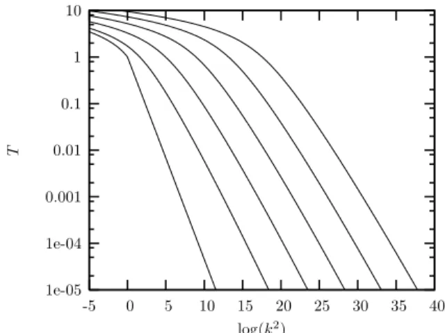
FIG. 6: Numerical simulation of the rapidity-evolution of the BK equation. We start atY=0 from the leftmost amplitude and evolve to higherY using (10). Amplitude is shown forY =5,10,15,20,25 and clearly exhibits a travelling-wave pattern.
N= 0.5 N= 0.1 N= 0.05 N= 0.01
Y 1 Y
lo
g
Qs
2(
Y
)
Qs
2(0)
50 45 40 35 30 25 20 15 10 1.4
1.2
1
0.8
0.6
0.4
0.2
0
FIG. 7: Rapidity evolution of the saturation scale extracted from fig-ure 6. More precisely, the speed of the wave,i.e.the exponent of the saturation scale, is plotted. It goes to a constant as it should.
Up to a linear change of variable switching fromY andLto timet=α¯Y and spacex=L+cst.Y and a renormalisation of the amplitudeT →u=cst.T, the BK equation in the saddle point approximation becomes
∂tu(x,t) =∂2xu(x,t) +u(x,t)−u2(x,t).
This equation is nothing but the F-KPP equation studied in statistical physics since forty years and applying to many problem. It describes reaction diffusion processes in the mean-field approximation where one can have creation and annihilation of particles locally and diffusion to neighbouring sitee.g.the density of population in the centre of Rio.
One knows that the F-KPP equation admits travelling waves as asymptotic solutionsi.e. there exists a critical velocityvc
and a critical slopeγc, determined only from the knowledge
of the linear kernel of the F-KPP equation∂2
x+1, such that
(see figure 6 for a pictorial representation coming from the BK equation which we shall explain a bit later)
u(x,t)−→t→∞u(x−vct) x≫vct
≈ e−γc(x−vct)log(x−v
ct).
Although working in the diffusive approximation makes the discussion easier due to the direct analogy with the F-KPP equation, this assumption is not required. Indeed, for an equa-tion with a more complicated kernel (than∂2
x+1), one can
prove the existence of travelling waves provided the three fol-lowing conditions are satisfied
1. the amplitude has 0 as unstable fix point and 1 as stable fix point,
2. the initial condition decreases faster than exp(−γcL)at
largeL(see below for the general definition ofγc),
3. the equation obtained by neglecting the nonlinear terms admits superposition of waves as solution.
Then, travelling waves are formed during evolution with the critical parameters obtained, from the linear kernel only, through the relation
vc=χ′(γc) = χ(γc)
γc
.
One can show that this corresponds to the selection of the wave with the minimal speed χ(γ)/γ and the point where group and phase velocities are equal.
In the case of the BK equation, the first condition is satisfied due to BFKL growth and saturation, the second comes from colour transparency (T∝1/k2=exp(−L)) and the last one is equivalent to the solution (2) (withr/r0replaced byk0/k) of the BFKL equation obtained by neglecting nonlinear terms in (10).
The critical parameters (for the complete BFKL kerneli.e. for (10)), are found to beγc≈0.6275 andvc≈4.8836 ¯α.
Writ-ten in terms of the QCD variablesY andk2, one can then write the asymptotic solution for the impact-parameter-independent BK equation under the form
T(k;Y)Y→=∞T
k2
Q2
s(Y)
k≫Qs
=
k2
Q2
s(Y)
−γc
log
k2
Q2
s(Y)
,
(11) with the saturation scale given by
Q2s(Y)Y→=∞k20exp
vcY−
3 2γc
log(Y)
. (12)
The formation of a travelling-wave pattern when energy in-creases can easily be seen on numerical simulations of the BK equation. As displayed in figure 6, if one start with a steep enough initial condition (leftmost curve), the amplitude in-creases with energy and a wave moving into the dilute domain gets formed. From that simulation, one can extract the satura-tion scale by solvingT(Q2s,Y) =Nat each values ofY and for a fixed thresholdN. In figure 7, we have plotted log(Q2s)/Y which goes to a constant value as it is expected from (12).
from the BK equation is one of the most important indication for the experimental observation of saturation. The saturation scale obtained from the structure function data is of the order of 1 GeV forx∼10−5. This means that high-energy QCD can indeed be studied from perturbation theory.
Up to now, we have only discussed the impact-parameter independent BK equation. We might therefore ask whether or not these arguments extend to the full equation including all phase-space degrees of freedom. A dipole of transverse coordinates(x,y)is then represented through its sizer=x−y
and impact parameterb= (x+y)/2. The problem is then that dipole splitting is non-local in impact parameter. This means that the BK equation couples different values ofband we can not apply directly the previous arguments for each value ofb. Again, the solution consists in moving to momentum space and replace the impact parameter by momentum transferq
˜
T(k,q) =
d2x d2y eik.xei(q−k).yT(x,y)
(x−y)2.
The BK equation then takes a form [15] for which the BFKL kernel is local inq
∂YT˜(k,q) (13)
= α¯ π
d2k′
(k−k′)2
˜
T(k′,q)−1
4
k2 k′2+
(q−k)2
(q−k′)2
˜ T(k,q)
− α¯
2π
d2k′T˜(k,k′)T˜(k−k′,q−k′).
We can now proceed with this equation in a similar way as for the the impact-parameter-independent case. The existence of travelling waves required the three conditions stated previ-ously to be satisfied. The two first ones are trivially satisfied5. For the third condition to be valid, we need to find solutions of the linear part of (13), i.e. the complete BFKL equation, which can be expressed as a superposition of waves. This is merely technical as it consists in a careful treatment of the so-lutions of the BFKL equation [16] in its full glory, so I shall directly jump to the results. We can show [17] that when the dipole momentumkis much larger than the momentum trans-ferqand the typical scale of the targetk0, the solutions of the BFKL equation are a superposition of waves and therefore, we obtain travelling waves for the full BK equation. More precisely, the high-energy behaviour of the amplitude takes the form
˜
T(k,q;Y) Y→=∞ T
k2
Q2
s(q;Y)
k≫Qs
=
k2
Q2
s(q;Y)
−γc
log
k2
Q2
s(q;Y)
.
This expression is exactly the same as for the previous case except that the saturation scale now depends on momentum
5Indeed, we have saturation and BFKL growth ensuring the first condition
and colour transparency still apply for the second one.
transfer
Q2s(q;Y)Y→=∞Λ2 exp
vcY−
3 2γc
log(Y)
with
Λ2=
k20 ifk0≫q q2 ifq≫k0
.
It is interesting to notice that the critical slopeγcad speedvc,
obtained from the BFKL kernel only, are the same as for the impact-parameter-independent case.
The important point at this stage is that this studypredicts geometric scaling at non-zero momentum transfer. Experi-mental measurements of the DVCS cross-sections or diffrac-tiveρ-meson production are good candidates and can provide more evidence for saturation.
IV. HIGH-ENERGY QCD WITH FLUCTUATIONS
Let us now consider the effect of adding the fluctuation con-tribution (8). This new term, added to the full Balitsky archy, turns a simple non-linear equation into a infinite hier-archy with a complicated transverse-plane dependence6. We can however simplify the equation to a tractable problem by performing a local-fluctuations approximation. This amounts to simplify the dipole-dipole scattering amplitude
A
0used torelate the dipole density n with the scattering amplitudeT. We assume that two dipoles interact if they are of the same size and if their centre-of-mass are sufficiently close to allow for an overlap of the two dipoles. Within this approximation equation (9) is replaced
Txy=κα2s |x−y|
4
nxy,
whereκis an unknown fudge factor of order 1.
Once this is done, the remaining steps are no particularly illuminating: one Fourier-transform the dipole sizer=|x−y|
into momentumkand perform a coarse-graining approxima-tion to get rid of the impact-parameter dependence of the fluc-tuation term. This computation results into the following sim-plified form of the hierarchy (we give only the expression for
Tand
T2
for simplicity)
∂YTk = αχ(¯ −∂L)Tk −α¯Tk2,k
,
∂Y
Tk2 1,k2
= αχ(¯ −∂L1)
Tk2 1,k2
−α¯
Tk13,k1,k2+ (1↔2) + α κα¯ 2sk21δ(k12−k22)Tk1,
where, as previously,Li=log(k2i/k20).
6The fluctuation term involves an awkward integration. By integration by
0 (BK) 0.001 0.01 0.1 1 ˜
κ
Y
X
(
Y
)
−
X
(1000)
Y
−
1000
25000 20000 15000 10000 5000 0
1
0.98
0.96
0.94
0.92
0.9
0.88
0.86
FIG. 8: Speed of the wave for different values of the noise strength κα2
s. The BK speed has been added for comparison. One sees that the speed decreases whenκα2
sincreases.
Although this form of the equation does not look that much simpler at first sight than the original one, it has the advantage that it can be rewritten under the form of a Langevin equation7
∂YT(L) =α¯
χ(−∂L)T(L)−T2(L) +
κα2
sT(L)η(L,Y)
,
(14) whereη is a Gaussian white noise satisfying the following commutation relations:
η(L,Y) = 0,
(15)
η(L1,Y1)η(L2,Y2) = 4
¯
αδ(L1−L2)δ(Y1−Y2).
The Langevin equation is a stochastic equation describing an event-by-event picture. Each realisation of the noise term corresponds to a particular evolution of the target and one can show that, once we average over those realisations using the correlations (15), the complete hierarchy for the evolution of
Tkis recovered. It is interesting to notice that equation (14) is formally equivalent to the BK equation with an additional noise term.
As for the case of the BK equation, one can restrict our-selves to the diffusive approximation. This leads to the sto-chastic FKPP (sFKPP) equation which amounts to add a noise term to the FKPP equation. It has found many applications in various fields,e.g.in the description of reaction-diffusion sys-tems. The noise term appears once we have to consider dis-creteness effects (e.g.for a reaction-diffusion system on a lat-tice, only an integer number of particles are admitted per site). When the number of particles involved goes to infinity, the mean-field approximation is justified and the (non-stochastic) FKPP equation is valid.
The basic effects of the additional noise term in the sFKPP equation are known, at least qualitatively. despite the fact that the fluctuations are only expected to have large consequences
7The complete hierarchy using (8) can also be rewritten as a Langevin
equa-tion [12]. Unfortunately, its expression is highly nontrivial.
k
T
1e+20 1e+15
1e+10 100000
1 1
0.8
0.6
0.4
0.2
0
FIG. 9: Numerical simulations of equation (14). The dashed curves are different events corresponding to the same initial condition with different realisations of the noise term. Travelling waves are ob-served for each curve, together with dispersion. The black curve is the average amplitude.
on the dilute tail of the wavefront, these modifications changes quite a lot the picture at saturation. In order to test the validity of those results in the case beyond the diffusive approxima-tion,i.e. with the full BFKL kernel, we have performed [18] numerical studies (see also [19]) of the QCD equation (14). Moreover, many analytical results are only known in the limit where the noise strength κα2
s is (irrealistically) small while
we have concentrated our numerical work of physically ac-ceptable values. In the following paragraphs, we review the main effects of the fluctuation contribution and show that they are observed in the numerical analysis.
First of all, for a single event, the evolved amplitude shows a travelling-wave pattern (up to small fluctuations in the far tail which, at least a this level, are irrelevant for the wave pat-tern at saturation). This means that each single realisation of the noise leads to geometric scaling, as it is the case for the BK equation. At this stage, the major difference comes from a decrease of the speed of the wave. Analytically, this can only be computed in the limitκα2
s →0i.e. when the fluctuations
are a small perturbation around the mean-field behaviour8. It has been found [20] that
v∗ → α2
sκ→0
vc−
¯
απ2γ
cχ′′(γc)
2 log2(α2
sκ)
.
Unfortunately, this expression gives only reliable results for extremely small values ofκα2
s →0 such as 10−20. This is
clearly not sufficient for realistic situations. The numerical simulations we have performed clearly exhibits this decrease of the speed when the noise strengthκα2
s increases (see figure
8).
The second noticeable effect of the noise term is to intro-duce dispersion between different events. Different events have the same shape but their positionX(Y)(log(Q2
s(Y))in
linear fit ˜
κ= 0.1
˜
κ= 1
˜
κ= 5
Y
(d
isp
er
sion
)
2
50 40
30 20
10 0
14
12
10
8
6
4
2
0
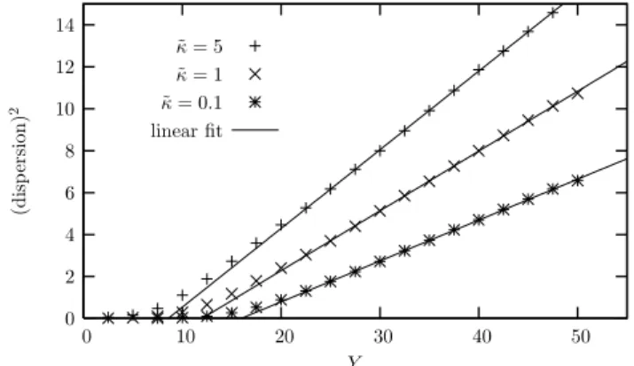
FIG. 10: Dispersion (squared) of the position of the events as a func-tion of rapidity. As expected, it dispersion increases like√Y but few dispersion is obtained in early stages of the evolution.
BK ˜
κ= 1 ˜
κ= 0.1
k
T
1025
1020
1015
1010
105
1 10
1
0.1
0.01
0.001
10−4
10−5
FIG. 11: Evolution of the averaged amplitude for different values of the noise strength, compared with the mean field result (dot-ted curve). The curves correspond, from left to right, to Y = 0,10,20,30,40 and 50.
physical units) fluctuates. At a give rapidity, one can compute the dispersion of those events. This diffusion process being very similar to a random walk, one expects that the dispersion of the events behaves like√Y:
X2Y− XY2Y→≈∞DdiffY.
The parametric dependence of the diffusion coefficient Ddiff has been computed numerically [20] and behaves9 like
|log−3(κα2
s)|.
Concerning the numerical simulations, the dispersion of the wavefront between different events and its increase with ra-pidity are manifest on figure 9. One can then extract the dis-persion as a function of rapidity. The resulting curve, shown on figure 10 for different values of the noise strength, calls for two remarks. First, the expected asymptotic behaviour (dispersion ∝√Y) is observed and the diffusion coefficient
9Recently, this coefficient has been computed analytically [22].
increases with rapidity. However, for small values of the ra-pidity, we do not observe a significant dispersion.
This dispersion of the events has an important physical consequences: although each single event displays geometric scaling, once we compute the average amplitude, dispersion induces geometric scaling violations10. This effect is best seen on figure 11 where we have compared the evolution with fluc-tuations to the BK results. While in the BK equation, a fixed travelling-wave pattern is formed, once fluctuations are take into account, we see a broadening of the average amplitude as rapidity increases.
V. DISCUSSION AND PERSPECTIVES
Let us now summarise the main points raised in these pro-ceedings. As this document is in itself some kind of a sum-mary, I shall only pick up the main points and refer to various references for detailed approaches.
First, we have shown that it is possible to describe the evo-lution to high energy in pQCD by a hierarchy of equations (see (8)). This gives the evolution of the Tmatrix (aver-aged over the target wave-function) and its higher-order corre-lationsTk. In this hierarchy, the evolution ofTkcontains three types of contribution:
1. the linear BFKL growth, proportional to ¯α
Tk. This is the usual high-energy contribution computed thirty years ago and corresponding to the exchange ofkpQCD pomerons. It leads to a fast (exponential) increase of the scattering amplitude.
2. the saturation corrections, proportional to ¯α
Tk+1
. This negative term becomes important when the ampli-tude reaches unitarity and it allows for the constraint T(r,b)≤1 to be satisfied.
3. the fluctuations term, proportional to ¯αα2
s
Tk−1. These fluctuations correspond to gluon-number fluctu-ations in the target. They play an important role when the amplitude is of orderα2
s or, equivalently, when the
dipole density is of order one,i.e. in the dilute regime where one indeed expects fluctuation effects to appear. If one neglects the fluctuation contributions, we recover the Balitsky hierarchy (in its large-Nc formulation) and, in the
mean field approximation, the BK equation is obtained. This last equation, much simpler than the infinite hierarchy cap-tures many important points concerning the physics of satura-tion. We also have to point out that, as long as we do not take into account fluctuations, the evolution at all orders in 1/Nc
exists under the form of the Balitsky/JIMWLK equation. We have only given a short introduction to the Colour Glass Con-densate (in which the JIMWLK equation is derived). Further
information concerning the Balitsky (resp. CGC) approach can be found if reference [24] (resp. [25]).
Many additional things can be said concerning those dif-ferent contributions,e.g.concerning the equivalence between descriptions from the target and projectile point of view (see e.g.[26]), or the attempts to describe the evolution beyond its large−Nclimit [27]. Again, the interested reader is forwarded
to the corresponding references (and the references therein) for further information.
In the second part of this overview, we have concentrated ourselves on the physical consequences arising from satura-tion and fluctuasatura-tion effects. We have searched how those con-tributions manifest themselves on the scattering amplitude and change the exponential behaviour obtained from the BFKL evolution. Again, the most important points can be sum-marised in two major steps with their respective physical con-sequences:
1. Considering BFKL with saturation effects (mean-field picture), one can show that the BK equation lies in the same universality class as the FKPP equation. This im-plies that travelling waves are formed during the evolu-tion towards high energy. From the BFKL kernel one obtains the critical parameters which are the anomalous dimension observed in the large-Q2tail and the speed of the wave, equivalent to the exponent of the saturation scale. In physical terms, these travelling waves corre-sponds to geometric scaling. The experimental obser-vation at HERA can thus be seen as a consequence of saturation. It is extremely important to realise that geo-metric scaling is a prediction from saturation physics which extends to large values ofQ2, far beyond the sat-uration scale itself11. This geometric scaling has also been predicted at nonzero momentum transfer, a result which may be applied for example toρ-meson produc-tion or DVCS.
2. If one includes the effects of fluctuations, the evolution becomes a Langevin equation12 equivalent to the sto-chastic FKPP equation, including a noise term. For each realisation of this noise, we observe geometric scaling with a decrease of the speed w.r.t. the mean-field case. If we consider a bunch of events, we observe that, although they all have the same shape, their po-sition is diffused with diffusion going like √Y. This dispersion of the saturation scale for a set of events
im-plies that geometric scaling is violated for the averaged amplitude. Numerical studies indicate that geometric scaling is still valid at small rapidities. At higher ener-gies, a new (diffusive) scaling is predicted [23] in which the amplitude scales like log(k2/Q2s(Y))/√Y.
These two pictures, although they endow most of the phys-ical effects, are far from being totally understood. Among the improvements, one can quote phenomenological applications like geometric ad diffusive scaling predictions for vector-meson productions, for diffraction [23] and for LHC physics. On more theoretical grounds most of the work needed to be done concerns the effects of fluctuations. Most of the results known so far are derived within the local approximation for the noise term and neglecting the impact parameter depen-dence. In addition, apart from numerical studies, analytical results can only be applied to irrealistically small values of
αsand a better understanding for more physical values is still
lacking. Although the existing picture is expected to contain the qualitative effects, a more precise treatment is certainly an interesting problem to address.
Within the framework presented here, the link between the QCD evolution equations and equations from statistical physics has led to a large number of interesting ideas and results. Even in statistical physics, many questions are yet opened, hence, extending the QCD picture including more so-phisticated treatments of the BFKL kernel and more precise forms of the noise term is certainly not a straightforward task. The questions of making clear predictions for phenomenol-ogy, of understanding the effects of fluctuations beyond the local-noise approximation and of including impact-parameter dependence are hence expected to give interesting work in the near future. Among particle physics, high-energy QCD is thus one of the most active fields. Because of those open questions and because of the requirement for an excellent knowledge of QCD at the LHC, we expect that high-energy QCD is still going to be active in the near future.
Acknowledgments
I would like to thank warmly the members of the Brazilian Particle Physics Society, and especially Beatriz Gay Ducati and Magno Machado, for the invitation to give a talk in this meeting. G.S. is funded by the National Funds for Scientific Research (FNRS), Belgium.
11The geometric scaling window grows, in logarithmic units, like√Ybeyond
the saturation scale.
12If one consider the complete evolution equation with full phase-space
de-pendence, one can also rewrite the hierarchy under the form of a Langevin
equation. It is also possible [28] to view the evolution s a reaction-diffusion process.
[1] V.N. Gribov and L.N. Lipatov, Sov. J. Nucl. Phys. 15, 438 (1972); G. Altarelli and G. Parisi, Nucl. Phys. B126, 298 (1977); Yu.L. Dokshitzer, Sov. Phys. JETP46, 641 (1977). [2] L. N. Lipatov, Sov. J. Nucl. Phys.23, 338 (1976); E. A. Kuraev,
L. N. Lipatov, and V. S. Fadin, Sov. Phys. JETP45, 199 (1977); I. I. Balitsky and L. N. Lipatov, Sov. J. Nucl. Phys. 28, 822
(1978).
[3] L. V. Gribov, E. M. Levin, and M. G. Ryskin, Phys. Rep.100, 1 (1983).
[4] I. I. Balitsky, Nucl. Phys. B463, 99 (1996) [arXiv:hep-ph/9509348];
Nucl. Phys. B 504, 415 (1997) [arXiv:hep-ph/9701284]; E. Iancu, A. Leonidov and L. D. McLerran, Nucl. Phys. A692, 583 (2001) [arXiv:hep-ph/0011241]; H. Weigert, Nucl. Phys. A 703, 823 (2002) [arXiv:hep-ph/0004044].
[6] Y. V. Kovchegov, Phys. Rev. D60, 034008 (1999) [arXiv:hep-ph/9901281]; Y. V. Kovchegov, Phys. Rev. D61, 074018 (2000), [arXiv:hep-ph/9905214].
[7] S. Munier and R. Peschanski, Phys. Rev. Lett. 91, 232001 (2003) [arXiv:hep-ph/0309177]; Phys. Rev. D69, 034008 (2004) [arXiv:hep-ph/0310357]; Phys. Rev. D70, 077503 (2004) [arXiv:hep-ph/0310357].
[8] R. A. Fisher, Ann. Eugenics7, 355 (1937); A. Kolmogorov, I. Petrovsky, and N. Piscounov, Moscou Univ. Bull. Math. A1, 1 (1937).
[9] A. M. Sta´sto, K. Golec-Biernat, and J. Kwiecinski, Phys. Rev. Lett.86, 596 (2001) [arXiv:hep-ph/0007192].
[10] A. H. Mueller and A. I. Shoshi, Nucl. Phys. B692, 175 (2004) [arXiv:hep-ph/0402193];
[11] E. Iancu, A. H. Mueller, and S. Munier, Phys. Lett. B606, 342 (2005) [arXiv:hep-ph/0410018].
[12] E. Iancu and D. N. Triantafyllopoulos, Nucl. Phys. A756, 419 (2005) [arXiv:hep-ph/0411405]. Phys. Lett. B610, 253 (2005) [arXiv:hep-ph/0501193].
[13] A. H. Mueller, A. I. Shoshi, and S. M. H. Wong, Nucl. Phys. B 715, 440 (2005) [arXiv:hep-ph/0501088].
[14] A. H. Mueller, Nucl. Phys. B415, 373 (1994); A. H. Mueller and B. Patel, Nucl. Phys. B425, 471 (1994); A. H. Mueller, Nucl. Phys. B437, 107 (1995).
[15] C. Marquet and G. Soyez, Nucl. Phys. A 760, 208 (2005) [arXiv:hep-ph/0504080].
[16] L. N. Lipatov, Sov. Phys. JETP63, 904 (1986) [Zh. Eksp. Teor. Fiz.90, 1536 (1986)]; H. Navelet and R. Peschanski, Nucl.
Phys. B507, 353 (1997) [arXiv:hep-ph/9703238].
[17] C. Marquet, R. Peschanski, and G. Soyez, Nucl. Phys. A756, 399 (2005) [arXiv:hep-ph/0502020].
[18] G. Soyez, Phys. Rev. D 72, 016007 (2005) [arXiv:hep-ph/0504129].
[19] R. Enberg, K. Golec-Biernat and S. Munier, Phys. Rev. D72, 074021 (2005) [arXiv:hep-ph/0505101].
[20] E. Brunet and B. Derrida, Phys. Rev. E57, 2597 (1997) [arXiv:cond-mat/0005362]; Comp. Phys. Comm. 121 376 (1999) [arXix:cond-mat/0005364]
[21] C. Marquet, R. Peschanski, and G. Soyez, arXiv:hep-ph/0512186.
[22] E. Brunet, B. Derrida, A. H. Mueller, and S. Munier, arXiv:cond-mat/0512021.
[23] Y. Hatta, E. Iancu, C. Marquet, G. Soyez, and D. N. Triantafyl-lopoulos, arXiv:hep-ph/0601150.
[24] I. Balitsky, arXiv:hep-ph/0101042.
[25] E. Iancu, A. Leonidov, and L. D. McLerran, Nucl. Phys. A 692, 583 (2001) [arXiv:hep-ph/0011241]; E. Ferreiro, E. Iancu, A. Leonidov, and L. McLerran, Nucl. Phys. A703, 489 (2002) [arXiv:hep-ph/0109115].
[26] A. Kovner and M. Lublinsky, Phys. Rev. D72, 074023 (2005) [arXiv:hep-ph/0503155].
[27] A. Kovner and M. Lublinsky, Phys. Rev. D71, 085004 (2005) [arXiv:hep-ph/0501198], Phys. Rev. Lett. 94, 181603 (2005) [arXiv:hep-ph/0502119]; Y. Hatta, E. Iancu, L. McLerran, and A. Stasto, Nucl. Phys. A 762, 272 (2005) [arXiv:hep-ph/0505235]; Y. Hatta, E. Iancu, L. McLerran, A. Stasto, and D. N. Triantafyllopoulos, Nucl. Phys. A764, 423 (2006) [arXiv:hep-ph/0504182].
![FIG. 4: One step of JIMWLK evolution: the emitted soft gluon prop- prop-agating in the string target field is used to redefine the probability W [ρ] at rapidity Y + δY](https://thumb-eu.123doks.com/thumbv2/123dok_br/18981805.457302/3.892.480.825.80.192/jimwlk-evolution-emitted-agating-string-redefine-probability-rapidity.webp)