Submitted10 October 2016 Accepted 1 December 2016 Published12 January 2017
Corresponding author
Yumin Guo, [email protected]
Academic editor Stuart Pimm
Additional Information and Declarations can be found on page 17
DOI10.7717/peerj.2849
Copyright 2017 Mi et al.
Distributed under
Creative Commons CC-BY 4.0
OPEN ACCESS
Why choose Random Forest to predict
rare species distribution with few samples
in large undersampled areas? Three Asian
crane species models provide supporting
evidence
Chunrong Mi1, Falk Huettmann2, Yumin Guo1, Xuesong Han1and Lijia Wen1 1College of Nature Conservation, Beijing Forestry University, Beijing, China
2EWHALE Lab, Department of Biology and Wildlife, Institute of Arctic Biology, University of Alaska Fairbanks (UAF), Fairbanks, AK, United States
ABSTRACT
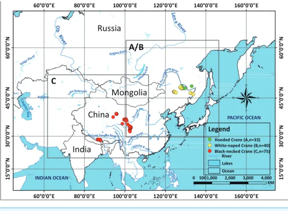
Species distribution models (SDMs) have become an essential tool in ecology, bio-geography, evolution and, more recently, in conservation biology. How to generalize species distributions in large undersampled areas, especially with few samples, is a fundamental issue of SDMs. In order to explore this issue, we used the best available presence records for the Hooded Crane (Grus monacha,n=33), White-naped Crane (Grus vipio,n=40), and Black-necked Crane (Grus nigricollis,n=75) in China as three case studies, employing four powerful and commonly used machine learning algorithms to map the breeding distributions of the three species: TreeNet (Stochastic Gradient Boosting, Boosted Regression Tree Model), Random Forest, CART (Classification and Regression Tree) and Maxent (Maximum Entropy Models). In addition, we developed an ensemble forecast by averaging predicted probability of the above four models results. Commonly used model performance metrics (Area under ROC (AUC) and true skill statistic (TSS)) were employed to evaluate model accuracy. The latest satellite tracking data and compiled literature data were used as two independent testing datasets to confront model predictions. We found Random Forest demonstrated the best performance for the most assessment method, provided a better model fit to the testing data, and achieved better species range maps for each crane species in undersampled areas. Random Forest has been generally available for more than 20 years and has been known to perform extremely well in ecological predictions. However, while increasingly on the rise, its potential is still widely underused in conservation, (spatial) ecological applications and for inference. Our results show that it informs ecological and biogeographical theories as well as being suitable for conservation applications, specifically when the study area is undersampled. This method helps to save model-selection time and effort, and allows robust and rapid assessments and decisions for efficient conservation.
SubjectsBiodiversity, Biogeography, Conservation Biology, Ecology, Zoology
Keywords Species distribution models (SDMs), Random Forest, Generality (transferability),
Rare species, Undersampled areas, White-naped crane (Grus vipio), Black-necked crane (Grus
INTRODUCTION
Species distribution models (SDMs) are empirical ecological models that relate species observations to environmental predictors (Guisan & Zimmermann, 2000;Drew, Wiersma & Huettmann, 2011). SDMs have become an increasingly important and now essential tool in ecology, biogeography, evolution and, more recently, in conservation biology (Guisan et al., 2013), management (Cushman & Huettmann, 2010), impact assessments (Humphries & Huettmann, 2014) and climate change research (Lei et al., 2011;Mi, Huettmann & Guo, 2016). To generalize and infer from a model, or model transferability is defined as geograph-ical or temporal cross-applicability of models (Thomas & Bovee, 1993;Kleyer, 2002;Randin et al., 2006). It is one important feature in SDMs, a base-requirement in several ecological and conservation biological applications (Heikkinen, Marmion & Luoto, 2012). In this study, we used generality (transferability) as the concept of generalizing distribution from sampled areas to unsampled areas (extrapolation beyond the data) in one study area.
Detailed distribution data for rare species in large areas are rarely available in SDMs ( Pear-son et al., 2007;Booms, Huettmann & Schempf, 2010). However, they are among the most needed for their conservation to be effective. Collecting and assembling distribution data for species, especially for rare or endangered species in remote wilderness areas is often a very difficult task, requiring a large amount of human, time and funding sources (Gwena et al., 2010;Ohse et al., 2009).
Model generality (transferability) testing could offer particularly powerful for model evaluation (Randin et al., 2006). Independent observations from a training data set has been recommended as a more proper evaluations of models (Fielding & Bell, 1997;Guisan & Zimmermann, 2000). Therefore, the use of an independent geographically (Fielding & Haworth, 1995) or temporally (Boyce et al., 2002; Araújo et al., 2005) testing data set is encouraged to assess the generality of different SDMs techniques. Data from museum specimen, published literature (Graham et al., 2004) as well as tracking are good source to assess model generality (transferability) performance. In addition, how the distribution map links with reality data, especially in undersampled areas where modelers want to make predictions should definitely be employed as a metric to assess model performance and generalization. Arguably, if model predictions perform very well there, great progress is provided and usually done cost-effective too. However, predictions on existing knowledge and data offer less progress. The model prediction and conservation frontier obviously sits in the unknown and to provide progress there (Breiman, 2001;Drew, Wiersma & Huettmann, 2011).
In this study, we investigated models for the best-available data for three species in East Asia as test cases: Hooded Cranes (Grus monacha,n=33), White-naped Cranes (Grus vipio,
n=40) and Black-necked Cranes (Grus nigricollis,n=75). Four machine-learning model algorithms (TreeNet, Random Forest, CART and Maxent) were applied to map breeding distributions for these three crane species which otherwise lack empirically derived distribution information. In addition, two kinds of independent testing data sets (latest satellite tracking data, and compiled literature data (Threatened Birds of Asia:Collar, Crosby & Crosby, 2001) were obtained to test the transferability of the four model algorithms. The purpose of this investigation is to explore whether there is a SDM technique among the four algorithms that could generate reliable and accurate distributions with high generality for rare species using few samples but in large undersampled areas. Results from this research could be useful for the detection of rare species and enhance fieldwork sampling in large undersampled areas which would save money and effort, as well as advance the conservation management of those species.
MATERIALS AND METHODS
Species data
In our 13 combined years of field work, we have collected 33 Hooded Crane nests (2002– 2014), 40 White-naped Crane nests (2009–2014) (Supplemental Information 2), and 75 Black-necked Crane nests (2014) (seeFig. 1), during breeding seasons. We used these field samples (nests) to represent species presence points referenced in time and space.
Environmental variables
! ( ! (!( ! (!( ! (!(!(!(!(!( ! (!(!(!( ! (((!!!(!!((!((!(!!((!(!(!(! ! (!(!( !( ! ( ! ( ! ( ! ( ! ( ! ( ! ( !(!(!(!(!( ! ( ! ( ! ( ! ( ! ( ! ((!(!(!(!!(!(!(!((! ! ( ! (!(!(!((!(!!(!(!( !( ! ( ! ( ! ( ! ((!(!(!(!(!!!(((!!(!(!(!( ! ( ! ( ! ( ! ( ! ( ! ( ! ( ! ( ! ( ! ( ! ((!(!(!(!!!(!!(((!(!(!(!(!(!( ! ( ! ( ! ( ! ( ! ( ! ( ! ( ! ( ! ( ! ( ! ( ! ( ! ( ! ( ! (!( ! ( ! ( ! ( ! (!(!(!(!( ! (!( ! ( ! ( ! ( ! ( ! ( ! ( ! ( ! (!(!( 160°0'0"E 160°0'0"E 140°0'0"E 140°0'0"E 120°0'0"E 120°0'0"E 100°0'0"E 100°0'0"E 80°0'0"E 80°0'0"E 60°0'0"E 60°0'0"E 60°0'0"N 60°0'0"N 45°0'0"N 45°0'0"N 30°0'0"N 30°0'0"N 15°0'0"N 15°0'0"N
C
A/B
0 5001,000 2,000 3,000 4,000 KM
®
China
Russia
Mongolia
India
Le n a Riv er O b Riv er AngaraRiver He ilo ngjiang River
Yel l
ow R
iv
e
r
Yang
tzeR iv
er
Xijiang River
Yar lung Zangbo RiverLancan
g R ive r Volga River C asp ian Se a
Aral Sea La
ke Balk hash
Lake Ba ika l Text INDIAN OCEAN PACIFIC OCEAN Legend ! ( ! ( ! ( River Lakes Ocean
White-naped Crane (B,n=40) Hooded Crane (A,n=33)
Black-necked Crane (C,n=75)
Figure 1 Study areas for three species cranes.
land cover factors (for detailed information, seeTable 1). Most of these predictors were obtained from open access sources. Bio-climate factors were obtained from the WorldClim database (http://www.worldclim.org), while aspect and slope layer were derived from the altitude layer in ArcGIS, which was also initially obtained from the WorldClim database. Road, railroad, river, lake and coastline and settlement maps were obtained from the Natural Earth database (http://www.naturalearthdata.com). The land cover map was obtained from the ESA database (http://www.esa-landcover-cci.org). We also made models with all 19 bio-climate variables and 10 other environmental variables, and then reduced predictors by AIC, BIC, varclust, PCA and FA analysis. When we compared the distribution maps overlaying with independent data set generated by Random Forest model, we found the model based on 21 predictors have the best performance for Hooded Cranes, and the best level for White-naped Crane and Black-necked Cranes (seeTable S1). Therefore, we decided to constructed models with 21 predictors for the all three cranes and four machine-learning techniques. All spatial layers of these environmental variables were resampled in ArcGIS to a resolution of 30-s to correspond to that of the bioclimatic variables and for a meaningful high-resolution management scale.
Model development
Table 1 Environmental GIS layers used to predict breeding distributions of three cranes.
Environmental layers
Description Source Website
Bio_1 Annual mean temperature (◦C) WorldClim http://www.worldclim.org/
Bio_2 Monthly mean (max temp–min temp) (◦
C) WorldClim http://www.worldclim.org/
Bio_3 Isothermality (BIO2/BIO7) (*100◦C) WorldClim http://www.worldclim.org/
Bio_4 Temperature seasonality (standard deviation *100◦
C)
WorldClim http://www.worldclim.org/
Bio_5 Max temperature of warmest month (◦C) WorldClim http://www.worldclim.org/
Bio_6 Min temperature of coldest month (◦C) WorldClim http://www.worldclim.org/
Bio_7 Annual temperature range (BIO5-BIO6) (◦
C) WorldClim http://www.worldclim.org/
Bio_12 Annual precipitation (mm) WorldClim http://www.worldclim.org/
Bio_13 Precipitation of wettest month (mm) WorldClim http://www.worldclim.org/
Bio_14 Precipitation of driest month (mm) WorldClim http://www.worldclim.org/
Bio_15 Precipitation seasonality (mm) WorldClim http://www.worldclim.org/
Altitude Altitude (m) WorldClim http://www.worldclim.org/
Aspect Aspect (◦
) Derived from Altitude http://www.worldclim.org/
Slope Slope Derived from Altitude http://www.worldclim.org/
Landcover Land cover ESA http://www.esa-landcover-cci.org/
Disroad Distance to roads (m) Road layer from Natural Earth http://www.naturalearthdata.com/
Disrard Distance to railways (m) Railroad layer from Natural Earth http://www.naturalearthdata.com/
Disriver Distance to rivers (m) River layer from Natural Earth http://www.naturalearthdata.com/
Dislake Distance to lakes (m) Lake layer from Natural Earth http://www.naturalearthdata.com/
Discoastline Distance to coastline (m) Coastline layer from Natural Earth http://www.naturalearthdata.com/
Dissettle Distance to settlements (m) Settle layer from Natural Earth http://www.naturalearthdata.com/
performing machine learning methods (more information about these four models can be seen in the references byBreiman et al., 1984;Breiman, 2001;Friedman, 2002;Phillips, Dudík & Schapire, 2004;Hegel et al., 2010). The first three machine learning models are binary (presence-pseudo absence) models and were handled in Salford Predictive Modeler 7.0 (SPM). For more details on TreeNet, Random Forest and CART in SPM and their performances, we refer readers to the user guide document online (
https://www.salford-systems.com/products/spm/userguide). Several implementations of these algorithms exist.
visualization, we imported the dataset of spatially referenced predictions (‘score file’) into GIS as a raster file and interpolated for visual purposes between the regular points using inverse distance weighting (IDW) to obtain a smoothed predictive map of all pixels for the breeding distributions of the three cranes (as performed inOhse et al., 2009;Booms, Huettmann & Schempf, 2010). The fourth algorithm we employed, Maxent, is commonly referred to as a presence-only model; we used Maxent 3.3.3 k (it can be downloaded for free fromhttp://www.cs.princeton.edu/~schapire/maxent/) to construct our models. To run Maxent, we followed the 3.3.3e tutorial for ArcGIS 10 (Young, Carter & Evangelista, 2011) and used default settings.
Testing data and model assessment
We applied two types of testing data in this study: one consisted of satellite tracking data, and the other was represented by data from the literature. Satellite tracking data were obtained from four individual Hooded Cranes and eight White-naped Cranes that were tracked at stopover sites (for more details regarding the information for tracked cranes, please see
Fig. S1). The satellite tracking devices could provide 24 data points per day (Supplemental
Information 4). Here, we chose points that had a speed of less than 5 km/h during the period
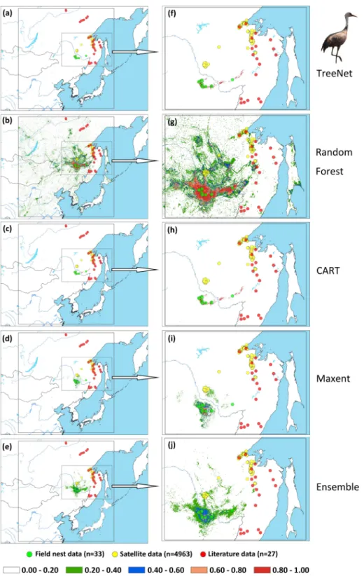
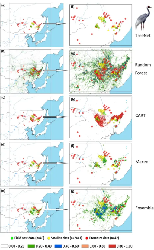
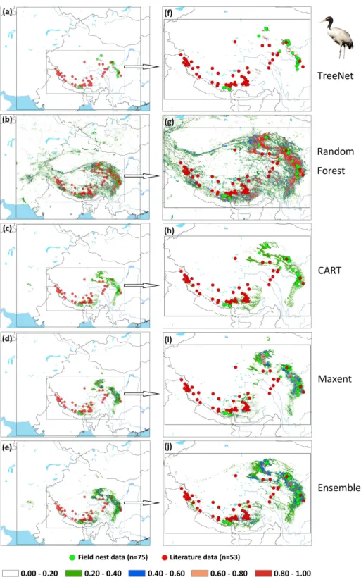
from 1st May to 31th June for Hooded Cranes and 15th April to 15th June for White-naped Cranes as the locations of the breeding grounds for these two cranes. The total numbers of tracking data points were 4,963 and 7,712 (Hooded Cranes and White-naped Crane, respectively. We didn’t track Black-necked Cranes, so there was no tracking testing data for this species.). The literature data for this study were obtained by geo-referencing the location points of detections from 1980–2000 (ArcGIS 10.1) from Threatened Birds of Asia: the BirdLife International Red Data Book (Collar, Crosby & Crosby, 2001). From this hardcopy data source, we were able to obtain and digitize 27 breeding records for Hooded Cranes, 43 breeding records for White-naped Cranes, and 53 breeding records for Black-necked Cranes (see Figs. 2A–2CandSupplemental Information 3). Here we digitized the only available crane data for these three species in East-Asia into a database.
In addition, we generated 3,000 random points for Hooded Cranes and White-naped Cranes, and 5,000 random points for Black-necked Cranes as testing pseudo-absence points in their respective study areas; then, the literature locations (additional presence points for testing) and random points locations (testing absence points) that contrasted with the associated predictive value of RIO extracted from the relative prediction map, which were used to calculate receiver operating characteristic (ROC) curves and the true skill statistic (TSS) (Hijmans & Graham, 2006). The area under the ROC curve (AUC) is commonly used to evaluate models in species distributional modeling (Manel, Williams & Ormerod, 2001; McPherson, Jetz & Rogers, 2004). TSS was also used to evaluate model performance; we used TSS because it has been increasingly applied as a simple but robust and intuitive measure of the performance of species distribution models (Allouche, Tsoar & Kadmon, 2006).
Hooded Crane
White-naped Crane
Black-necked Crane
Figure 2 Detailed study areas showing the presence of and testing data used for the three cranes.(A)
Table 2 AUC and TSS values for four machine learning models and their Ensemble model with three crane species based on literature testing data.
Accuracy metric (samples) Species distribution model
TreeNet Random Forest CART Maxent Ensemble
Hooded Crane (Grus monacha, n=33 sites)
AUC 0.504 0.625 0.500 0.558 0.558
TSS 0.000 0.250 0.000 0.137 0.117
White-naped Crane (Grus vipio,n=40 sites)
AUC 0.605 0.754 0.564 0.712 0.754
TSS 0.210 0.509 0.128 0.424 0.508
Black-necked Crane (Grus nigricollis,n=75 sites)
AUC 0.528 0.830 0.672 0.805 0.843
TSS 0.055 0.660 0.345 0.611 0.686
based on the local area with samples to predict into undersampled areas that are otherwise unsampled in the model development (=areas without training data). In addition, AUC is also commonly used to assess model transferability in our study referringRandin et al. (2006).
RESULTS
Model performance
The results for AUC and TSS, two metrics commonly used to evaluate model accuracy, are listed inTable 2. For the four SDMs technique, our results showed that the AUC values for Random Forest were always highest (>0.625), ranking this model in first place, followed by Maxent (>0.558), and then either CART or TreeNet (≥0.500). TSS showed us consistent
results, as was the case for AUC, and Random Forest performed the best (>0.250) followed by Maxent (>0.137) for all three crane species, CART took the third place for Black-necked Cranes, and TreeNet performed better than CART for White-naped Cranes. And the results showed there was a trend that the value of these three metrics increased with an increase of nest site samples (33–75, Hooded Crane to Black-necked Crane, seeTable 2). Comparing the results of Random Forest with Ensemble models, we found their performance were close. Random Forest obtained better models for Hooded Cranes and White-naped Cranes cases, the Ensemble model performed better for Black-necked Cranes.
Model generalization
Relatieve
Index
of
Occurrence
0.
0
0.
2
0.
4
0.
6
0.
8
1.
0
0.
0
0.
2
0.
4
0.
6
0.
8
1.
0
TreeNet Random Forest CART Maxent Ensemble
White-naped Crane Hooded Crane
Model
(a)
(b)
Figure 3 Violin plots of the Relative Index of Occurrence (RIO) for four SDMs and Ensemble model
for Hooded Cranes and White-naped Cranes based on satellite tracking data.(A) Violin plots of
Hooded Cranes, (B) violin plots of White-naped Cranes.
Maxent (median was 0.37) and then Ensemble and CART. While some tracking points had a low RIO value in TreeNet, the majority of RIO values for CART remained in the 0.20 range.
Violin plots of the RIOs values for the three cranes extracted for the literature data from the prediction maps (Fig. 4) demonstrated consistent trends (Fig. 3), indicating that Random Forest performed best across all models of the three species. InFig. 4A, the RIO values for Random Forest ranged from 0 to 0.48, and most RIO values were below 0.1; the RIO values for the other three SDMs method were 0, the Ensemble model performed a little bit better. As showed inFig. 4B, most RIO values for Random Forest were below 0.7, and the median value was approximately 0.20, followed by Maxent and then CART. The violin plots for Black-necked Cranes (Fig. 4C) indicated that TreeNet performed the worst, although there were some pixels that had high RIO values, followed by the Ensemble model and then Maxent. The best performer was still Random Forest, and its RIOs were distributed evenly to a certain extent with a median value of 0.44. The results of AUC, as mentioned in the ‘‘Model performance’’ section (Table 2), showed consistent results with violin plots, and Random Forest always achieved the highest value and had the best generalization.
Spatial assessment using a testing data overlay prediction map
Model
0.
0
0.
2
0.
4
0.
6
0.
8
1.
0
0.
0
0.
2
0.
4
0.
6
0.
8
1.
0
0.
0
0.
2
0.
4
0.
6
0.
8
1.
0
TreeNet Random Forest CART Maxent Ensemble
Relative Index of Occurrence
Hooded Crane (a)
White-naped Crane
Black-necked Crane (b)
(c)
Figure 4 Violin plots of Relative Index of Occurrence (RIO) values for four SDMs and Ensemble
model for three cranes based on calibration data from Threatened Birds of Asia.(A) Violin plots for
Hooded Cranes, (B) violin plots for White-naped Cranes, (C) violin plots for Black-necked Cranes.
of model performance. It is a spatial and visual method to show the transferability of SDMs from sampled to unsampled areas. From the results (Figs. 5,6, 7andSupplemental
Information 1), we found that Random Forest demonstrated the strongest performance
Figure 5 Prediction maps for Hooded Cranes and zoomed-in maps showing the four models (TreeNet,
Random Forest, CART and Maxent) and Ensemble model in detail.(A–E) Prediction map for Hooded
Figure 6 Prediction maps for White-naped Cranes and zoomed-in maps showing the four models
(TreeNet, Random Forest, CART and Maxent) and Ensemble model in detail.(A–E) Prediction map for
Figure 7 Prediction maps for Black-necked Cranes and zoomed-in maps showing the four models
(TreeNet, Random Forest, CART and Maxent) and Ensemble model in detail.(A–E) Prediction map for
DISCUSSION
Model generality (transferability)
Estimating species distributions in undersampled areas is a fundamental problem in ecology, biogeography, biodiversity conservation and natural resource management (Drew, Wiersma & Huettmann, 2011). That is specifically true for rare and difficult to be detected species and which are usually high on the conservation priority. The use of SDMs and with machine learning has become the method for deriving such estimates (Guisan & Thuiller, 2005;Drew, Wiersma & Huettmann, 2011;Guisan et al., 2013) and could contribute to detect new and to confirm populations of rare species. However, the application of a few samples to project a distribution area widely beyond the sample range is a greater challenge and has rarely been attempted in the literature until recently. Only now have
conservationists realized its substantial value for pro-active decision making in conservation management (see work byOhse et al., 2009;Drew, Wiersma & Huettmann, 2011;Kandel et al., 2015etc.). Our results based on AUC, violin plots for RIOs and spatial assessment of testing data (satellite tracking data and literature data) all suggest there are difference in the generalization performance of different modeling techniques (TreeNet, Random Forest, CART and Maxent).
Moreover, among the acknowledged four rather powerful and commonly used machne-learning techniques, Random Forest (bagging) in SPM usually had the best performance in each case. Our results are in agreement with those ofPrasad, Iverson & Liaw (2006),Cutler et al. (2007) andSyphard & Franklin (2009)indicating a superiority of Random Forest in such applications. However, initially it appears to run counter to the conclusions off recent paper (Heikkinen, Marmion & Luoto, 2012) with the poor transferability of Random Forest. But we propose this is due to the fact that many Random Forest implementations exist (see the 100 classifier paperFernández-Delgado et al., 2014).
Here we applied Random Forest in SPM which has been optimized under one of the algo-rithm’s original co-authors, whileHeikkinen, Marmion & Luoto (2012)run a basic Random Forest with BIOMOD framework in the R sofeware and which remains widely un-tuned and largely behind the potential. The differences are known to be rather big (seeHerrick, 2013for a comparison).
Furthermore, Maxent, a widely used SDM-method consequently greatly enjoyed by many modelers (Phillips, Anderson & Schapire, 2006;Peterson, Monica & Muir, 2007; Phillips & Dudík, 2008;Li et al., 2015, and so on), didn’t perform so good in regards to transferability in this study. This contrasts to those ofElith et al. (2006)andHeikkinen, Marmion & Luoto (2012), where Maxent and GBM (generalized boosting methods) perform well. We infer this may be caused by sample size used as training data and due to the actual algorithms used. When the sample size increased (33–75), the AUC and TSS value of all models rose (Table 2). This indicates that higher sample sizes make models more robust and performing better. Sample sizes of 33 presence points still favor by Random Forest.
the best predictor from a very small, randomly chosen subset of the predictor variable pool (Herrick, 2013). These trees comprising the forest are each grown to maximal depth, and predictions are made by averaged trees through ‘voting’ (Breiman, 2001). This algorithm avoids overfitting by controlling the number of predictors randomly used at each split, using means of out-of-bag (OOB) samples to calculate an unbiased error rate. And also, Random Forest in SPM utilizes additional specific fine-tuning for best performance.
RIOs of random points
In order to explore whether Random Forest created higher RIOs for prediction maps in each grid, which would result into higher RIOs of testing data, we generated 3,000 random points for Hooded Cranes and White-naped Cranes, 5,000 random points for Black-necked Cranes in their related projected study areas. We made violin plots for RIOs of random points (Fig. 8), and we found that more RIO values of random points for Maxent, Random Forest and Ensemble models were close to the lower value, and then followed by TreeNet. The distribution shapes of Random Forest, Maxent and Ensemble model are more similar to the real distribution of species in the real world. The RIOs of White-naped Crane extracted from the CART model distributed in the range of the low value; this means there were no points located in the high RIO areas of cranes, which is unrealistic. Consequently, we argued that Random Forest did not create higher RIOs for prediction maps in each grid in our study.
Models with small sample sizes
Conservation biologists are often interested in rare species and seek to improve their conservation. These species typically have limited number of available occurrence records, which poses challenges for the creation of accurate species distribution models when compared with models developed with greater numbers of occurrences (Stockwell & Peterson, 2002;McPherson, Jetz & Rogers, 2004;Hernandez et al., 2006). In this study, we used three crane species as case studies, and their occurrence records (nests) totaled 33, 40, and 75, respectively (considering the small numbers of samples and given that a low fraction of the area was sampled in the large projected area). In our models, we found that model fit (AUC and TSS, seeTable 2) of Random Forest that had the highest index, while Maxent usually ranked second. In addition, we found that models with few presence samples can also generate accurate species predictive distributions (Figs. 3–7) with the Random Forest method. Of course, models constructed with few samples underlie the threat of being biased more because few samples usually had not enough information including all distribution gradients conditions of a species, especially for places far away from the location of training presence points. However, the potential distribution area predicted by SDMs could become the place where scholars could look for the birds (additional fieldwork sampling). Also, these places could be used as diffusion or reintroduction areas! It is valuable and new information either way.
Evaluation methods
In this study, we applied two widely-used assessment methods (AUC and TSS) in SDMs
(Table 2). For an evaluation of these three values we used the approach recommended by
Model
0.
0
0.
2
0.
4
0.
6
0.
8
1.
0
0.
0
0.
2
0.
4
0.
6
0.
8
1.
0
0.
0
0.
2
0.
4
0.
6
0.
8
1.
0
TreeNet Random Forest CART Maxent Ensemble
Rela!ve
Index
of
Occurrence
Hooded Crane (a)
White-naped Crane
Black-necked Crane (b)
(c)
Figure 8 Violin plots of Relative Index of Occurrence (RIO) values for four SDMs and Ensemble
model for three cranes based on calibration data from Threatened Birds of Asia.(A) Violin plots for
Hooded Cranes, (B) violin plots for White-naped Cranes, (C) violin plots for Black-necked Cranes.
effective (Drew & Perera, 2011), albeit nonstandard, evaluation methods (seeKandel et al., 2015for an example). Additionally, one alternative method for rapid assessment we find is to use a reliable SDM, and thus Random Forest would be a good choice in the future given our consistent results (Figs. 3–7) in this study, which involved three species, a vast landscape to conserve, and only limited data. Our work certainly helps to inform conservation decisions for cranes in Northeast Asia.
Limitations and future work
Our study is not without limitations: (1) so far, only three species of cranes are used as a test case in our study because nest data for rare species in remote areas are usually sparse, and; (2) all our species study areas are rather vast and confined to East-Asia. For future work, we would apply Random Forest in more species and in more geographical conditions with differently distributed features for a first rapid assessment and baseline to be mandatory for better conservation, e.g., by governments, IUCN and any impact and court decision. We would then apply our prediction results in specifically targeted fieldwork sampling campaigns and assess the model accuracy with field survey results (ground-truthing) and with new satellite tracking and drone data, for instance. This is to be fed directly into the conservation management process.
ACKNOWLEDGEMENTS
We thank Fengqin Yu, Yanchang Gu, Linxiang Hou, Jianguo Fu, Bin Wang, Jianzhi Li, Lama Tashi Sangpo, Baiyu Lamasery, and Nyainbo Yuze for their hard work in the field. Thanks to all data contributors to the book ‘Threatened Birds of Asia.’ Thanks to the support of State Forestry Administration and Whitley Fund for Nature (WFN). We also thank Salford Systems Ltd. (Dan Steinberg) for providing the free trial version of their data mining and machine learning software to the conservation research community. This is EWHALE lab publication #177.
ADDITIONAL INFORMATION AND DECLARATIONS
Funding
This Project is fund by the National Natural Science Foundation of China (No. 31570532). The funders had no role in study design, data collection and analysis, decision to publish, or preparation of the manuscript.
Grant Disclosures
The following grant information was disclosed by the authors: National Natural Science Foundation of China: No. 31570532.
Competing Interests
Author Contributions
• Chunrong Mi conceived and designed the experiments, performed the experiments, analyzed the data, contributed reagents/materials/analysis tools, wrote the paper, prepared figures and/or tables, reviewed drafts of the paper.
• Falk Huettmann conceived and designed the experiments, analyzed the data, wrote the paper, reviewed drafts of the paper.
• Yumin Guo, Xuesong Han and Lijia Wen contributed reagents/materials/analysis tools, reviewed drafts of the paper.
Data Availability
The following information was supplied regarding data availability: The raw data has been supplied asSupplementary File.
Supplemental Information
Supplemental information for this article can be found online athttp://dx.doi.org/10.7717/
peerj.2849#supplemental-information.
REFERENCES
Allouche OA, Tsoar, Kadmon R. 2006.Assessing the accuracy of species distribution models: prevalence, kappa and the true skill statistic (TSS).Journal of Applied Ecology
43(6):1223–1232DOI 10.1111/j.1365-2664.2006.01214.x.
Araújo MB, New M. 2007.Ensemble forecasting of species distributions.Trends in Ecology & Evolution22(1):42–47DOI 10.1016/j.tree.2006.09.010.
Araújo MB, Whittaker R, Ladle R, Erhard M. 2005.Reducing uncertainty in pro-jections of extinction risk from climate change.Global Ecology & Biogeography
14(6):529–538DOI 10.1111/j.1466-822X.2005.00182.x.
Beyer H. 2013.Hawth’s analysis tools for ArcGIS. Version 3.27.Available athttp:// www. spatialecology.com/ htools/ tooldesc.php.
Booms TL, Huettmann F, Schempf PF. 2010.Gyrfalcon nest distribution in Alaska based on a predictive GIS model.Polar Biology33(3):347–358
DOI 10.1007/s00300-009-0711-5.
Boyce MS, Vernier PR, Nielsen SE, Schmiegelow FK. 2002.Evaluating resource selection functions.Ecological Modelling 157(2–3):281–300
DOI 10.1016/S0304-3800(02)00200-4.
Breiman L. 2001.Random forests.Machine Learning 45(1):5–32
DOI 10.1023/A:1010933404324.
Breiman L, Friedman JH, Olshen RA, Stone CJ. 1984.Classification and regression trees. Boca Raton: CRC Press.
Collar NJ, Crosby R, Crosby M. 2001.Threatened birds of Asia: the BirdLife International
red data book. Volume 1. Cambridge: BirdLife International.
Cutler DR, Edwards Jr TC, Beard KH, Cutler A, Hess KT, Gibson J, Lawler JJ. 2007.
Random forests for classification in ecology.Ecology 88(11):2783–2792
DOI 10.1890/07-0539.1.
Drew CA, Perera AH. 2011. Expert knowledge as a basis for landscape ecological predictive models. In:Predictive species and habitat modeling in landscape ecology. New York: Springer, 229–248.
Drew CA, Wiersma Y, Huettmann F. 2011.Predictive species and habitat modeling in landscape ecology: concepts and applications. London: Springer.
Elith J, Graham CH, Anderson RP, Dudík M, Ferrier S, Guisan A, Hijmans RJ,
Huettmann F, Leathwick JR, Lehmann A, Li J, Lohmann LG, Loiselle BA, Manion G, Moritz C, Nakamura M, Nakazawa Y, Overton JMM, Peterson AT, Phillips SJ, Richardson K, Scachetti-Pereira R, Schapire RE, Soberón J, Williams S, Wisz MS, Zimmermann NE. 2006.Novel methods improve prediction of species’ distributions from occurrence data.Ecography29(2):129–151
DOI 10.1111/j.2006.0906-7590.04596.x.
Fernández-Delgado M, Cernadas E, Barro S, Amorim D. 2014.Do we need hundreds of classifiers to solve real world classification problems?The Journal of Machine
Learning Research15(1):3133–3181.
Fielding AH, Bell JF. 1997.A review of methods for the assessment of prediction errors in conservation presence/absence models.Environmental Conservation24(1):38–49
DOI 10.1017/S0376892997000088.
Fielding AH, Haworth PF. 1995.Testing the generality of bird-habitat models. Conserva-tion Biology9(6):1466–1481.
Friedman JH. 2002.Stochastic gradient boosting.Computational Statistics & Data
Analysis38(4):367–378DOI 10.1016/S0167-9473(01)00065-2.
Graham CH, Ferrier S, Huettman F, Moritz C, Peterson AT. 2004.New developments in museum-based informatics and applications in biodiversity analysis.Trends in Ecology & Evolution19(9):497–503DOI 10.1016/j.tree.2004.07.006.
Guisan A, Thuiller W. 2005.Predicting species distribution: offering more than simple habitat models.Ecology Letters8(9):993–1009
DOI 10.1111/j.1461-0248.2005.00792.x.
Guisan A, Tingley R, Baumgartner JB, Naujokaitis-Lewis I, Sutcliffe PR, Tulloch AIT, Regan TJ, Brotons L, Mcdonald-Madden E, Mantyka-Pringle C. 2013.Predicting species distributions for conservation decisions.Ecology Letters16(12):1424–1435
DOI 10.1111/ele.12189.
Guisan A, Zimmermann NE. 2000.Predictive habitat distribution models in ecology.
Ecological Modelling 135(2):147–186DOI 10.1016/S0304-3800(00)00354-9.
Gwena LL, Robin E, Erika F, Guisan A. 2010.Prospective sampling based on model ensembles improves the detection of rare species.Ecography33(6):1015–1027
DOI 10.1111/j.1600-0587.2010.06338.x.
in Alaskan waters: a first open-access ensemble model.Integrative and Comparative Biology51(4):608–622DOI 10.1093/icb/icr102.
Hegel TM, Cushman SA, Evans J, Huettmann F. 2010. Current state of the art for statistical modelling of species distributions. In:Spatial complexity, informatics, and wildlife conservation. Tokyo: Springer, 273–311.
Heikkinen RK, Marmion M, Luoto M. 2012.Does the interpolation accuracy of species distribution models come at the expense of transferability?Ecography35(3):276–288
DOI 10.1111/j.1600-0587.2011.06999.x.
Hernandez PA, Graham CH, Master LL, Albert DL. 2006.The effect of sample size and species characteristics on performance of different species distribution modeling methods.Ecography29(5):773–785DOI 10.1111/j.0906-7590.2006.04700.x.
Herrick K. 2013.Predictive modeling of Avian influenza in wild birds. PhD thesis, University of Alaska-Fairbanks (UAF).
Hijmans RJ, Graham CH. 2006.The ability of climate envelope models to predict the effect of climate change on species distributions.Global Change Biology
12(12):2272–2281DOI 10.1111/j.1365-2486.2006.01256.x.
Huettmann F, Gottschalk T. 2011. Simplicity, model fit, complexity and uncertainty in spatial prediction models applied over time: we are quite sure, aren’t we? In:
Predictive species and habitat modeling in landscape ecology. New York: Springer, 189–208.
Humphries GRW, Huettmann F. 2014.Putting models to a good use: a rapid assessment of Arctic seabird biodiversity indicates potential conflicts with shipping lanes and human activity.Diversity and Distributions20(4):478–490 DOI 10.1111/ddi.12177.
Kandel K, Huettmann F, Suwal MK, Regmi GR, Nijman V, Nekaris K, Lama ST, Thapa A, Sharma HP, Subedi TR. 2015.Rapid multi-nation distribution assessment of a charismatic conservation species using open access ensemble model GIS predictions: red panda (Ailurus fulgens) in the Hindu-Kush Himalaya region.Biological
Conser-vation181:150–161DOI 10.1016/j.biocon.2014.10.007.
Kleyer M. 2002.Validation of plant functional types across two contrasting landscapes.
Journal of Vegetation Science13(2):167–178
DOI 10.1111/j.1654-1103.2002.tb02036.x.
Lei Z, Shirong L, Pengsen S, Wang T. 2011.Comparative evaluation of multiple models of the effects of climate change on the potential distribution ofPinus massoniana.
Chinese Journal of Plant Ecology 35(11):1091–1105
DOI 10.3724/SP.J.1258.2011.01091.
Li R, Xu M, Wong MHG, Qiu S, Li X, Ehrenfeld D, Li D. 2015.Climate change threatens giant panda protection in the 21st century.Biological Conservation182:93–101
DOI 10.1016/j.biocon.2014.11.037.
Manel S, Williams HC, Ormerod SJ. 2001.Evaluating presence–absence models in ecol-ogy: the need to account for prevalence.Journal of Applied Ecology38(5):921–931.
McPherson J, Jetz W, Rogers DJ. 2004.The effects of species’ range sizes on the accuracy of distribution models: ecological phenomenon or statistical artefact?Journal of
Mi C, Huettmann F, Guo Y. 2016.Climate envelope predictions indicate an enlarged suitable wintering distribution for Great Bustards (Otis tarda dybowskii) in China for the 21st century.PeerJ4:e1630DOI 10.7717/peerj.1630.
Ohse B, Huettmann F, Ickert-Bond SM, Juday GP. 2009.Modeling the distribution of white spruce (Picea glauca) for Alaska with high accuracy: an open access role-model for predicting tree species in last remaining wilderness areas.Polar Biology
32(12):1717–1729DOI 10.1007/s00300-009-0671-9.
Pearson RG, Raxworthy CJ, Nakamura M, Peterson AT. 2007.Predicting species distributions from small numbers of occurrence records: a test case using cryptic geckos in Madagascar.Journal of Biogeography34(1):102–117.
Peterson AT, Monica P, Muir E. 2007.Transferability and model evaluation in ecological niche modeling: a comparison of GARP and Maxent.Ecography30(4):550–560
DOI 10.1111/j.0906-7590.2007.05102.x.
Phillips SJ, Anderson RP, Schapire RE. 2006.Maximum entropy modeling of species ge-ographic distributions.Ecological Modelling 190(3):231–259
DOI 10.1016/j.ecolmodel.2005.03.026.
Phillips SJ, Dudík M. 2008.Modeling of species distributions with Maxent: new extensions and a comprehensive evaluation.Ecography31(2):161–175
DOI 10.1111/j.0906-7590.2008.5203.x.
Phillips SJ, Dudík M, Schapire RE. 2004.A maximum entropy approach to species distribution modeling. In:Proceedings of the 21st international conference on machine
learning. New York: ACM Press, 655–662.
Prasad AM, Iverson LR, Liaw A. 2006.Newer classification and regression tree techniques: bagging and random forests for ecological prediction.Ecosystems
9(2):181–199DOI 10.1007/s10021-005-0054-1.
Randin CF, Dirnböck T, Dullinger S, Zimmermann NE, Zappa M, Guisan A. 2006.
Are niche-based species distribution models transferable in space?Journal of
Biogeography 33(10):1689–1703DOI 10.1111/j.1365-2699.2006.01466.x.
Stockwell DR, Peterson AT. 2002.Effects of sample size on accuracy of species distribu-tion models.Ecological Modelling 148(1):1–13
DOI 10.1016/S0304-3800(01)00388-X.
Syphard DA, Franklin J. 2009.Differences in spatial predictions among species distri-bution modeling methods vary with species traits and environmental predictors.
Ecography32(6):907–918 DOI 10.1111/j.1600-0587.2009.05883.x.
Thomas JA, Bovee KD. 1993.Application and testing of a procedure to evaluate transferability of habitat suitability criteria.Regulated Rivers8:285–285
DOI 10.1002/rrr.3450080307.
Williams JN, Seo C, Thorne J, Nelson JK, Erwin S, O’Brien JM, Schwartz MW. 2009.
Using species distribution models to predict new occurrences for rare plants.
Diversity and Distributions15(4):565–576DOI 10.1111/j.1472-4642.2009.00567.x.
Wisz MS, Hijmans RJ, Li J, Peterson AT, Graham CH, Guisan A. 2008.Effects of sample size on the performance of species distribution models.Diversity and Distributions
Young N, Carter L, Evangelista P. 2011.A MaxEnt Model v3.3.3e Tutorial (ArcGIS v10). Natural Resource Ecology Laboratory at Colorado State University and the National Institute of Invasive Species Science, Fort Collins, Colorado.Available at