A Work Project, presented as part of the requirements for the Award of a Masters Degree in Finance from the NOVA – School of Business and Economics
Credit Risk of Financial Institutions
Joana Sofia Luís Martins Student Number 531
A Project carried out on the Finance course, under the supervision of: Professor Miguel Ferreira (Academic Advisor)
Pedro Prazeres (Professional Advisor)
1
Credit Risk of Financial Institutions
Abstract
Although there is substantial literature on credit risk, studies often do not consider financial institutions. However, considering that several entities are exposed to these institutions, namely through the counterparty role that they play, it is of major relevance the accurate assessment of its credit risk. As such, this study aims at analysing three different models to measure credit risk of financial institutions and conclude which one best predicts credit rating downgrades. The three models studied comprise a credit scoring model; a naïve approach of the Merton (1974) Model; and CDS spreads. The results show that all three models are statistically significant to predict credit rating downgrades of financial institutions, though the latter two prove to better and more timely anticipate downgrades than the credit scoring model.
2 1. Introduction
In the scope of an internship at the Risk Management unit of the Sociedade Gestora dos Fundos de Pensões do Banco de Portugal (SGFPBP), Banco de Portugal’s pension
funds’ managing company, this thesis compares different models to forecast credit risk of financial institutions and concludes which one best predicts credit rating transitions.
The purpose behind this study is to apply the model with best predictive power to the financial counterparties of the SGFPBP, in order to control and mitigate the credit risk that doing business with financial institutions poses. The control and prediction of potential credit rating downgrades is of major importance to the SGFPBP, as it is subject to strict guidelines regarding the credit quality of the counterparties to which it is exposed. Therefore, if any of the models analysed in this paper proves to have good predictive power, it would allow for anticipated actions to lessen credit risk exposure, or even to avoid non-compliance with the investment guidelines.
There is credit risk literature dating back to 1968, when Edward Altman published his paper presenting the broadly known Z-Score Model. However, with the 2008 global financial crisis, awareness about credit risk rose considerably for corporations around the world. Nevertheless, existing and renamed credit risk literature is much more focused on bankruptcy prediction rather than on prediction of firms’ credit quality deterioration. Moreover, there is a lack of literature analysing the performance of credit risk models applied to financial institutions.
3 there is a downgrade from the Standard and Poor’s (S&P) rating agency, and equal to 0 otherwise; the independent variables are the “probabilities of default” calculated through the credit scoring model and the naïve approach of the Merton (1974) Model, and the CDS spreads from the third model analysed.
From the McFadden R-squareds of the regressions computed and the power curves of the models, presented in a later section of this report, all three models statistically significantly predict credit rating downgrades, though the credit scoring model does not anticipate them, as the other two models do.
This project is organised as follows. First, section 2 provides a brief literature review on credit risk, more specifically, on state-of-the-art models that are crucial to implement the models analysed in this work project.
Section 3 explains in detail the three models analysed: a credit scoring model, using a similar approach as the one used by Campbell, Hilscher, & Szilagyi (2006); a naïve
approach of the Merton (1974) Model, suggested by Bharath & Shumway (2008); and, finally, a simpler model based on credit default swap (CDS) spreads. This third section is divided in two parts: first, the methodology used for each of the three models is carefully described; and secondly, the results are presented and analysed.
Finally, section 4 summarises the main aspects and conclusions of this study, its limitations, and ends with some suggestions for further research.
2. Literature Review
4 The credit scoring model developed by Altman (1968), broadly known as the “Z -Score Model”, is probably the first major contribution for credit risk literature. The author proposes a discriminant model, including five statistically significant financial ratios to predict corporate bankruptcy. After obtaining this score for a sample of manufacturing firms, the author concludes that all the companies with a Z-Score lower than 1.81 fall into the bankruptcy group, while companies with Z-Scores higher than 2.99 correspond to the non-bankruptcy group. Z-Scores in-between correspond to the
“zone of ignorance”, though the author then concludes that the value that best separates both groups is 2.675.
The relevance of this model led several other authors to further develop this approach, and even the author revisited its original model some years later (Altman, Haldeman, and Narayanan, 1977), proposing an alternative seven-variable model:
“ZETA Model”, which they proved to be more effective in forecasting bankruptcy for 2-5 years horizons. More recently (Altman, 2000), the author extended its analysis of both models to non-publicly-traded and non-manufacturing companies.
It is also worth mentioning the work developed by Ohlson (1980), who proposed a logit model, using four variables measuring the size of the firm, its financial structure, performance, and liquidity, to forecast bankruptcy of industrial companies.
5 sentiment of investors towards a given company. This is one of the models analysed in this work project, and is therefore explained in more detail in the next section.
Another relevant contribution for the credit risk literature is proposed by Merton (1974). This author proposes a market-based model for pricing corporate bonds that allows for credit risk measurement; where the market value of equity is considered a call option on the firm’s assets, with a strike price equal to the face value of its debt.
The Merton (1974) Model is also crucial to the development of Moody’s KMV credit risk model. This model applies the results achieved by Merton (1974) to compute
the “Expected Default Frequency” (EDF), which can be interpreted as a probability of
default. Other relevant reference is Bharath & Shumway (2008), in which the Merton and Moody’s KMV approaches are compared and a similar, but naïve, alternative is suggested. Nevertheless, given the good results reported by the authors, when compared to the other two models, this is the second model analysed in this work project.
Besides the credit risk models aforementioned, it is also important to refer the use of CDS spreads to measure credit risk. Particularly, the third model analysed in this work project uses CDS spreads as an equivalent measure to probabilities of default, as they represent the market price of credit risk protection from a given company. Therefore, a
significant increase in a firm’s CDS spread signals deterioration of its credit quality, which might in turn anticipate a rating downgrade. In short, in a CDS contract, the protection buyer pays a premium (CDS spread) to the protection seller, in order to be insured if a credit event occurs, in which case the seller has to compensate the protection buyer for the loss incurred.
6 models using default binary variables do not allow, and defend that they reflect market information more accurately than credit rating agencies.
In their study, the authors compare the performance of accounting and market-based variables in the pricing of default risk, measured by CDS spreads. They conclude that both types of information are complementary in pricing credit default swaps and prove that CDS spreads and credit ratings have a negative relationship, meaning that higher spreads correspond to lower ratings. Nonetheless, all these results are achieved using a sample of non-financial institutions; therefore, this will also be analysed for this work project’s sample, in order to confirm whether these conclusions hold for financial firms. 3. Discussion of the Topic
3.1.Methodology
This section presents the methodology adopted for each of the models analysed. For the credit scoring model (Model 1) and the naïve Merton (1974) Model (Model 2), a sample of fifty banks (Appendix 1) retrieved from the MSCI World Index is used. For the CDS spreads model (Model 3), since there is no CDS historical data available for all the companies, only 34 out of the 50 firms presented in Appendix 1 are considered.
The firms are chosen by merging the fifty banks with biggest weights in the index in 2003 and 2012. The reasoning behind this is to eliminate survivorship bias from the sample, and also because it is important to include some banks that were more affected by the 2008 global crisis (or even that went bankrupt or were acquired by other firms).
7 this data is not immediately known by the market. Therefore, this has to be taken into account so as not to incur in a forward-looking bias.
Regarding credit ratings, required for the explained variable of the models, the series of rating transitions’ dates are drawn from Bloomberg, and based on the S&P long-term foreign currency ratings. All the data used in this study are retrieved from Bloomberg.
The first model analysed (Model 1) is based on a paper by Campbell, Hilscher, & Szilagyi (2006). The authors apply a dynamic logit model (equation (1)), where the explained variable is the probability of a firm entering bankruptcy or failure ( ) in months, assuming it survived until . This probability is explained by a set of explanatory variables ( ) including both accounting and equity market data.
( )
(1)
In this work project, instead of the probability of default, the dependent variable is the probability of a rating downgrade, meaning that when a firm is downgraded by S&P, and otherwise. Concerning explanatory variables (matrix in equation (1) above), the ones included in this project are the same as those used by Campbell, Hilscher, & Szilagyi (2006) (Appendix 2).
8 Concerning market information, four variables are included in the regression: the natural logarithm of 1 plus the excess return of each firm over the S&P 500 (
)]); the three-month standard deviation of daily natural log stock returns; the natural log of the ratio of each firm’s market capitalisation over the benchmark index (S&P500) market capitalisation; and finally, the natural log of each firm’s stock price.
After having all the inputs for the explanatory variables, the same coefficients
(matrix β in equation (1) above) as those computed by Campbell, Hilscher, & Szilagyi (2006) (Appendix 2) are applied to the independent variables in the regression.
It is important to understand that the coefficients estimated by Campbell, Hilscher, & Szilagyi (2006) that are used in this study are the ones that correspond to a 12-month lag, meaning that the probabilities computed represent the likelihood of a bank being downgraded in one year, conditional on its survival in the following eleven months.
Having the monthly “probabilities of default” for a ten-year period, calculated with a similar approach as those used by Campbell, Hilscher, & Szilagyi (2006), the next step is to verify whether this model is significant to explain credit rating downgrades.
As such, a logit regression using panel data is computed, where the explained variable is the binary variable of downgrades, and the “probability of default” calculated through equation (1) is the explanatory variable. The reason for using a logit regression is that the dependent variable is binary and the function follows a logistic distribution. This type of distribution has a similar shape to that of the normal, despite its heavier tails; a characteristic that frequently increases the robustness of the results delivered by this function, when compared to a function that follows a normal distribution (probit).
9 (regression (1) in Appendix 3), meaning that the predictor used in the regression is statistically significant to explain credit rating downgrades.
The second credit risk model analysed in this study (Model 2) follows the naïve
approach of the Merton Distance to Default Model (Merton, 1974), presented in a paper by Bharath & Shumway (2008). In this paper, the authors propose a naïve alternative to the Merton (1974) Model, which uses the same functional form, but computes the probability of default of a given firm through much simpler calculations.
Given the authors’ conclusion that the naïve approach outperforms the Merton (1974) Model, though it still captures the same information and functional form, this work project applies the naïve model proposed by the authors to the sample of financial firms under analysis, and tests if this indicator significantly explains rating downgrades.
Similarly to Model 1, this model also considers accounting and market variables to compute the probability of default of a given company. Regarding accounting data, the inputs used are current liabilities and long-term debt; concerning market variables, monthly stock returns and the market capitalisation of the company are required.
First, the market value of debt ( ) is assumed to be equal to its face value ( ), which is computed as the total value of current liabilities ( ) plus one-half of long-term debt ( ) (equation (2)); an approach also suggested by Vassalou & Xing (2004).
(2)
Second, debt volatility ( ) is calculated as in equation (3); where is the annual
standard deviation of each firm’s monthly stock returns over the previous 12 months.
(3)
10
(4)
Then, to obtain the distance to default, the only input missing is the expected return
on the firm’s assets ( ); which is considered to be the cumulative monthly stock return over the previous year ( ) (equation (5) below).
(5)
Finally, the naïve distance to default (DD) can be computed:
( )
√ (6)
It is important to highlight that the Merton (1974) Model commonly assumes , which corresponds to a forecasting horizon of 1 year. Herein this is also assumed, as the objective is to predict credit rating downgrades in a 1-year horizon.
By computing the cumulative standard normal distribution function of the symmetric value of the naïve distance to default (equation (7) presented below), the
naïve probability of default (PD) is obtained.
(7)
Once again, in this study, the purpose of computing this credit risk metric is to predict downgrades; therefore, similarly to what is done with Model 1, a logit regression is computed, where the dependent variable is the downgrade binary variable and the explanatory variable is the naïve probability of default computed through equation (7).
The results deliver a p-value of 0.00 for the coefficient of the explanatory variable and an adjusted McFadden R2 of 13.12% (regression (2) in Appendix 3), considerably larger than the value for Model 1 (3.18%).
11 from a given company, the price he pays represents the risk of an institution suffering a credit event. Therefore, historical monthly ask prices on each company’s senior debt, 5-year CDS contracts, are gathered.
After retrieving this data, a logit regression is computed, where the explained variable is the downgrade binary and the explanatory variable is the series of CDS spreads. The results, presented in Appendix 3 (equation (3)), report a p-value of 0.00 for the explanatory variable, meaning that CDS spreads statistically significantly predict rating downgrades, for any significance level. The adjusted McFadden R2 obtained is of 5.26%; higher than that of Model 1 and lower than the adjusted pseudo-R2 of Model 2.
3.2.Results
From the first three regressions presented in Appendix 3 it is possible to conclude that all the models analysed statistically significantly explain credit rating downgrades, given their p-value of 0.00. From the McFadden R-squareds of the simple regressions, the model that better explains downgrades is Model 2, with an adjusted pseudo-R2 of 13.12%, while Model 1 appears to be the model with worst goodness of fit, with an adjusted McFadden R2 of 3.18%.
12 Looking at the correlation matrix presented in Appendix 4, one can also see that the three models present a low correlation with each other, with Models 1 and 2 registering a correlation coefficient of only 0.1286; Models 2 and 3 have the highest correlation, with a coefficient of 0.4862. Given this, one could actually expect each of the models to add supplementary information to each of the other models; a result supported by the statistical significance of the two-models multiple regressions.
As such, another multiple regression including the three models is computed (regression (7) in Appendix 3), and the results show that Model 3 becomes statistically insignificant for any conventional significance level, given its coefficient p-value of 0.1035. With this, from the regressions computed and its results, one would conclude that the best combination of models is the one that includes Models 1 and 2.
Nonetheless, additional analyses are performed. In Appendix 5 the power curves, also known as Cumulative Accuracy Profiles (CAP curves), of the three models are presented. The power curves are broadly used for comparing credit risk models, as they depict, at each point, the Y percentage of total defaults, or in this case downgrades, that correspond to the X% riskiest observations in the sample. For example, a point in the graph where X=10% and Y=50%, means that 50% of the total observations that correspond to a downgrade are assigned to the 10% riskiest observations in the sample.
The CAP curve is constructed as follows. First, the observations are ranked from the riskiest to the less risky, where the riskiest observation is the one with the highest credit
13 Therefore, the best model should be the one further from the random CAP line, meaning that, the larger the area between the model power curve and the 45º line, the better. Given this, an adaptation of the Gini coefficient that allows the calculation of the area between each model’s CAP curve and the 45º line was computed for the three models. The results report coefficients of 0.48, 0.61 and 0.71, for Models 1, 2 and 3, respectively. This delivers the conclusion that, according to the power curves, the best model to anticipate credit rating downgrades is Model 3, followed by Model 2. The first model appears to have the worst predictive power; a conclusion that somehow contradicts the results previously discussed for the regressions in Appendix 3.
The contradictory conclusions achieved through the R2 analysis and the CAP curves may be explained by the fact that these two indicators have different interpretations. On the one hand, R-squareds indicate which model best predicts the explained variable, in this case, downgrades. In the case of the McFadden R2, it is relevant to note that results can only be used for comparison purposes, meaning that the R2 value alone cannot be interpreted as the percentage of the dependent variable explained by the independent variables; it can only be used to compare with R-squareds from other regressions, so that the highest R2 corresponds to the model that best predicts the outcome.
On the other hand, power curves indicate the Y% of downgrades that correspond to the X% riskiest observations in the sample. This means that, the higher the percentage of downgrades that correspond to the lowest percentage of riskiest observations in the sample, the better. In short, the best model is the one that captures the highest number of downgrades in the first riskiest observations.
14 most is the evolution of the models. Therefore, we want that the riskiest observations provided by each model correspond to the moments when there is a rating downgrade, which is what the power curves report.
In order to make a more illustrative analysis, it was also considered relevant to present some graphical examples of companies that were more affected by the 2008 financial crisis, to see how the credit risk models analysed performed in these specific cases and whether they timely anticipated credit rating transitions.
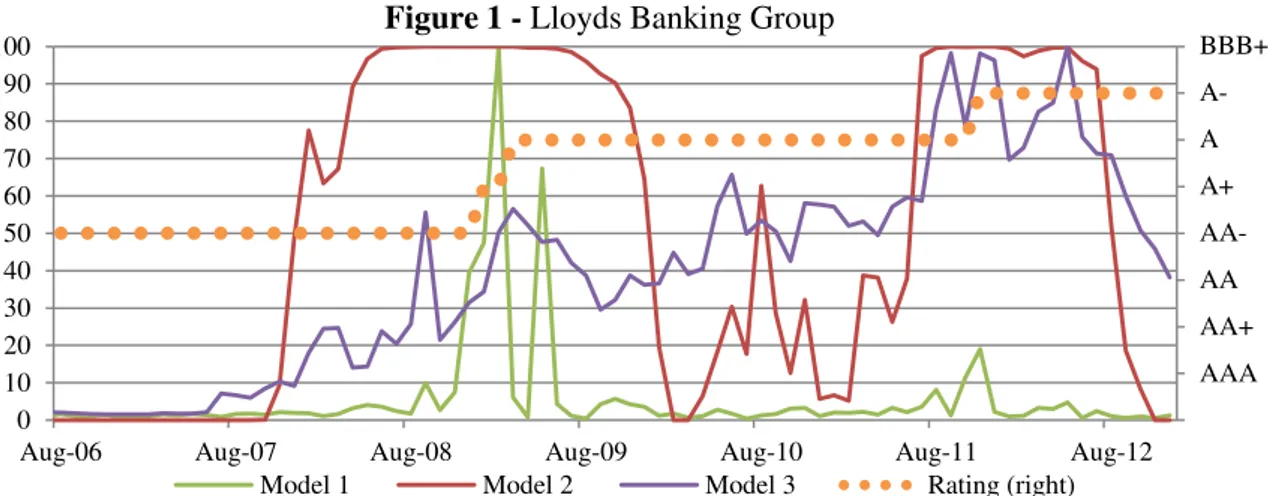
As such, the graphics presented below illustrate the models studied and the credit rating transitions in the period analysed, subject to each company’s available data. Each
model’s credit risk indicator is represented in the left vertical axis and is constrained so
that each model’s maximum corresponds to 100. Therefore, the values depicted do not
represent the “probabilities of default” computed by Models 1 and 2 or the CDS spreads from Model 3; they are just indexes obtained from the original models.
15 Figure 2 below shows the case of Wachovia, which started registering losses in the second quarter of 2008, in the height of the financial crisis. After a turbulent period of losses and with several clients withdrawing money from the institution, Wachovia was forced to be sold, and ended up being acquired by Wells Fargo in 2008. In the graph below one can see Models 2 and 3 signalling a credit risk increase in mid-2007, while Model 1 only shoots after the first downgrade, in July 2008.
From this example it is also relevant to observe that prior to the first downgrade, Wachovia was upgraded twice. In fact, Model 3 suggests an improvement in credit quality, though the decrease in the indicator is much less pronounced than when there is credit risk deterioration. This might suggest that the credit risk indicators analysed are more sensible to credit rating deteriorations than to improvements in the credit quality.
0 1 2 3 4 5 6 7 8 0 10 20 30 40 50 60 70 80 90 100
Aug-06 Aug-07 Aug-08 Aug-09 Aug-10 Aug-11 Aug-12
Figure 1 - Lloyds Banking Group
Model 1 Model 2 Model 3 Rating (right)
0 1 2 3 4 5 6 7 8 9 10 11 0 10 20 30 40 50 60 70 80 90 100
Jan-03 Jan-04 Jan-05 Jan-06 Jan-07 Jan-08 Jan-09
Figure 2 - Wachovia
Model 1 Model 2 Model 3 Rating (right)
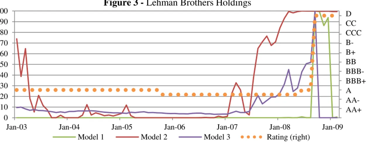
16 Figure 3, presented below, shows the most iconic case of the global financial crisis. In 2008 Lehman Brothers Holdings started registering unprecedented losses and in September 2008 filed for bankruptcy through Chapter 11. Again, Models 2 and 3 start increasing sharply in early 2007, while the first downgrade only takes place in June 2008 and then the firm defaults three months later. As in the previous example, Model 1 only reacts when the company defaults.
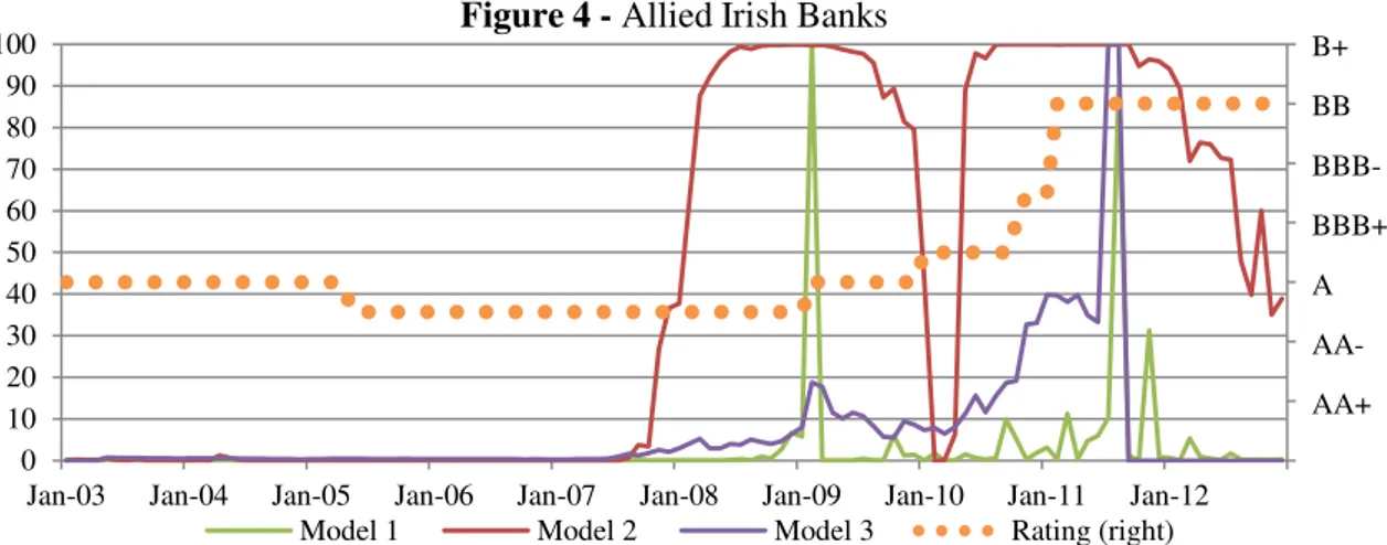
Figure 4 below depicts Allied Irish Banks (AIB), one of the biggest Irish banks that had to be intervened by the Government as a result of the financial crisis. In February 2009 the Irish Government announced a €7 billion rescue package for AIB and then, in December 2010, it had to take a majority stake in the bank. While this bank went into deeper trouble in 2008, Figure 4 shows that the credit risk indicators obtained from Models 2 and 3 start increasing sharply in late 2007, while the first downgrade only takes place in February 2009, when Model 1 registers its maximum.
0 2 4 6 8 10 12 14 16 18 20 22
0 10 20 30 40 50 60 70 80 90 100
Jan-03 Jan-04 Jan-05 Jan-06 Jan-07 Jan-08 Jan-09
Figure 3 - Lehman Brothers Holdings
Model 1 Model 2 Model 3 Rating (right)
17 The graphical analysis performed helps understanding better the behaviour of the credit risk models studied. From the examples presented, one can see that Model 1 only reacts when the credit rating downgrades take place, while Models 2 and 3 start reacting much earlier, suggesting that these models are better to anticipate credit quality deterioration of financial institutions. Nevertheless, it is worth mentioning that, from the graphical analysis, Model 3 appears to be more volatile than Model 2, as in several situations it increases and decreases significantly without any credit rating change happening later; while Model 2 only increases prior to credit rating changes and its increase is much more sustained than that of Model 2. Another relevant remark is that the models are more reactive to credit quality deteriorations than to credit quality improvements, as the variation in the indicators is much less pronounced in this case.
Another important contribution of this work project is that it only includes financial institutions in the sample, contrary to most of the literature on credit risk. For instance, in the studies developed by Bharath and Shumway (2008) and by Das, Hanouna and Sarin (2008), that are referred in this work project, the authors exclude financial firms from their sample. Therefore, this work project concludes that the naïve approach of the Merton (1974) Model and the CDS spreads also analysed by Das, Hanouna, Sarin (2008) are also statistically significant to assess credit risk of financial institutions.
0 2 4 6 8 10 12 14
0 10 20 30 40 50 60 70 80 90 100
Jan-03 Jan-04 Jan-05 Jan-06 Jan-07 Jan-08 Jan-09 Jan-10 Jan-11 Jan-12
Figure 4 - Allied Irish Banks
Model 1 Model 2 Model 3 Rating (right)
B+
BB
BBB-
BBB+
A
AA-
AA+
18 4. Conclusion
The results of this work project provide some interesting, though not unanimous conclusions. From the regressions computed with the three models analysed, it appears that all of them statistically significantly predict credit rating downgrades. However, from the logit multiple regression including the three models, Model 3 appears not to have additional predictive power when combined with Models 1 and 2. On the other hand, from the power curves presented, Model 3 outperforms the other two models.
Nonetheless, it is also important to mention some of the limitations of this study. First, the sample considered only includes large, global banks, where some of them are financial counterparties of the SGFPBP. A sample including smaller banks might have yielded different results. However, the sample was limited to large banks since they have similar characteristics to the financial counterparties of the SGFPBP.
In what concerns Model 1, which, from the graphical examples presented, seems to be the one anticipating downgrades later, it is relevant to mention that when computing the probability of an institution being downgraded in one year, as stated in equation (1),
section 3.1., the explanatory variables’ coefficients ( ) applied were the ones provided by Campbell, Hilscher, & Szilagyi (2006). However, it would be more accurate to estimate these coefficients using the sample of financial firms analysed in this study.
19 Concerning Model 3, this is a much simpler and limitative model, when compared to the previous two, as not all the companies included in the initial sample have CDS contracts or historical data available on their prices, which reduced significantly the observations for this model. Moreover, lack of data was more common in smaller banks (compared to the sample’s median size), which might create a bias regarding firm size.
Overall, the three models studied proved to be significant in predicting credit rating downgrades, and more important, they appear to anticipate credit quality deterioration considerably early, except for Model 1. This suggests the usefulness of these models to monitor credit risk in addition to credit ratings, that instead of anticipating credit risk deterioration, in many situations, companies are only downgraded when the situation is already severe. Notwithstanding, companies all over the world usually rely on these ratings to assess companies’ credit quality and make investment decisions, when other credit risk indicators, such as the ones presented in this study might better and more timely reflect credit risk. A good example of this is that during the 2008 financial crisis several A-rated companies went bankrupt, and credit rating agencies did not anticipate this, while the models presented here did.
20 5. References
Altman, Edward I. 1968. “Financial Ratios, Discriminant Analysis and the Prediction of Corporate Bankruptcy.”The Journal of Finance, 23(4): 589-609.
Altman, Edward I. 2000. “Predicting Financial Distress of Companies: Revisiting the Z-Score and Zeta Models.” http://pages.stern.nyu.edu/~ealtman/Zscores.pdf.
Altman, Edward I., Robert G. Haldeman, and P. Narayanan. 1977. “ZETATM* Analysis – A New Model to Identify Bankruptcy Risk of Corporations”. Journal of Banking & Finance, 1(1): 29-54.
Bharath, Sreedhar T., and Tyler Shumway. 2008. “Forecasting Default with the Merton Distance to Default Model.” The Review of Financial Studies, 21(3): 1339-1369.
Campbell, John Y., Jens Hilscher, and Jan Szilagyi. 2006. “In Search of Distress Risk.” National Bureau of Economic Research Working Paper 12362.
Chava, Sudheer, and Robert A. Jarrow. 2004. “Bankruptcy Prediction with Industry
Effects.” Review of Finance, 8(4): 537-569.
Das, Sanjiv R., Paul Hanouna, and Atulya Sarin, A. 2008. “Accounting-based Versus Market-based Cross-sectional Models of CDS Spreads.” Journal of Banking & Finance, 33(4): 719-730.
Hillegeist, Stephen A., Elizabeth K. Keating, Donald P. Cram, and Kyle G. Lundstedt. 2002. “Assessing the Probability of Bankruptcy.” Review of Accounting Studies, 9(1): 5-34.
Merton, Robert C. 1974. “On the Pricing of Corporate Debt: the Risk Structure of
Interest Rates.” The Journal of Finance, 29(2): 449-470.
O’Kane, Dominic, and Stuart Turnbull. 2003. “Valuation of Credit Default Swaps.”
Fixed Income Quantitative Credit Research – Lehman Brothers.
Ohlson, James A. 1980. “Financial Ratios and the Probabilistic Prediction of
Bankruptcy.” Journal of Accounting Research, 18(1): 109-131.
Saunders, Anthony, and Linda Allen. 2002. Credit Risk Measurement - New Approaches to Value at Risk and Other Paradigms. New York: Wiley Finance. Syversten, Bjørne Dyre H. 2004. Economic Bulletin 4/2004 – “How Accurate are
Credit Risk Models in their Predictions Concerning Norwegian Enterprises?” Norges Bank.
21 6. Appendices
Appendix 1 – Sample of fifty financial institutions used for testing all the models analysed (for Model 3 only the companies identified with “*” were included).
1* HSBC Holdings PLC 26* Deutsche Bank AG
2* Wells Fargo & Co 27 Bank of Montreal
3* JPMorgan Chase & Co 28 Itaú Unibanco Holding SA
4* Bank of America Corp 29* Capital One Financial Corp
5* Citigroup Inc. 30* Bank of China Ltd
6* Commonwealth Bank of Australia 31* Lloyds Banking Group PLC
7 Royal Bank of Canada 32* Sberbank of Russia
8* Westpac Banking Corp 33 Banco Bradesco SA
9* Banco Santander SA 34 Canadian Imperial Bank of Commerce
10 Toronto-Dominion Bank 35 PNC Financial Services Group Inc.
11* Australia & New Zealand Banking Group Ltd 36* Credit Suisse Group AG
12* Mitsubishi UFJ Financial Group Inc. 37 Royal Bank of Scotland Group PLC
13 Bank of Nova Scotia 38* Wachovia Corp
14* Standard Chartered PLC 39 Keycorp
15* US Bancorp 40* Danske Bank A/S
16* National Australia Bank Ltd 41* Svenska Handelsbanken
17* Goldman Sachs Group Inc. 42* Dexia
18 China Construction Bank Corp 43 Comerica Inc.
19* UBS AG 44* Swedbank AB
20* BNP Paribas SA 45 Fifth Third Bancorp
21* Banco Bilbao Vizcaya Argentaria SA 46 National City Corp
22* Barclays PLC 47 SunTrust Banks Inc.
23* Sumitomo Mitsui Financial Group Inc. 48* Lehman Brothers Holdings Inc.
24 ICBC 49* Allied Irish Banks PLC
22 Appendix 2 – Logit regression on 12-months lagged best-model variables, where the dependent variable is failure (binary variable equal to 1 if a firm files for bankruptcy, delists or receives a D rating, and 0 otherwise), according to Campbell, Hilscher, & Szilagyi (2006) paper.
Explanatory Variable (absolute z-statistic) Coefficient
NIMTAAVG
(Profitability)
-20.264 (18.09)
TLMTA
(Leverage) 1.416 (16.23)
EXRETAVG
(Excess Return over S&P500)
-7.129 (14.15)
SIGMA
(Volatility of Stock Returns) 1.411 (16.49)
RSIZE
(Company Market Capitalisation / S&P500 Market Capitalisation) -0.045 (2.09)
CASHMTA
(Liquidity) -2.132 (8.53)
MB
(Market-to-Book Ratio) 0.075 (6.33)
PRICE
(ln of the company’s stock price) -0.058 (1.40)
Constant -9.164 (30.89)
Observations Failures McFadden Pseudo R2
1,565,634 1968 0.114
Appendix 3 – Output for the logit regressions of the downgrade binary variable on the
“probabilities of default” from Models 1 and 2, and the CDS spreads from Model 3.
Explanatory Variable Logit Regressions (Explained Variable: Downgrade Binary)
(1) (2) (3) (4) (5) (6) (7)
Constant -4.2874
(0.0000)* -5.4204 (0.0000)* -4.3179 (0.0000)* -5.3977 (0.0000)* -4.3015 (0.0000)* -5.3998 (0.0000)* -5.3660 (0.0000)*
“Probability of default” –Model 1 4.6319
(0.0000)* - -
2.7209 (0.0001)* 3.7743 (0.0002)* - 3.0740 (0.0017)*
“Probability of default” – Model 2 - 2.8965
(0.0000)* - 2.7565 (0.0000)* - 2.6130 (0.0000)* 2.5756 (0.0000)*
CDS Spread – Model 3 - - 0.0023
(0.0000)* - 0.0020 (0.0000)* 0.0010 (0.0060)* 0.0006 (0.1035)
McFadden R2 0.0341 0.1335 0.0558 0.1476 0.0751 0.1444 0.1593
Adjusted McFadden R2 0.0318 0.1312 0.0526 0.1430 0.0687 0.1380 0.1497
Total Observations 5708 5679 3363 5679 3294 3283 3283
Observations with Dep=1 83 83 63 83 63 63 63
P-values in parentheses
* Coefficients are statistically significant at the 1% significance level
23 Appendix 4 – Correlations matrix for the three models analysed.
Model 1 Model 2 Model 3
Model 1 1.0000 0.1286 0.2895
Model 2 0.1286 1.0000 0.4862
Model 3 0.2895 0.4862 1.0000
Appendix 5 – Power curves for the three models analysed. The Y axis represents the percentage of observations that correspond to a downgrade and that are included in the X% top riskiest observations, from the ranked-by-risk observations of each model.
Appendix 6 – Variables, formulas and respective Bloomberg tickers used to compute all the inputs for Model 1.
Variable Formula Bloomberg Variables and Tickers
Profitability
NET_INCOME -
- Market Value of Total Assets
BS_TOT_LIAB2 CUR_MKT_CAP
Leverage
BS_TOT_LIAB2 -
Liquidity
-
- Cash and Short-Term Assets
BS_CASH_NEAR_CASH_ITEM BS_MKT_SEC_OTHER_ST_INVEST
Market-to-Book Ratio (Directly retrieved from Bloomberg) MARKET_CAPITALIZATION_TO_BV
Log Excess Return Over S&P 500
] PX_LAST
3-Months Standard Deviation (Directly retrieved from Bloomberg) VOLATILITY_90D
Market Capitalisation vs. S&P 500 (
) CUR_MKT_CAP
Log of Stock Price PX_LAST
0% 20% 40% 60% 80% 100%
0% 20% 40% 60% 80% 100%
24 Appendix 7 – Variables, formulas and respective Bloomberg tickers used to compute all the inputs for Model 2.
Variable Formula Bloomberg Variables and Tickers
Market Value of Debt (naïve )
-
- Current Liabilities
BS_ST_BORROW BS_OTHER_ST_LIAB
- Long-Term Debt
BS_LT_BORROW BS_OTHER_LT_LIABILITIES
Volatility of Debt ( )
- Equity Volatility ( )
√ PX_LAST
Total Volatility of the Firm ( )
-
- Equity (Directly retrieved from Bloomberg) CUR_MKT_CAP
Return on Firm’s Assets ∏
PX_LAST
Distance to Default ( ) ( )
√ -
Probability of Default -
Appendix 8 – Bloomberg description of all the variables used to compute the inputs for Models 1 and 2, mentioned in Appendices 7 and 8; for the CDS spreads from Model 3; and for the credit rating transitions assigned by the S&P rating agency.
Bloomberg Ticker Bloomberg Description
NET_INCOME
Net Income (Losses) The profits after all expenses have been deducted.
BS_TOT_LIAB2 Total Liabilities
= Customers' Acceptances and Liabilities + Total Deposits + ST Borrowings + Other ST Borrowings + Securities Sold with Repurchase Agreements + LT Borrowings + Other LT Liabilities
CUR_MKT_CAP Total Current Market Value
Total current market value of all of a company's outstanding shares stated in the pricing currency.
BS_CASH_NEAR_CASH_ITEM Cash and Near Cash
Includes cash in vaults and non-interest earning deposits in banks. Includes receivables from the central bank and postal accounts. Includes cash items in the process of collection and unposted debits. Interest bearing deposits in other banks are included in interbank assets. Includes statutory deposits with the central bank.
BS_MKT_SEC_OTHER_ST_INVEST Marketable Securities and Other Short-Term Investments
Includes trading securities and securities held for sale. Includes loans and mortgage-backed securities held for sale. Includes treasury bills.
May include short-term interest-bearing loans to third parties if not disclosed separately. If disclosed separately, such loans are classified in Other Current Assets.
Includes holdings of gold and silver.
25 Appendix 8 – Bloomberg description of all the variables used to compute the inputs for Models 1 and 2, mentioned in Appendices 7 and 8; for the CDS spreads from Model 3; and for the credit rating transitions assigned by the S&P rating agency.
Bloomberg Ticker Bloomberg Description
MARKET_CAPITALIZATION_TO_BV
Market Capitalisation to Book Value Measure of the relative value of a company compared to its market value.
PX_LAST Security Last Price
Equities: Returns the last price provided by the exchange.
Equity Indices: Returns either the current quote price of the index or the last available close price of the index.
VOLATILITY_90D 90-Days Volatility
Measure of the risk of price moves for a security calculated from the standard deviation of day to day logarithmic historical price changes. The 90-day price volatility equals the annualized standard deviation of the relative price change for the 90 most recent trading days closing price, expressed as a percentage.
BS_ST_BORROW Short-Term Borrowings
Includes bank overdrafts, short-term debts and borrowings, repurchase agreements (repos) and reverse repos, short-term portion of long-term borrowings, current obligations under capital (finance) leases, current portion of hire purchase creditors, trust receipts, bills payable, bills of exchange, bankers acceptances, interest bearing loans, and short term mandatory redeemable preferred stock. Net with unamortized premium or discount on debt and may include fair value adjustments of embedded derivatives.
For banks and financials, includes call money, bills discounted, federal funds purchased, and due to other banks or financial institutions.
BS_OTHER_ST_LIAB Other Short-Term Liabilities
Other current liabilities that do not bear explicit interest such as accrued expenses, accrued interest payable.
Includes the liability side of customers' acceptance liabilities. Includes fair value adjustments to derivatives and insurance policies.
BS_LT_BORROW Long-Term Borrowings
All interest-bearing financial obligations that are not due within a year.
Includes convertible, redeemable, retractable debentures, bonds, loans, mortgage debts, sinking funds, and long-term bank overdrafts.
Excludes short-term portion of long term debt, pension obligations, deferred tax liabilities and preferred equity.
Includes subordinated capital notes.
Includes long term hire purchase and finance lease obligations. Includes long term bills of exchange and bankers acceptances.
May include shares issued by subsidiaries if the group has an obligation to transfer economic benefits in connection with these shares.
Includes mandatory redeemable preferred and trust preferred securities in accordance with FASB 150 effective June 2003.
Includes other debt which is interest bearing. Net with unamortized premium or discount on debt. May include fair value adjustments of embedded derivatives.
BS_OTHER_LT_LIABILITIES Other Long-Term Liabilities
This field includes all other long-term obligations that do not bear explicit interest. Includes provision for charges and liabilities, pension liabilities, retirement allowance accounts, deferred tax liabilities, and discretionary reserves.
Long-term pension assets disclosed as a negative on the liability side are netted with Other LT liabilities.
Includes provision for general banking risks.Includes insurance reserves for banks that are also active in the insurance sector.
PX_ASK
Last Price Lowest price a dealer will accept to sell a security.
RTG_SP_LT_FC_ISSUER_CREDIT