THE STEERING TOOL OF FINANCIAL INSTITUTIONS:
CREDIT VAR (VALUE AT RISK)
B RBULESCUăMARINELA
,
LECTURER PH.D., UNIVERSITY OF PITESTI, PITESTI, ROMANIA
,
e-mail:
[email protected]
HAGIU ALINA,
LECTURER PH.D., UNIVERSITY OF PITESTI, PITESTI, ROMANIA,
e-mail:
[email protected]
VASILI
C
RADU,
LECTURER PH.D., UNIVERSITY OF PITESTI, PITESTI, ROMANIA,
e-mail:
[email protected]
Abstract
In order to determine the economic capital, in terms of internal management or of application of regulations, financial institutions need to model the probability of future losses on a loan portfolio. This is generally made applying the Credit VaR method. Thus, unexpected losses can be assessed.
Key Words: value at risc, economic capital, market risc, credit portofolio.
JEL Classification: G32
Introduction
In order to determine the economic capital, in terms of internal management or of application of regulations, financial institutions need to model the probability of future losses on a loan portfolio. This is generally made applying the Credit VaR method. Thus, unexpected losses can be assessed.
1.
Data concerning the notion of Value-at-Risk
After the resounding bankruptcy of several large financial institutions (Metallgesellschaft – loses more than 1.5 billion dollars from oil futures market transactions (1993); Barings – the oldest British bank, at that time, lost more than 1.3 billion dollars (1995), Sumito Bank) [1], the international bank authorities set themselves to establish strict risk monitoring rules. Indeed, the increased volatility in the financial markets and the wide variety of complex financial tools held in the portfolio generated the need to have a synthetic indicator of the market risk incurred.
The Value-at-Risk methods tend to answer this need. Market risk is defined as the risk of potential losses on balance sheet items and off-balance sheet as a result of market price variations. It covers the risks concerning instruments related to the interest levels, instruments related to titles of ownership (Shares) and the risk of change. Rarely, an instrument such as VaR was so quickly adopted by the entire international financial community.
The Value-at-Risk is defined as the potential loss a financial institution can suffer during a defined period of time (holding horizon) and a high probability level (confidence interval). It can be measured at global level or at the scale of a certain portfolio. Therefore, it is possible to know precisely the positions that generate risk. Moreover, the selection of the parameters allows for defining a strategy related to risk.
Prudence is expressed by determining three parameters in an intelligible manner: the holding horizon, the level of risk and the VaR limit. The holding horizon depends on the nature of the portfolio. It is supposed to be associated to the sequence of liquidation of the portfolio on the market. In relation to the probability level, it reflects the aversion for the risk of the considered.
Generally, VaR is calculated under the assumption that the markets operate normally (extreme conditions such as a crash are not taken into account. It is also a manner of developing a common language in relation to risk. Moreover, it allows for turning the risky nature of a balance sheet item into a capital measure necessary to cope with that risk.
Or the probability of a value lower than W* is equal to 1-c=p :
This specification is valid for any distribution and does not allow, at any moment, the intervention of the notion of standard deviation, but only that of quantile. Traditionally, it is assumed that the yields and Gaussian. In this case, the calculation of VaR is very much simplified. Indeed, the VaR figure can be deduced directly from the standard deviation of the asset (or of the portfolio) using a multiplicative factor dependent on the confidence level. The calculation of the VaR is thus made by calculating W* in such a way as the area at its left is equal to 1-c, which is given by a table opposite compared to the normal law. Thus, for a normal distribution and a short horizon, (since the average is null), the standard deviation of the distribution on the horizon taken into account a is :
Therefore, the position of the tail of distribution to the left can be calculated at (1-c) %.
Where:
σ= volatility of the asset considered ∆ = number of assets in the portfolio
δt = without time depending on the selected horizon
α (1- c) = reverse function of the normal density depending on the confidence level
W* = lowest value (quantile) that can be achieved by the portfolio at the time horizon, corresponding to the selected confidence level;
VaR is a quantile of the distribution of the profitability, with the property that, with a low probability, the loss will be lower than the VaR figure on a determined time horizon.
2.
Requirements of the National Bank of Romania concerning the Var reporting
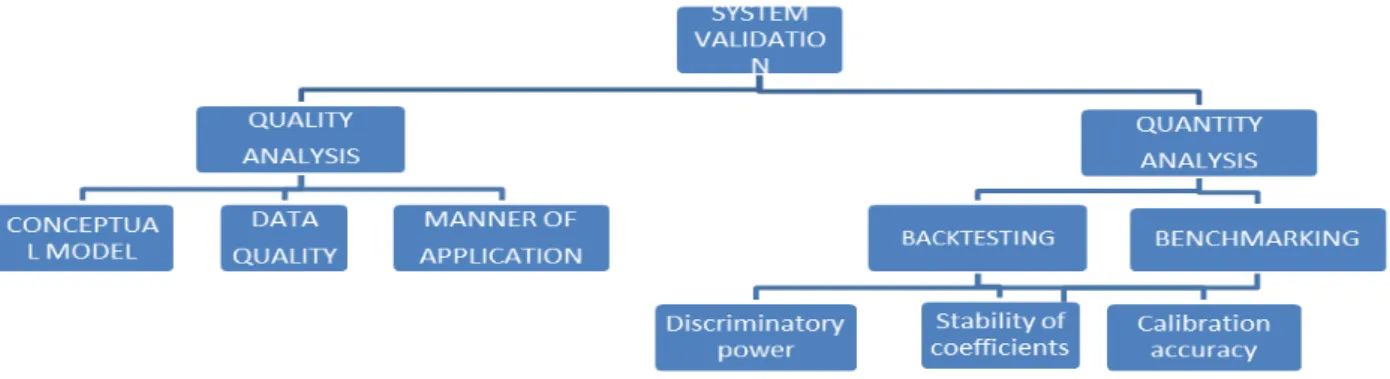
As part of the assessment of the exposure to the market risk, banks shall report own measures of the exposure to the market risk under the form of information supplied by the VaR systems at the level of the trading book. The reporting will include both quality and quantity information.[1]
The set of quantity information comprises a short description of the VaR system, as follows:
Types of VaR models used (variance/covariance, historical simulation, Monte Carlo simulation, etc.)
The technique of assessment of the variance/covariance (simple moving average, weighted moving average, Garch, etc.)
Description of the procedures of aggregation of the VaR measures between various risk factors Description of the procedures of allocating and monitoring the VaR limits
Description of the validation and testing techniques (backtesting) of the model Other specifications
The set of quantity information includes:
The values of VaR at the reporting time, as well as the minimum/medium/maximum values recorded in the previous quarter;
VaR limits at the Trading Book level (aggregated limit, risk factor limits – interest rate/exchange rate); Results of the back testing of the VaR system.
According to the regulations of the National Bank of Romania, VaR reporting will be the result of systems that will be in compliance with a minimum set of quantity standards, including:
The minimum holding period will be 10 days. VaR will be assessed daily.
The confidence margin for the VaR measures will be 99%.
The backtesting will be made on a horizon of at least 250 days.
Figure 1Quality and quantity aspects of the validation process
Source: Armeanu D., Bãlu F., Aplicarea metodologiei VaR portofoliilor valutare deținute de bănci, pg.87
http://store.ectap.ro/articole/197.pdf
3.
Case Study
For example, a VaR at 10 days for a confidence interval of 99% equal to 1 million Euros means that, if the portfolio is held for 10 days, then there are 99% chances of not losing more than 1 million Euros in 10 days, but there are also1% chances of losing 1 million Euros in the following days. VaR does not allow us, in any way, to know what we can lose in the worst case scenario.
VaR application in the case of credit risk
Banking and financial institutions must put in place a management of the credit risk they bear. Nevertheless, as described hereinabove, it has several characteristics that limit their treatment.
Review of the credit risk specificities
Credit risk is present at two main types of borrowers
Issuer risk is the credit risk (lack of quality or degradation thereof) concerning a cash financial instrument, such as an bond or a bank loan. It exposes the lender to a loss if it cannot cover the entire amount due for the contract.
The counterparty risk is the credit risk related to the counterparty of a non-financed instrument such as a swap, an option or a guarantee.
Generally, as indicated hereinabove, credit risk is evaluated through the amount corresponding to the debt or the commitments on the debtor (the “exposure” multiplied by the error probability of the latter at the commitment horizon. The result is readjusted for the hope to recover the assets after the emergence of the error. On the other hand, it is measured in a different manner in relation to the issuer risk and the counterparty risk:
For the “cash” products, credit risk is calculated in relation to the amount borrowed, to which interests are added;
For derivative products, the credit risk is calculated on the market value of the item (“mark-to-monkey” for the products negotiated on an organised market, or “mark-to-model” for the products negotiated in contracts).
The coverage risk is related to several factors :
For the issuer risk, the recovery level depends on how old is the debt to which the creditor is exposed, in other words, its priority level related to cash flows in case of liquidation by the court;
For the issuer and counterparty risk, it depends on the existence or absence of the collaterals, and on the debtor’s nature (the coverage levels vary depending on the size of the latter, its country of origin, its field of activity, etc).
It is a systemic risk. It is influenced by the general context, therefore it is cyclic and closely related to the economic activity (increases during the depression periods and decreases during the growth periods). Financing the economy and the present increase of the pro-cyclical characteristics. Banks are willing to finance the economy when “everything goes well”, but try to withdraw in times of recession. It originates, among others, in the inherent financial instability of a financial system globalized and liberalized due to the absence of adjustment through prices: a credit oversupply does not imply a decrease in prices (on the contrary!).
Moreover, it is a specific risk : it evolves depending on the events specific to the borrowers. Credit risk related to an issuer or a counterparty is directly influenced by intrinsic characteristics: its size, the evolution of its economic environment, the events that affect it, etc.
Finally, credit risk has an asymmetric profitability structure (as opposed to other risks). It is characterised by a profitability profile different from other risks due to its connection to the borrower’s individual performance and financial structure. Indeed, while market risk s symmetric and can be approached through a normal law, credit risk manifests “fat tails” phenomena and a certain skewness. The lender has a high probability to earn a small gain (interests charged in relation to the debt) and a low probability to lose big part of its original stake. This has significant consequences for the modelling.
Credit VaR implementation
Credit VaR is the initial loss of a credit portfolio for a given statistic confidence interval, on a defined time horizon (generally one year) due to credit risk. Contrary to market risks which are valued daily, Credit VaR is a quantile of the distribution of the credit portfolio losses, not a quantile of the distribution of the relative variations at the value of the assets in the portfolio. The portfolio losses are modelled based on the knowledge of the individual risks and on the dependences of the losses [4]. Thus, calculating a Credit VaR implies calculating the variations of the negative values of the credit portfolio on a given time horizon (the holding period) taking into account the credit risk. The purpose is to determine the influence of the risk of changing the credit scoring on the value of the portfolio.
It is probably convenient to determine the law of distributing the change of the portfolio value, which can be used to calculate the VaR. Regardless of the technique retained to calculate Credit VaR (empirical or parametric), it follows a three-step process:
Determining the transition probabilities between t=0 and the holding period retained from one rating to another;
Calculating the value of the products in the portfolio at the horizon taken into account for each rating possible;
Determining a histogram of then overall value of the portfolio, built by means of dependences (linear correlation under the assumption of multivariate normality).
The empirical Credit VaR is determined by “reading” directly into the distribution of losses.
This approach has certain limitations: first of all, its poor predictive nature, due to the fact that all the data used are historical data; nevertheless, in finance, it has long been established that the past does not allow for the elaboration of predictions related to the future. On the other hand, the transition matrices used are unstable and ratings do not vary continuously. Finally, the empirical VaR is not sub-additive, so it does not take into account the effects of diversification; and even worse, it will not be supra-additive.
Example of calculation of Credit VaR for an isolated asset, using the transition matrices provided by the rating agencies and which are based on the valuation of the assets by update resorting to the forward rate curve.
If we have a bond with a value of 100 Euros, with a 3-year residual maturity, paying a coupon rate of 6% per year (the next one will be paid in a year), whose issuer’s rating is A. For simplification reasons, only 5 ratings will be taken into account. The structure based on notions such as the forward rate is known nowadays for each rating starting with the cash rates.
Table 1: Example of calculation of Credit VaR for an isolated asset
Ratings Forward rate in a year from one year
Forward rate in a year from 2 years AAA A BBB CCC 5% 5.06% 5.60% 15.50% 5.01% 5.15% 6.20% 18.50%
D Recovery rate
= 40% of the nominal value
The time horizon retained is 1 year. In one year, after increasing the coupon of the bond price, unless the issuer changes the rating, will be :
P (in the case of rating A)=6/1.0506+106/(1.0515)2=101.58
P (in the case of rating AAA)=6/1,05+106/(1,0501)2=101,84
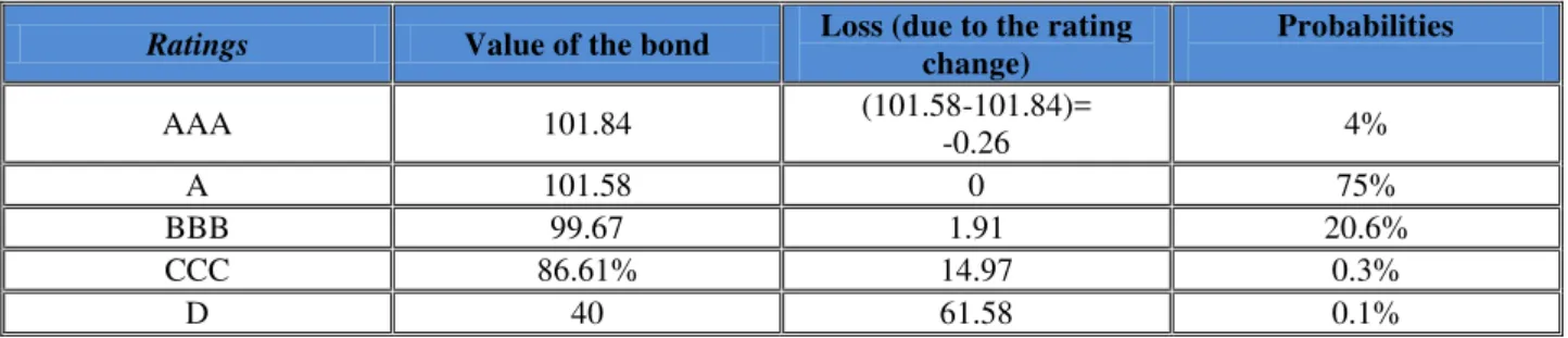
The possible values of the bond in one year are calculated here taking into account the change of the rating and integrating the transition matrix which contains the probabilities of the rating change.
Thus we can build the potential loss distribution function:
Table 2: The possible values of the bond in one year
Ratings Value of the bond Loss (due to the rating change)
Probabilities
AAA 101.84 (101.58-101.84)=
-0.26 4%
A 101.58 0 75%
BBB 99.67 1.91 20.6%
CCC 86.61% 14.97 0.3%
D 40 61.58 0.1%
Therefore, the empirical distribution function is:
Table 3: The empirical distribution function
Losses Probabilities Cumulated probabilities
-61,58 0.1% 0.1%
-14,97 0.3% 0.4%
-1,91 20.6% 21%
0 75% 96%
+0,26 4% 100%
In this example, there are 99.6 % chances not to lose more than 14.97 Euros in the next year, which also means that there are 0.4% chances to lose more than 14.97 Euros. Credit VaR (like Market VaR) does not say anything about what you can lose in the worst case scenario.
In these calculations, the assumption is that only credit risk is responsible for the bond price variations. The risk corresponding to the interest rate (market risk) is not integrated insofar as the forward rates used are determined at the moment of the calculation.
Consequently, starting from Credit VaR, a financial institution can calculate the level of the equity able to absorb extreme losses.
Therefore, Credit VaR allows for the assessment of the potential loss that can be borne by the institution at an increased probability level for the given horizon. It is located in a very conservative area, taking into account what could happen in the worst case scenario. This extreme loss allows for the calculation of the equity amount required to cover these extreme risks. In order to measure the potential loss at a given horizon, it is necessary to know the distribution of the probable losses. Starting from this function, the potential losses are determined.
In other words, we will measure the Credit VaR of the credit portfolio selecting the distribution quantile. The economic equity (or the economic capital) required to cover these losses will be assessed as follows: the value of the unexpected losses corresponds to the distance between Credit VaR and the average loss. Therefore, the capital requirement is thus obtained adding expected losses and unexpected losses. Este important to mention that Credit VaR is just a limited instrument when it comes to measuring unexpected losses. This tool has a number of indirect means which depend on the assessment technique used (empirical, parametric).
Bibliography
[1]Armeanu D., Bãlu F., „Aplicarea metodologiei VaR portofoliilor valutare deținute de bănci”, http://store.ectap.ro/articole/197.pdf;
[3]Hoggarth G., Logan A., Zicchino L., „Macro Stress Tests of UK Banks”, Manuscript, Bank of England, 2004, http://www.bis.org/publ/bppdf/bispap22t.pdf;
[4]Kharoubi C.,Thomas P., „Analyse du risque de crédit”, RB Edition, Paris, 2013;
[5]Roșoag A., „Utilizarea metodologiei Value-at-Risk în gestiunea riscului și optimizarea portofoliilor”, http://www.sorec.ro/pdf/OEcoN3/12_A.Rosoaga.pdf;
[6]Sorge M., „Stress-Testing Financial Systems: An Overview of Current Methodologie”, Working paper no.165, Monetary and Economic Department, Bank for International Settlements, 2004 http://www.bis.org/publ/work165.htm; [7]Tomiț T., „Valoarea la Risc Value at Risk (VaR)”, BRM Business Consulting, http://www.riskmanagement.ro