MEASUREMENT OF ETHANOL SUBSIDIES AND
ASSOCIATED ECONOMIC DISTORTIONS: AN
ANALYSIS OF BRAZILIAN AND U.S. POLICIES
Mario de Queiroz Monteiro Jales* Cinthia Cabral da Costa†
Resumo
Este estudo tem por objetivos medir os valores dos subsídios equiva-lentes das políticas de apoio ao etanol nos Estados Unidos e no Brasil e estimar a magnitude das distorções econômicas por eles causadas. Para o período entre 2002 e 2011, os valores anuais médios destes subsídios fo-ram de US$7,2 bilhões nos Estados Unidos e US$2,1 bilhões no Brasil. As políticas brasileiras elevaram o preço mundial em média em 2,7% neste período, elevando a produção nos dois países (1,2% nos Estados Unidos e 5,3% no Brasil), reduzindo o consumo norte-americano em 4,7% e ex-pandindo o consumo brasileiro em 16,1%. Já as políticas dos Estados Uni-dos deprimiram o preço mundial em média em 2,4% no mesmo período, expandindo o consumo nos dois países (2,5% no Estados Unidos e 1,3% no Brasil), aumentando a produção norte-americana em 8,3%, mas provo-cando uma queda de 4,7% na produção brasileira. Em 2012, ambos países mudaram suas políticas, mas as distorções no mercado permanecem.
Palavras-chave:Etanol; Subsídio; Tarifa de importação; Biocombustíveis. Abstract
The objectives of this study were to measure the subsidy equivalent value of ethanol policies in the United States and Brazil, and estimate the magnitude of associated economic distortions. For 2002-11, average an-nual ethanol subsidy levels were US$7.2 billion in the United States and US$2.1 billion in Brazil. Brazilian support measures for ethanol increased the world price by 2.7% on average in this period, which expanded output in both countries (1.2% in the United States and 5.3% in Brazil), reduced U.S. consumption by 4.7% and increased Brazilian consumption by 16.1%. On the other hand, U.S. ethanol policies depressed world prices by 2.4% on average in the same period, which boosted consumption in both coun-tries (by 2.5% in the United States and 1.3% in Brazil), expanded U.S. pro-duction by 8.3%, but reduced Brazilian output by 4.7%. Although both countries changed their policies in 2012, distortions remain.
Keywords:Ethanol; Subsidy; Import tariff; Biofuels.
JEL classification:F13, Q17, Q18, Q41, Q42, Q48.
DOI:http://dx.doi.org/10.1590/1413-8050/ea375
*Ph.D., Charles H. Dyson School of Applied Economics and Management, Cornell University.
E-mail: [email protected]
†Researcher at Embrapa. E-mail: [email protected]
1
Introduction
Alternative transportation fuels with a lower carbon imprint have been at the center of the debate on global warming and the need to mitigate atmospheric concentrations of greenhouse gases. Biofuels stand out in this discussion for their renewable nature and potential to reduce carbon dioxide equivalent emissions. As a number of countries have adopted policies to encourage the development of biofuel markets, biofuel use has expanded significantly in re-cent years. World consumption of fuel ethanol, the most widely used biofuel, increased from 20 billion liters in 2002 to 80 billion liters in 2012 (LMC 2013). The United States and Brazil, the world’s largest producers and consumers of fuel ethanol, accounted for approximately 85% of global production and con-sumption in 2012 (LMC 2013). The ethanol market support policies adopted in these two countries have significantly impacted producers or consumers of motor fuels.
This study has two main objectives. First, to assess the subsidy equiva-lent value of policies that affect ethanol supply and demand in Brazil and
the United States. Second, to estimate the size of the distortions caused by these policies. The concept of subsidy equivalent corresponds to the mone-tary value of all transfers from consumers and taxpayers that affect
produc-tion, consumpproduc-tion, income, trade or the environment. This measure is based on the indicators of support used by the Organization for Economic Coop-eration and Development (OECD) to monitor and evaluate developments in agricultural policy, establish a common basis for policy dialogue among coun-tries, and provide economic data to assess the effectiveness and efficiency of
policies (OECD 2008). The study focuses on the period following the deregu-lation of the Brazilian sugarcane industry (2002-12).
This paper is divided into four sections in addition to this introduction. Section 2 analyzes U.S. and Brazilian policies that affect the ethanol sector
and develops a methodology to estimate the monetary value of these mea-sures. Section 3 discusses subsidy equivalent estimates for the two countries under analysis. Section 4 assesses the magnitude of the market distortions caused by U.S. and Brazilian ethanol policies. It evaluates the impact of sup-port measures on ethanol prices, supply and demand in the United States and Brazil. Finally, Section 5 draws conclusions and addresses the implications of past and current policies.
2
U.S. and Brazilian ethanol policies
This section develops a theoretical model to estimate the subsidy equivalent value of U.S. and Brazilian public policy measures that support their respec-tive ethanol sectors. Brazilian policies for hydrous and anhydrous ethanol are examined separately.
2.1 U.S. ethanol policies
four main policy instruments in 2002-12: (i) subsidies on feedstock used in the production of ethanol (mainly corn); (ii) a tax credit for blended ethanol; (iii) a mandate establishing a minimum volume of renewable fuel that must be blended with conventional transportation fuels sold or offered for sale in
the United States, and (iv) tariffs and other charges on imported ethanol.1
These measures were not always consistent with declared U.S. biofuel policy goals. For example, while the import tariffon ethanol supported U.S. farmers’
income, it did not contribute to the reduction of greenhouse gas emissions, as it barred the entry of foreign sugarcane ethanol, which has a lower carbon imprint than domestic ethanol produced from corn.
Figure 1 represents corn supply and demand curves in the United States. The shaded area delimited by the rectangleabcdidentifies the total subsidy on domestic corn production (Guscorn); the areaaefdidentifies the portion of this
total subsidy that corresponds to the corn used in ethanol production (Gus1 ).
Notes:Guscornis the total value of corn production subsidies in the United States;Gus1 is
the portion of total corn subsidies that directly benefits the U.S. ethanol sector;gcornus is the unit value of U.S. corn subsidies;Pus
cornis the U.S. domestic price of corn;Ycornus is the volume of corn produced in the United States;Ycornus
→ethanolis the volume of corn used in the production of ethanol in the United States;Dcornis corn demand;Dcorn→ethanol is demand for corn to produce ethanol;Scornand is corn supply.
Source: Authors.
Figure 1: Supply and demand curves for corn in the U.S. and
correspond-ing subsidy equivalent measures
The contribution of corn production subsidies to the ethanol production chain is obtained by multiplying the value of total corn subsidies by the frac-tion of total domestic corn producfrac-tion that is used in ethanol producfrac-tion. Al-gebraically, this is given by equation 1. The data required to estimateGus1 are presented in Table 1.
Gus1 =Guscorn∗
Ycornus →ethanol Ycornus
!
(1)
The mandate and the tax credit increase the demand for ethanol and lead to higher ethanol domestic prices. On the other hand, border barriers ensure a domestic price above the international price and reduce the demand for
1In addition, state governments provided a combination of subsidies, producer incentives
ethanol. The blender — an intermediary between the producer and the end consumer — mixes ethanol and gasoline in a proportion established in the mandate and distributes the blended fuel to filling stations. The ethanol that the blender adds to gasoline was eligible for either a tax exemption or a tax credit until 2011.2 The value of the tax exemption/credit was US$0.54 per
gallon between 1990 and 2004, US$0.51 per gallon between 2005 and early 2009, and US$0.45 per gallon between 2009 and 2011. In order to prevent foreign producers from benefiting from this tax credit, the United States ap-plied an import charge of US$0.54 per gallon of ethanol,3 in addition to an ad valoremimport tariffof 2.5% of the import value. While the tax credit and
the specific import charge were eliminated in 2012, but thead valoremimport tariffremained in place.
Table 1: U.S. subsidies to corn used in ethanol production, 2002-12
Year Cornproduction (Yus
com)
Corn used in ethanol production (Yus
com→ethanol)
Domestic support to corn production (Gus
com)
Ethanol production from corn (Yus)
Ethanol CIF import unit value (Pus
imp)
Million tons Million tons Million US$ Million liters US$/liter
2002 227.7 25.3 2,498 8,102 0.36
2003 256.2 29.6 3,440 10,617 0.30
2004 299.9 33.6 5,309 12,888 0.32
2005 282.3 40.7 10,139 14,781 0.46
2006 267.6 53.8 5,797 18,491 0.63
2007 332.1 77.5 3,806 24,687 0.55
2008 307.4 93.4 4,194 35,240 0.62
2009 333.0 116.0 3,779 41,407 0.56
2010 316.2 127.5 3,495 50,342 0.75
2011 313.9 127.3 4,634 52,805 0.85
2012 272.4 114.3 2,702 47,420 0.78
Sources: Fapri (2013), USDA (2013a,b), USITC (2013), WTO (2013).
By itself, the blenders’ tax credit may not benefit domestic ethanol produc-ers. If the tax credit resulted in a lower final price for blended fuel, this would increase the demand for both ethanol and gasoline, since the final product in the U.S. market is a blend of both fuels. The imposition of the import charge on ethanol prevents this from happening as it raises the domestic price of ethanol and ensures a producer price that is higher than the import price. It is the import charge, and not the tax creditper se, that assists ethanol domestic production.
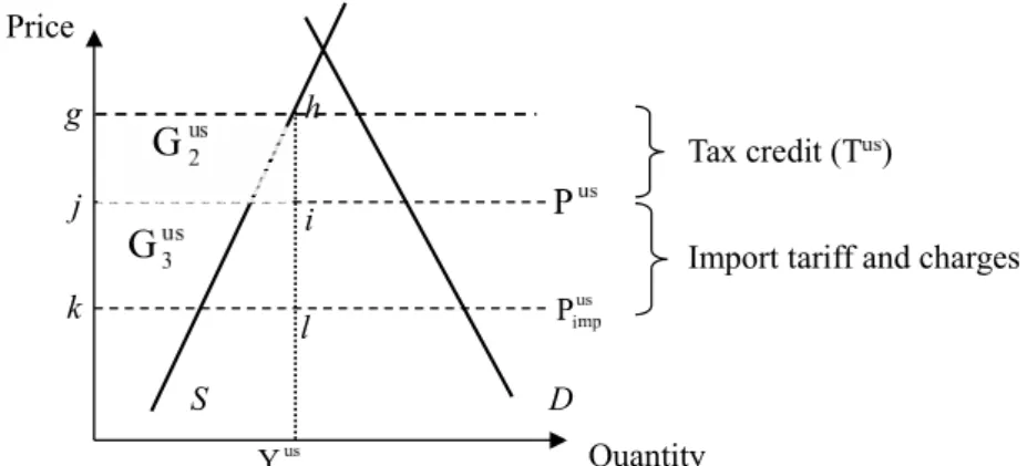
The subsidy equivalent value derived from the tax credit (Gus2 ) corresponds to the product of the tax credit unit value (Tus) and domestic ethanol produc-tion volume (Yus). This is illustrated in Figure 2 by the areaghijand expressed algebraically by equation 2:
G2us=Yus∗Tus (2)
For the years in which the United States was a net importer of ethanol (2002-2009), the subsidy equivalent value derived from import barriers
corre-2The American Jobs Creation Act of 2004 changed the mechanism of the ethanol subsidy
from an excise tax exemption to a blender tax credit (Tyner 2008).
sponds to the product of the total volume of ethanol produced in the United States and the difference between the domestic price and the price of imported
ethanol. This value is illustrated in Figure 2 by the areaijkland is expressed
algebraically by equation 3:
Gus3 =Yus∗(Pus−Pimpus ) (3)
The blending mandate is incorporated in the model only through the vol-ume of ethanol produced domestically. This policy increases demand and helps determine the volume of ethanol produced in the United States. The total value of U.S. subsidies to the ethanol production chain (Gus) is given by
the sum of the areas defined byadfein Figure 1 andghijandijklin Figure 2.
Algebraically, it corresponds to the sum ofGus1 ,G2usandGus3 .
Notes:Gus2 andGus3 are the subsidy equivalent values for ethanol production;Yusis the volume of ethanol produced domestically;Pusis the domestic price of ethanol; and Pimpus is the ethanol import price to the United States.Dis demand andSis supply. Source: Authors.
Figure 2: Supply and demand curves for U.S. ethanol market and corre-sponding subsidy equivalent measures
2.2 Brazilian hydrous ethanol policies
There are two types of ethanol used as transportation fuel in Brazil: (i) anhy-drous ethanol, which is blended into gasoline; and (ii) hyanhy-drous ethanol, which is used alone in automobiles with specially designed engines. In this context, Brazil’s support to the ethanol industry had three main components in the period analyzed: (i) a mandatory blending of anhydrous ethanol into gaso-line, (ii) a lower tax rate for hydrous ethanol than for gasoline (i.e.differential
tax rate), and (iii) another policy that, recently, has had a great effect on the
ethanol market is the control exerted by the Brazilian government over the price of gasoline. Since most Brazilian producers can switch production be-tween the two types of ethanol, the differential tax rate on hydrous ethanol
also indirectly impacts anhydrous ethanol production.
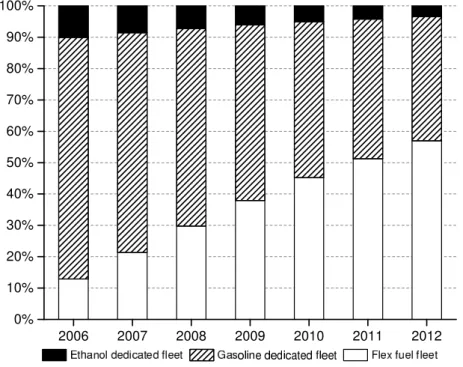
The first commercial flexible fuel vehicle capable of running on any blend of gasoline and ethanol was launched in early 2003. Since then, flexible fuel cars have led sales of new automobiles and have rapidly changed the profile of Brazil’s automobile fleet. Figure 3 illustrates the change in the composition of the fleet, by fuel type, between 2003 and 2012.
The competition between gasoline and hydrous ethanol in Brazil has inten-sified with the growth in the fleet of flexible fuel automobiles (Costa & Guil-hoto (2011)). However, some competition between these two fuels already existed prior to the advent of flexible fuel engines, as they were preceded by engines that ran exclusively on hydrous ethanol.4 From the 1980s until 2003,
Brazilian consumers chose between gasoline and hydrous ethanol when they decided on the type of automobile to buy at the dealer. Since 2003, Brazilians, who have flex fuel vehicles, have been able to choose between gasoline and hydrous ethanol every time they fill up at the pump.
Source: UNICA (2013b).
Figure 3: Brazilian fleet of vehicles (Otto cycle), by fuel type, 2006-12
After the deregulation of the Brazilian sugar-ethanol sector in the late 1990s, the federal government has stimulated the consumption of hydrous ethanol at the expense ofgasoline C (a mixture of 75-80% gasoline and 20-25% anhydrous ethanol) through the difference in final price paid by the
con-sumer. This policy is implemented by the imposition of a higher tax burden on gasoline C as compared to hydrous ethanol.
There are four main taxes on transportation fuels in Brazil: (i) the Contri-bution from the Intervention on the Economic Domain (CIDE), (ii) the
tribution to the Program of Social Integration (PIS), (iii) the Contribution to the Financing of Social Security (COFINS), and (iv) the Tax on the Circula-tion of Goods and Services (ICMS). While the first three are federal taxes, the third is a state tax. Given the weight of the ICMS, the overall tax burden must be calculated individually for each state. Furthermore, while the CIDE tax is payable only on gasoline C, the PIS, COFINS and ICMS taxes are payable on both gasoline C and hydrous ethanol.
The CIDE tax rate was R$0.28 per liter in 2002-07, R$0.18 per liter in 2008, R$0.23 per liter in 2009-10, R$0.15 per liter in 2011, and R$0.09 per liter between January and June 2012, when it was finally eliminated (Brazil-ian Ministry of Finance (2013)). The PIS/COFINS tax rate remained around 9.25% in the period 2002-12. The prices of transportation fuels and the ICMS tax rates differ from state to state. Average ICMS rates5and consumption
lev-els for ethanol and gasoline in each Brazilian state in 2002-12 are shown in Figures 4 and 5.
A third Brazilian policy that affects ethanol markets consists of
government-controlled gasoline prices. Figure 6 shows the difference between annual
av-erage domestic and international gasoline prices between 2002 and 2012. Do-mestic prices were moderately higher than international prices between 2002 and 2009. This difference became more significant in 2010, when domestic
prices were on average 30% higher than international prices, encouraging the consumption of hydrous ethanol in place of fossil fuels. The opposite oc-curred in 2012, when domestic gasoline prices were substantially lower than world prices, discouraging the consumption of hydrous ethanol. Since small differences between domestic and international prices may be explained by
variations in the exchange rate, the subsidy equivalent value of government-controlled gasoline prices is estimated only when the difference between
do-mestic and international prices is greater than 10% (this occurred only in 2010 and 2012).
As illustrated in Figure 7 (a), the subsidy equivalent unit value for hy-drous ethanol in Brazil is equivalent to the difference between the producer
price (i.e.,Phydbr −Thydbr ) and the price that producers would otherwise receive
if hydrous ethanol were treated in the same way as gasoline C (i.e., Phydbr − Phydbr ∗(Tgasbr/Pgasbr) ). This metric reflects both tax differentials in favor of
hy-drous ethanol and gasoline price controls. After algebraic manipulations, the subsidy equivalent unit value (ghydbr ) is given by equation 4:
ghydbr =Phydbr ∗
Tbr
gas
Pgasbr
! −
Thydbr
Phydbr !!
(4)
5While several Brazilian states adopt a standard formula by which the ICMS tax is the
Source: ANP (2013b,a), State Secretariats of Finance (2013) and UNICA (2013a).
Figure 4: Average annual hydrous ethanol consumption and ICMS rate,
by Brazilian state, 2002-12
where Tgasbr and Thydbr are the total tax burdens on gasoline C and hydrous
ethanol, respectively; andPgasbr andPhydbr are the consumer prices for gasoline
C and hydrous ethanol, respectively.Tbr
gasalso includes the difference between
the government-controlled domestic gasoline price and the world gasoline price when the absolute value of the difference between their annual averages
is greater than 10% (which occurred in 2010 and 2012).
The subsidy equivalent for hydrous ethanol production in Brazil (Ghydbr ) corresponds to the product of the above subsidy unit value and the volume of hydrous ethanol consumed in Brazil (Dhydbr ). This is illustrated in Figure 7 (a)
as the area delimited by the lettersmnop, which is expressed algebraically by equation 5:
Ghydbr =ghydbr ∗Dhydbr (5)
Consumption volumes are used because only the amount of hydrous ethanol consumed domestically benefits from the differential in taxation (or
equiva-lent taxation in the case of government-controlled gasoline prices6). In con-trast, production volumes are used in the calculation of ethanol subsidy equiv-alent values in the United States because policies in this country protect do-mestic producer prices by means of import barriers.
Source: ANP (2013b,a), State Secretariats of Finance (2013) and UNICA (2013a).
Figure 5: Average annual anhydrous ethanol consumption and ICMS rate,
by Brazilian state, 2002-12
Source: MDIC (2013), FAO (2013) and ANP (2013a).
Figure 6: Price behavior of gasoline in the international market and in
Notes:Gbrhydis the subsidy equivalent value for hydrous ethanol in Brazil;Phydbr is the hydrous ethanol consumer price;Thydbr is the hydrous ethanol tax burden;Tgasbr is the gasoline C tax burden;Pgasbr is the gasoline C consumer price;ghydbr is the unit value of hydrous ethanol subsidies;Gbranhydis the value of total anhydrous ethanol subsidies; Phydbr
−anhydis the relative producer price of anhydrous ethanol expressed in terms of hydrous ethanol; andDhydbr andDanhydbr are consumption volumes for hydrous and anhydrous ethanol, respectively.
Source: Authors.
Figure 7: Supply and demand curves for (a) hydrous ethanol and (b)
an-hydrous ethanol in Brazil and corresponding subsidy equivalent measures
2.3 Brazilian anhydrous ethanol policies
The only direct incentive given by the Brazilian government to the production of anhydrous ethanol consists in the mandate that determines that a specific amount of ethanol must be mixed into gasoline. While in the United States the mandate establishes the total volume of ethanol that must be mixed with gasoline in a given year, in Brazil the mandate defines a percentage of ethanol that must be present in gasoline C. In Brazil, as in the United States, the blend-ing mandate is incorporated into the present model through the total volume of ethanol used nationally in gasoline C.
The anhydrous ethanol market is also indirectly affected by the differential
tax rate in favor of hydrous ethanol. Figure 7 illustrates the relationship be-tween the subsidy equivalent values for hydrous and anhydrous ethanol. As the tax on gasoline C increases, the demand for gasoline C decreases and the demand for hydrous ethanol increases. Since gasoline and anhydrous ethanol are sold in fixed proportion, the demand for the latter also decreases.
the observed price and the price that should prevail in the absence of the aforementioned shifts in demand. The price of anhydrous ethanol must fol-low the price of hydrous ethanol since they have the same inputs and similar production processes. Moreover, production can easily be switched between the two types of ethanol. If the price of anhydrous ethanol were at a level that permitted higher profits than those on hydrous ethanol, producers would sup-ply more of the former and less of the latter. This adjustment in the supsup-ply of each product would in turn cause a reduction in the price of anhydrous ethanol and a rise in the price of hydrous ethanol.
The subsidy equivalent for anhydrous ethanol production in Brazil (Ganhydbr ),
represented in Figure 7 (b) by the area of the rectangleqrst, and given by
equa-tion 6, is the product of the volume of anhydrous ethanol consumed domesti-cally (Danhydbr ), the hydrous ethanol subsidy unit value (ghydbr ) given by equation
4, and the relative producer price of anhydrous ethanol expressed in terms of hydrous ethanol (Panhydbr −hyd):
Ganhydbr =ghydbr ∗Panhydbr −hyd∗Danhydbr (6)
Producer prices are only available for the state of São Paulo. Since São Paulo accounted for between 50 and 60% of total Brazilian ethanol produc-tion in 2002-12, producer prices in this state are used as a proxy for the entire country. The relative price of anhydrous ethanol expressed in terms of hy-drous ethanol varied between 1.13 and 1.17 in the same period.
The subsidy equivalent value for ethanol in Brazil (Gbr) corresponds to the
sum of the areas circumscribed by mnopandqrstin Figure 7. Algebraically,
it is the sum of the subsidy equivalents summarized in equations 5 and 6. While the subsidy equivalent value for U.S. ethanol is based on production volumes (equation 3), the subsidy equivalent value for Brazilian ethanol is calculated with reference to consumption volumes (equations 5 and 6). As described in Section 2.4, this difference stems from the fact that U.S. policies
support domestic production, while Brazilian policies support the consump-tion of ethanol irrespective of its origin.
2.4 Classification of policies
Ethanol support policies can be divided into three categories, according to their main beneficiaries: (a) subsidies to domestic ethanol production, which benefit domestic producers at the expense of producers in other countries; (b) subsidies to ethanol production to the detriment of gasoline, which do not discriminate between domestic output and imports, and (c) subsidies to ethanol consumption to the detriment of gasoline. Consumption subsidies also benefit ethanol production, given that output must increase in order to meet the strengthened demand.
The main difference between category (a) and categories (b) and (c) is that
the last two do not make a distinction between domestic and foreign ethanol. Subsidies in category (a), on the other hand, create trade distortions as they discriminate against imports.
consumers when they purchase blended gasoline at the pump. The impact of blending mandates on the price of ethanol is not measured directly, as one cannot observe the prices that would prevail in the absence of such incen-tives. Nonetheless, mandates affect subsidy equivalent values because they
influence the consumption and production volumes used in equations 2, 3, 5 and 6.7 Since blending mandates do not differentiate between domestic and
imported ethanol, they constitute subsidies to ethanol production to the detri-ment of gasoline, or category (b) above.
As U.S. corn production subsidies and ethanol import barriers encourage domestic ethanol production at the expense of imports, they are classified under category (a). Since ethanol tax credits favor ethanol production at the expense of gasoline, but do not discriminate between domestic and imported ethanol, they are classified under category (c).
Until 2011, Brazilian ethanol policies aimed at reducing gasoline consump-tion by favoring the adopconsump-tion of renewable fuels, with equal treatment of domestic and foreign ethanol. Since the application of different tax rates to
gasoline and hydrous ethanol reduced the relative price of the latter, the tax differential constituted an ethanol consumption subsidy to the detriment of
gasoline (category (c)). Starting in 2012, the focus of Brazilian transporta-tion fuel policies has been the control of inflatransporta-tion. As a result, domestic gaso-line prices were kept artificially low, which created disincentives for hydrous ethanol consumption.
3
Subsidy equivalent estimates
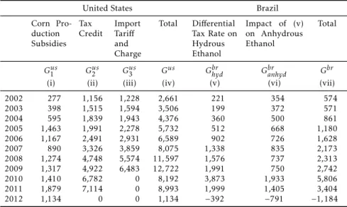
U.S. and Brazilian ethanol subsidy equivalent values in the 2002-12 period are presented in Table 3. Columns (i), (ii) and (iii) list the subsidy equivalent de-rived from corn production subsidies, tax credit and ethanol import barriers in the United States, which are calculated by equations 1, 2 and 3, respectively. The total subsidy equivalent for the ethanol production chain in the United States is summarized in column (iv). Columns (v) and (vi) list the subsidy equivalent derived from the Brazilian differential tax rate for hydrous ethanol
and gasoline and its indirect impact on the anhydrous ethanol market, which are given by equations 5 and 6, respectively. The total subsidy equivalent in Brazil is listed in column (vii). For each of the eleven years under analysis, the subsidy equivalent to ethanol production in the United States was signif-icantly higher than in Brazil. On average, the subsidy equivalent in Brazil corresponded to less than a quarter of the value in the United States.
Owing to the significant decline observed in U.S. and Brazilian policies for ethanol in 2012, we first describe and analyze the period 2002-11 and then the year 2012.
The subsidy equivalent value of ethanol-related policies in the United States increased from US$2.6 billion in 2002 to US$12.7 billion in 2009. About 46% of this support came from the import tariffand 40% from the tax credit
in 2002-2009. Tax credits became the dominant source of subsidies in 2010 and 2011, as the United States became a net exporter of ethanol and no market price support was recorded. Finally prorated feedstock subsidies accounted for the entirety of the total subsidy equivalent after ethanol tax credits were
7In the United States, economic incentives may cause ethanol demand to exceed the
su
re
m
en
t
of
et
h
an
ol
su
bs
id
ie
s
an
d
as
so
ci
at
ed
ec
on
om
ic
d
is
to
rt
io
n
s
46
7
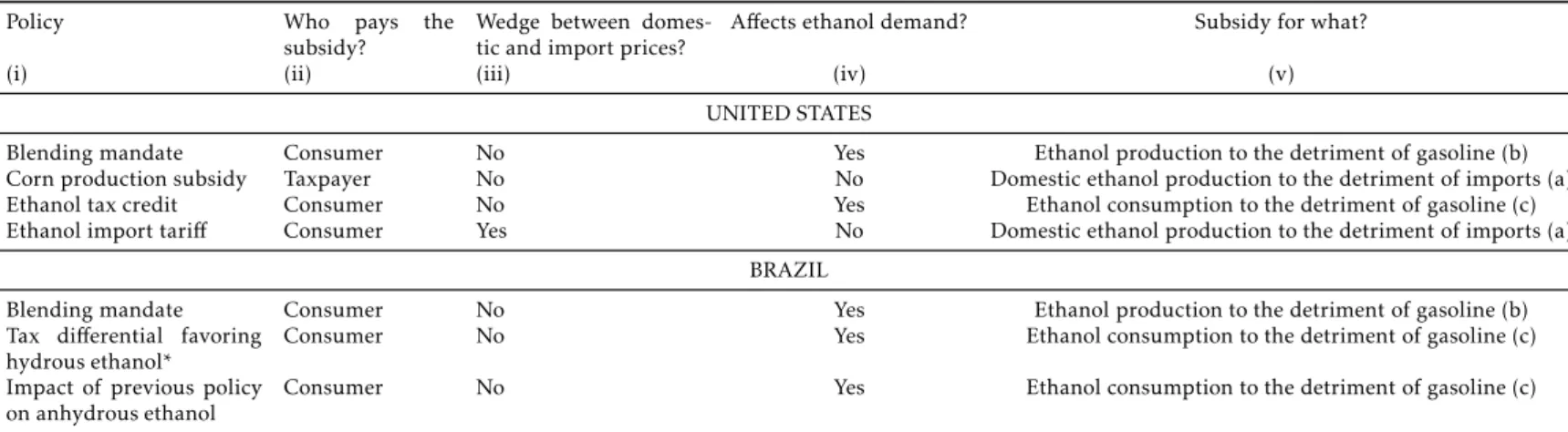
Table 2: Qualitative evaluation of U.S. and Brazilian ethanol policies
Policy Who pays the
subsidy? Wedge between domes-tic and import prices? A
ffects ethanol demand? Subsidy for what?
(i) (ii) (iii) (iv) (v)
UNITED STATES
Blending mandate Consumer No Yes Ethanol production to the detriment of gasoline (b) Corn production subsidy Taxpayer No No Domestic ethanol production to the detriment of imports (a) Ethanol tax credit Consumer No Yes Ethanol consumption to the detriment of gasoline (c) Ethanol import tariff Consumer Yes No Domestic ethanol production to the detriment of imports (a)
BRAZIL
Blending mandate Consumer No Yes Ethanol production to the detriment of gasoline (b) Tax differential favoring
hydrous ethanol* Consumer No Yes Ethanol consumption to the detriment of gasoline (c) Impact of previous policy
on anhydrous ethanol Consumer No Yes Ethanol consumption to the detriment of gasoline (c) Note: * Includes the tax equivalent rate of the difference between international and government-controlled domestic gasoline prices.
Table 3: Subsidy equivalent value, U.S. and Brazilian ethanol sectors, 2002-12 (million US$)
United States Brazil
Corn Pro-duction Subsidies
Tax
Credit ImportTariff and Charge
Total Differential Tax Rate on Hydrous Ethanol
Impact of (v) on Anhydrous Ethanol
Total
Gus1 Gus2 Gus3 Gus Ghydbr Gbranhyd Gbr
(i) (ii) (iii) (iv) (v) (vi) (vii)
2002 277 1,156 1,228 2,661 221 354 574
2003 398 1,515 1,594 3,506 199 372 571
2004 595 1,839 1,943 4,376 360 500 861
2005 1,463 1,991 2,278 5,732 512 668 1,180
2006 1,167 2,491 2,931 6,589 902 726 1,628
2007 890 3,326 3,859 8,075 1,338 835 2,173
2008 1,274 4,748 5,574 11,597 1,576 737 2,313 2009 1,317 4,922 6,483 12,722 1,991 750 2,742
2010 1,410 6,782 0 8,192 3,873 1,933 5,806
2011 1,879 7,114 0 8,993 1,999 1,405 3,404
2012 1,134 0 0 1,134 −392 −791 −1,184
Notes: The following exchange rates were used to convert Brazilian real into U.S. dollar (in R$ per US$): 2002 – 2.92; 2003 – 3.08; 2004 – 2.93; 2005 – 2.44; 2006 – 2.18; 2007 – 1.95; 2008 – 1.83; 2009 – 1.99; 2010 – 1.76; 2011 – 1.67 and 2012 – 1.95.
Source: Authors.
removed in 2012. Subsidies on the corn used by the ethanol industry were on average US$1 billion in 2002-12. Although the volume of corn used in ethanol production increased significantly over the last decade, total domes-tic support to corn fell considerably after 2005. As a result, domesdomes-tic support to corn used in ethanol production remained below the 2005 level in all years except 2011. Figure 8 depicts this behavior.
U.S ethanol subsidy estimates by Koplow (2007) corroborate the values described in this study. According to this author, total subsidies to the U.S. ethanol sector reached US$5.8-7 billion in 2006, US$6.9-8.4 billion in 2007, US$9.2-11 billion in 2008 and US$11-13.4 billion in 2009. The corresponding values found in the present study were US$6.5 billion in 2006, US$8.0 billion in 2007, US$11.5 billion in 2008 and US$12.7 billion in 2009.
Brazil’s ethanol subsidy equivalent increased signifincalty over the 2002-11 period. While total subsidies were in the order of US$574 million in 2002, they reached US$5.8 billion in 2010 and US$3.4 billion in 2011. National fig-ures correspond to the sum of subsidy equivalents for each of the 26 Brazilian states and the federal district, which vary significantly due to differences in
tax rates and consumption levels. The state of São Paulo alone accounted on average for 56% of Brazil’s ethanol subsidy equivalent in 2002-12.
The CIDE tax differential accounted for approximately 95% of the total
subsidy equivalent to the Brazilian ethanol sector in 2002-03. After a num-ber of states lowered their ICMS rates for ethanol, the share of the CIDE tax differential in the total subsidy equivalent fell to 68% in 2004-07. This share
dropped even further after the reduction of the CIDE rate in 2008. The ICMS tax differential exerted its greatest influence in 2011, accounting for 50% of
Source: Fapri (2013), USDA (2013a) and WTO (2013).
Figure 8: Volume of corn used in ethanol production and domestic
sup-port to corn and to corn used in ethanol production, United States, 2002-12
Another way to compare ethanol support is to consider their values rel-ative to the value of production in each country. This approach provides a more realistic picture of the level of subsidization, especially when the coun-tries under comparison have substantially different production volumes. In
the case of Brazil and the United States, ethanol production volumes were similar between 2003 and 2005, but increasingly disparate after 2006. No-tably, U.S. ethanol output was between 2 and 2.5 times higher than Brazil’s between 2007 and 2012.
Figure 9 presents ethanol subsidy equivalents relative to the total value of ethanol production in the United States and Brazil. Despite the increase in overall U.S. subsidy levels between 2002 and 2011, total subsidy equivalent as a share of the production value decreased from 65% in 2002 to 17% in 2011. In Brazil, the subsidy equivalent corresponded to 14% of the value of production on average between 2002 and 2011.
In stark contrast with earlier years, and reflecting the changes in policy described in Section 2, ethanol subsidy equivalent values declined in both countries in 2012. While subsidies as a percentage of the production value dropped by 83% in the United States, they became negative in Brazil (Figure 9 and Table 3). The reversal in subsidization in Brazil was due to gasoline price controls and the elimination of the CIDE (despite the continuation of the ICMS tax differential in some states). As opposed to 2010, the government
kept domestic gasoline prices below international prices in 2012. As a result, the subsidy equivalent value of Brazilian ethanol policies was US$−1.18
bil-lion in 2012, which correspond to −5% of the domestic ethanol production
Source: Authors.
Figure 9: Share of ethanol subsidy equivalents in domestic production
values, United States and Brazil, 2002-12
4
Impacts of ethanol subsidy equivalents
The objective of this section is to estimate the size of the market distortions caused by ethanol policies adopted in the United States and Brazil in each year of the period of 2002-12. The economic model used to estimate impacts on ethanol prices, production and consumption are described in Subsection 4.1. Results are discussed in Subsection 4.2.
4.1 Modeling framework
The model divides the world ethanol market into two segments: the United States and Brazil. As far as U.S. policies are concerned, this study considers only the support derived from import tariffs and the tax credit. Since the part
of the subsidy equivalent value arising from the domestic support to corn production is small, it is not taken into account here. In the case of Brazil, the markets for anhydrous and hydrous ethanol are analyzed jointly.8
The modeling of the world ethanol market is based on supply and demand functions in the United States and Brazil, as these two countries were responsi-ble for the bulk of global production and consumption in 2002-12. The model is described in equations 7 through 10:
8Given that most producers can switch production between hydrous and anhydrous ethanol
dlnSus=ǫus(1−α)dlnPw+αdlng3us
(7)
dlnSbr=ǫbrdlnPw (8)
dlnDus=ηus(1−β2−β3)dlnPw+β2dlng2us+β3dlng3us
(9)
dlnDbr=γηbr+ (1−γ)ηc,gbrθ
dlnPw+γηbrc + (1−γ)ηgbrθ
dlnPgbr (10)
whereSi,ǫi,Di andηi stand for supply, supply price elasticity, demand and
demand price elasticity in country i = us, br. Pw is the world ethanol price; α is the ratio of U.S. import tariffs to U.S. producer gross receipts, and β2
andβ3 are the ratios of, respectively, U.S. tax credits and U.S. import tariffs
to U.S. consumer final expenditures. In Section 3, subsidy equivalent val-ues for the United States (Gus2 and Gus3 ) were presented in monetary value. In the model presented in equations 9 through 10, g2us , g3us represent sub-sidy equivalent unit values. The Brazilian demand function is the weighted sum of demand functions for hydrous and anhydrous ethanol. While hydrous ethanol demand is multiplied by the share of hydrous ethanol in total ethanol fuel demanded (γ), anhydrous ethanol demand corresponds to the demand
for gasoline multiplied by the share of anhydrous ethanol in gasoline (θ) and
the share of anhydrous ethanol in total ethanol fuel demanded (1−γ). Pgbr is
the gasoline price in Brazil,ηgbr is the Brazilian price elasticity of demand for gasoline, ηc,gbr is the Brazilian cross-price demand elasticity for gasoline with
respect to ethanol, andηcbr is the Brazilian cross-price demand elasticity for
ethanol with respect to gasoline.
As explained in Section 2 and shown in Brazilian demand function, de-mand for ethanol in Brazil is also dependent on the price of gasoline. More-over, the subsidy equivalents that were previously described in terms of ethanol production, depending on how they are disposed of, initially affect the price
of gasoline in the country and then, indirectly, the price of ethanol. For ex-ample, if the differential tax between these fuels were removed, this could
either increase the tax on ethanol or reduce the tax on gasoline, whereas, if gasoline price controls were eliminated, there would be only a direct effect on
the price of fossil fuels. Therefore, market impacts from the elimination of ethanol support in Brazil (Gbr) are measured by considering direct impacts
on the gasoline price (dlnPgbr), as shown in equation 10.
World supply (Sw) is the sum of U.S. and Brazilian supplies:
dlnSw=δus
ǫus(1−α)dlnPw+αdlng3us
+δbrǫbrdlnPw (11)
whereδus and δbr are the shares of the United States and Brazil in world
ethanol production, respectively.
Similarly, world demand (Dw) is described in equation 12 as the sum of
U.S. and Brazilian demands:
dlnDw=φusηus
(1−β2−β3)dlnPw+β2dlng2us+β3dlng3us
+
+φbr
γηbr+ (1−γ)ηc,gbrθ
dlnPw+
γηbrc + (1−γ)ηbrg θ
dlnPgbr
whereφus and φbr are the shares of the United States and Brazil in world ethanol demand, respectively.
Letting world supply equal world demand and singling outdlnPw:
dlnPw=φ usηusβ
2 A dlng
us 2 +
h φ Adlng
us 3 +
+φ
br
γηcbr+ (1−γ)−µbrg θ
A dlnP
br g
(13)
whereA=
δusǫusα+δbrǫbr−φusηusα−φbr(γηbr+ (1−λ)ηc,gbrθ)
.
The magnitude of the impacts estimated in this study depends on the val-ues of the parameters described in equation 13. U.S. and Brazilian shares in world ethanol production and consumption were obtained from LMC (2008) and LMC (2013). Supply and demand elasticities for the United St tes were calculated as the simple averages of the elasticities estimated by Elobeid & Tokgoz (2008) and Luchansky & Monks (2009). While the former tudy uses U.S. supply and demand elasticities of respectively 0.65 and−0.43 the latter
estimates elasticities of 0.224 and−2.915. Therefore, the U.S. pri e elasticities
of supply and demand used in this study were 0.437 and −1.6725,
respec-tively.
The Brazilian supply elasticity of 1.94 was obtained in Costa et al. (2013a). Given that the change in the profile of Brazil’s automobile fleet in 2002-12 radically changed the behavior of consumers, the Brazilian price-elasticity of demand is assumed to vary throughout the period. While a demand elasticity of −1.23 (Farina et al. 2010) is used for 2002, an elasticity of−3.25 is used
for 2012 (Costa et al. 2013b). For 2003-11, a linear trend is assumed between the demand elasticities for 2002 and 2012. Demand cross-price elasticities for ethanol also vary between 1.45 in 2002 (Farina et al. 2010) and 2.68 in 2012 (Costa et al. 2013a). Demand price and cross-price elasticities for gasoline in
Brazil of−1.08 and 0.44 are obtained from Costa et al. (2013a).
Five alternative scenarios are considered in this study. Each scenario pre-supposes the elimination of a different set of ethanol support policies: U.S.
and Brazilian policies (Scenario 1), U.S. policies (Scenario 2), U.S. import tar-iffs alone (Scenario 3), U.S. tax credits alone (Scenario 4) and the Brazilian
policies (Scenario 5).
4.2 Results
Estimated market impacts due to the elimination of U.S. and Brazilian ethanol support are summarized in Table 4 (relative effects) and Table 5 (absolute
effects). Results for the 2002-11 period are analyzed separately from results
for 2012, as key ethanol support policies were discontinued in January 2012 in the United States and June 2012 in Brazil.
M ea su re m en t of et h an ol su bs id ie s an d as so ci at ed ec on om ic d is to rt io n s 47 3 support, 2002-12
2002 2003 2004 2005 2006 2007 2008 2009 2010 2011 2012
Relative Impact on Fuel Ethanol Prices
United States*
Scenario 1 −1.1% 1.2% 0.4% −1.2% −2.2% −2.5% −1.5% −3.3% 1.9% 5.0% 2.5%
Scenario 2 1.7% 3.7% 3.5% 1.6% 0.8% 1.4% 1.5% 0.5% 7.9% 6.9% 0.0%
Scenario 3 −15.2% −13.7% −13.1% −10.6% −8.5% −9.3% −7.9% −8.9% 0.0% 0.0% 0.0% Scenario 4 16.8% 17.2% 16.5% 12.1% 9.3% 10.6% 9.4% 9.3% 7.9% 6.9% 0.0% Scenario 5 −2.2% −1.8% −2.3% −2.2% −2.5% −3.2% −2.4% −3.1% −5.7% −1.8% 2.5%
Brazil
Scenario 1 0.6% 2.9% 2.1% 1.9% 0.8% 0.5% 1.5% 2.0% −12.9% −8.2% 2.5% Scenario 2 3.5% 5.4% 5.2% 4.8% 3.8% 4.5% 4.5% 5.8% −6.9% −6.4% 0.0% Scenario 3 14.7% 19.8% 18.7% 14.6% 11.5% 12.9% 12.4% 13.1% 0.0% 0.0% 0.0% Scenario 4 −11.3% −14.6% −13.6% −9.9% −7.7% −8.5% −7.9% −7.3% −6.9% −6.4% 0.0% Scenario 5 −2.2% −1.8% −2.3% −2.2% −2.5% −3.2% −2.4% −3.1% −5.7% −1.8% 2.5%
Relative Impact on Fuel Ethanol Production
United States*
Scenario 1 −12.9% −13.8% −13.3% −10.4% −8.5% −9.5% −8.3% −8.9% −5.7% −3.6% 1.1% Scenario 2 −12.0% −13.1% −12.3% −9.4% −7.4% −8.2% −7.3% −7.6% −3.0% −2.8% 0.0% Scenario 3 −8.6% −8.9% −8.3% −6.2% −4.7% −5.3% −4.6% −5.1% 0.0% 0.0% 0.0% Scenario 4 −5.0% −6.4% −6.0% −4.3% −3.4% −3.7% −3.5% −3.2% −3.0% −2.8% 0.0% Scenario 5 −1.0% −0.8% −1.0% −1.0% −1.1% −1.4% −1.1% −1.3% −2.5% −0.8% 1.1%
Brazil
Scenario 1 1.2% 5.6% 4.0% 3.8% 1.5% 1.1% 2.9% 3.9% −25.1% −16.0% 4.9% Scenario 2 6.7% 10.4% 10.1% 9.3% 7.4% 8.6% 8.7% 11.2% −13.3% −12.4% 0.0% Scenario 3 28.6% 38.4% 36.3% 28.4% 22.3% 25.1% 24.0% 25.4% 0.0% 0.0% 0.0% Scenario 4 −22.0% −28.3% −26.4% −19.3% −15.0% −16.6% −15.4% −14.2% −13.3% −12.4% 0.0% Scenario 5 −4.2% −3.4% −4.4% −4.3% −4.9% −6.1% −4.7% −6.0% −11.0% −3.4% 4.9%
Relative Impact on Fuel Ethanol Consumption
United States*
Scenario 1 2.8% 1.2% 1.6% 3.8% 4.4% 4.5% 3.2% 6.2% −6.5% −12.3% −4.4% Scenario 2 0.6% −0.4% −0.5% 1.1% 1.0% 0.8% 0.3% 2.7% −15.5% −15.6% 0.0% Scenario 3 36.1% 37.8% 32.8% 25.3% 19.0% 19.9% 16.0% 18.0% 0.0% 0.0% 0.0% Scenario 4 −36.9% −40.7% −35.4% −25.4% −18.6% −20.1% −16.5% −16.2% −15.5% −15.6% 0.0% Scenario 5 4.0% 3.3% 3.9% 3.9% 4.4% 5.2% 3.7% 4.7% 9.8% 3.5% −4.4%
Brazil
Scenario 1 −13.2% −12.0% −14.2% −15.9% −20.5% −22.0% −18.5% −24.5% −24.0% −2.5% 21.2% Scenario 2 −1.8% −2.9% −3.5% −3.9% −4.4% −5.8% −6.7% −10.0% 13.5% 12.9% 0.0% Scenario 3 −7.6% −10.9% −12.6% −12.0% −13.3% −17.0% −18.4% −22.5% 0.0% 0.0% 0.0% Scenario 4 5.8% 8.0% 9.2% 8.1% 9.0% 11.2% 11.8% 12.6% 13.5% 12.9% 0.0% Scenario 5 −11.7% −9.5% −11.3% −12.5% −16.7% −17.2% −12.6% −15.8% −38.3% −15.7% 21.2% Notes: * Domestic support for corn production not considered.
Scenario 1: Elimination of U.S. and Brazilian ethanol support. Scenario 2: Elimination of U.S. ethanol support.
Ja
le
s
e
C
os
ta
E
co
n
om
ia
A
p
lic
ad
a,
v.1
8
,
n
.3
ethanol support, 2002-12
2002 2003 2004 2005 2006 2007 2008 2009 2010 2011 2012
Absolute Impact on Fuel Ethanol Production (million liters)
United States*
Scenario 1 −1,044 −1,464 −1,712 −1,534 −1,566 −2,353 −2,941 −3,691 −2,849 −1,904 552 Scenario 2 −973 −1,387 −1,591 −1,397 −1,369 −2,025 −2,576 −3,156 −1,512 −1,471 0 Scenario 3 −693 −941 −1,073 −920 −872 −1,314 −1,610 −2,127 0 0 0 Scenario 4 −401 −678 −767 −642 −624 −921 −1,219 −1,329 −1,512 −1,471 0 Scenario 5 −78 −82 −128 −143 −204 −340 −374 −558 −1,251 −406 552
Brazil
Scenario 1 154 591 461 475 218 163 467 690 −5,647 −4,403 1,019 Scenario 2 873 1,102 1,166 1,169 1,096 1,332 1,387 1,993 −2,997 −3,403 0 Scenario 3 3,722 4,072 4,183 3,585 3,305 3,869 3,820 4,505 0 0 0 Scenario 4 −2,864 −3,002 −3,047 −2,433 −2,219 −2,552 −2,447 −2,531 −2,997 −3,403 0 Scenario 5 −553 −361 −509 −543 −724 −943 −751 −1,063 −2,479 −940 1,019
Absolute Impact on Fuel Ethanol Consumption (million liters)
United States*
Scenario 1 283 132 213 587 913 1,161 1,148 2,594 −3,170 −5,818 −2,202
Scenario 2 57 −40 −65 177 216 195 117 1,110 −7,495 −7,368 0
Scenario 3 3,703 4,040 4,406 3,906 3,908 5,135 5,808 7,517 0 0 0 Scenario 4 −3,784 −4,350 −4,758 −3,917 −3,833 −5,173 −5,970 −6,747 −7,495 −7,368 0 Scenario 5 414 350 526 608 913 1,330 1,350 1,974 4,751 1,680 −2,202
Brazil
Scenario 1 −1,173 −1,006 −1,464 −1,646 −2,262 −3,352 −3,622 −5,595 −5,325 −489 3,774 Scenario 2 −158 −246 −361 −405 −489 −888 −1,306 −2,273 2,985 2,493 0 Scenario 3 −674 −909 −1,295 −1,240 −1,475 −2,579 −3,597 −5,139 0 0 0
Scenario 4 519 670 944 842 990 1,701 2,304 2,887 2,985 2,493 0
Scenario 5 −1,045 −793 −1,164 −1,294 −1,841 −2,614 −2,475 −3,595 −8,480 −3,027 3,774 Notes: * Domestic support for corn production not considered.
Scenario 1: Elimination of U.S. and Brazilian ethanol support. Scenario 2: Elimination of U.S. ethanol support.
The elimination of U.S. support alone (Scenario 2) increases U.S. and Brazil-ian ethanol prices on average by 2.4% and 3%, respectively, in 2002-11. Pro-duction decreases by 8.3% in the United States, but increases by 4.7% in Brazil.9 Consumption levels fall by 2.5% in the former and 1.3% in the
lat-ter. However, 2002-11 averages for Brazil hide significant intra-period vari-ation: while production expands on average by 9.1% in 2002-09, it falls by 12.9% in 2010-11. Similarly, Brazilian consumption declines on average by 4.9% in 2002-09 and rises by 13.2% in 2010-11. Brazilian output increases and consumption falls in 2002-09 because the effects from eliminating U.S.
import tariffs overshadow those from removing U.S. tax credits. The situation
is reversed in 2010-11, as U.S. market price support is null in this sub-period. The removal of U.S. import tariffs alone (Scenario 3) reduces U.S. ethanol
prices on average by 8.7% in 2002-11, which leads to an average increase of 20.5% in U.S. consumption. The elimination of U.S. tax credits alone (Scenario 4) generates diametrically opposite results: U.S. ethanol prices increase on average by 11.6% and domestic consumption decreases by 24.1% in the same period. U.S. production decreases in both scenarios (5.2% in Scenario 3 and 4.1% in Scenario). In Brazil, prices rise by 11.8%, consumption decreases on average by 11.4% and production increases by 22.8% in Scenario 3. Results for the Brazilian ethanol market in Scenario 4 are the inverse: prices fall by 9.4%, consumption increases by 10.2% and production decreases by 18.3%.
The greatest absolute changes in production and consumption volumes in Scenario 3 occur in 2009, when Brazilian ethanol production increase by 4.5 billion liters and U.S. consumption increases by 7.5 billion liters. In Scenario 4, the greatest absolute changes occur between 2009 and 2011: Brazilian pro-duction decreases by 3.4 billion liters in 2010 and U.S. consumption falls by 7.5 billion liters in 2009.
The elimination of Brazil’s ethanol support alone (Scenario 5) leads to an average reduction of 2.7% in ethanol prices in both countries in 2002-11. Pro-duction volumes in the United States and Brazil fall on average by 1.2% and 5.3% in the same period. While U.S. consumption increases by 4.7%, Brazilian consumption declines by 16.1%, as the average reduction in domestic gasoline prices (19.3%) is considerably greater than the decline in ethanol prices. The most pronounced market changes in Scenario 5 occur in 2010, the year with the greatest mark-up in Brazilian gasoline prices relative to the international market: Brazilian ethanol price, production and consumption levels undergo retractions of respectively 5.7%, 11.0% and 38.3%, which are more than twice as great as the average reductions for the 2002-11 period as whole.
As the domestic gasoline price in Brazil was kept below the world price in 2012, the direction of market changes implied by Scenario 5 in this particu-lar year is the opposite of that for 2002-11: Brazilian ethanol price, produc-tion and consumpproduc-tion levels increase by 2.5%, 4.9% and 21.2%, respectively. While U.S. policies depressed world ethanol prices in 2002-11, Brazilian poli-cies were responsible for constraining prices in 2012. As a result, Brazil’s gaso-line price controls adversely affected ethanol production domestically and in
the United States in 2012.
Considering the results reported above for the five alternative policy re-form scenarios, most distortions in ethanol markets in 2002-11 can be traced
9Output expansion is dependent on area availability. This potential limitation is not
back to measures applied by the United States. While U.S. policies decreased world prices and adversely affected Brazilian production in 2002-09 (Scenario
2), Brazilian policies led to higher international prices and boosted production in both countries in 2002-11 (Scenario 5). Artificially low Brazilian gasoline prices in 2012 negatively affected ethanol prices and production both
domesti-cally and in the United States. Nonetheless, the deleterious effects of Brazilian
gasoline price controls on ethanol output in 2012 were greater domestically (4.9% retraction) than in the United States (1.1% reduction).
Among the five scenarios analyzed above, the elimination of U.S. ethanol import tariffs (Scenario 3) has by far the greatest impact on world prices
(aver-age increase of 11.8% in 2002-11). In addition, the elimination of U.S. ethanol tariffs could generate positive environmental effects. While corn ethanol
pro-duction would on average decrease by 5.2% in 2002-11, sugarcane ethanol output would increase by 22.8% in the same period. Lifecycle analyses indi-cate that ethanol derived from sugarcane reduces greenhouse gas emissions by 90% relative to conventional gasoline, while the reduction for ethanol de-rived from corn is of only 10-30% (IEA 2009). Moreover, Brazilian sugar-cane ethanol is more productive than U.S. corn ethanol in terms of liters per hectare planted. While one hectare of sugarcane in Brazil yields 6,800 liters of ethanol, one hectare of corn in the United States yields only 3,100 liters. Fur-thermore, the energy balance of Brazilian sugarcane ethanol is five times as high as that of U.S. corn ethanol (Worldwatch Institute 2006). Consequently, the elimination of U.S. import tariffs and additional charges would generate
environmental benefits due to the replacement of corn ethanol by sugarcane ethanol.
Given the elimination of significant U.S. and Brazilian ethanol policies in 2012, it is possible to test the model used in this study by comparing estimated market changes with actual observed variations between 2011 and 2012. Esti-mated and observed ethanol price, production and consumption changes are depicted in Figure 10. Estimated changes correspond to the results from the elimination of U.S. and Brazilian policies (Scenario 1) in 2011 inus the shock from eliminating the policies that remained in place in 2012.
While estimated price, production and consumption relative changes in the United States were respectively 2.0%, −3.5% and−4.3%, those actually
observed were −2.5%,−3.3%, and 3.5%. In Brazil, estimated changes were −11.2% for the domestic price,−6.4% for production and−5.6% for
consump-tion. Those observed were−2.6%,−5.1% and−2.1%. Although estimated
pro-duction changes followed observed changes closely, estimated and observed price and consumption changes were not as close. The differences between
observed and estimated price and consumption in Brazil can be explained by the domestic sugarcane crop failure. Two factors may have contributed to the difference between estimated and observed price changes in the United States:
Source: Authors.
Figure 10: Observed and estimated percent changes in ethanol prices, pro-duction and consumption in the United States and Brazil, from 2011 to 2012
Small differences between estimated and observed market changes in 2012
may also be explained by limitations in the model. First, the elasticity values adopted may not exactly express the market behavior when policies changed. Second, elasticities are generally appropriate for small changes, but are not very well defined for the large changes that occurred in 2012. Finally, subsi-dies are not the only forces that influence producer and consumer behavior. Crop failures, economic growth and technology changes are some of these other factors. Figure 11 illustrates the results of a sensitivity analysis with four different sets of supply and demand price elasticities: (i) all elasticities
are 10% higher; (ii) all elasticities are 10% lower; (iii) Brazilian elasticities are 10% higher and U.S. elasticities are 10% lower; and (iv) Brazilian elasticities are 10% lower and U.S. elasticities are 10% higher. The sensitivity analysis was applied only to Scenario 1 and Scenario 5, as production and consump-tion effects in the other scenarios were null in 2012.
As indicated in Figure 11, estimated results vary little when elasticities are increased or decreased by 10%. This sensitive analysis suggests that elasticity values are not the main source of variation between estimated and observed changes identified in Figure 10.
5
Conclusion
Source: Authors.
Figure 11: Estimated relative changes in production and consumption under alternative sets of elasticities, Scenarios 1 and 5, 2012
magnitude of biofuel subsidies and their market impacts. The present study contributes to this discussion by providing estimates of the subsidy equivalent values of ethanol policies in the United States and Brazil, the world’s leading biofuel producers. For 2002-11, average annual ethanol subsidy levels were US$7.2 billion in the United States and US$2.1 billion in Brazil. These fig-ures were equivalent to approximately 48% of the value of domestic ethanol production in the United States and 14% in Brazil.
The study also estimates the effects of U.S. and Brazilian ethanol
subsi-dies on prices, production and consumption. While U.S. ethanol policies pro-vided incentives to domestic production at the expense of imports in 2002-11, Brazilian policies encouraged production without discriminating between do-mestic and foreign ethanol. As a result, foreign producers were adversely affected by the former, but benefited from the latter. U.S. ethanol policies
de-pressed world prices by 2.4% on average in 2002-11, whereas Brazilian poli-cies boosted prices by 2.7% in the same period. The negative market effects
pos-sible reactivation of ethanol tax credits and import tariffs. Given that the
ethanol blending mandate in the United States will increase from 15.2 billion gallons in 2012 to 36 billion gallons in 2022, market distortions caused by U.S. policies could significantly increase in the near future if import barriers and tax credits were reinstated. Distortions would be even larger if import tariffs
were reintroduced alone.
The period examined in this study covers significant policy changes not only in the United States, but also in Brazil. Most notably, U.S. ethanol import tariffs and tax credits were eliminated in January 2012 and Brazil’s CIDE tax
differential was removed in June 2012. In addition, Brazilian gasoline price
controls, which kept domestic prices above world prices in 2002-11, were re-versed in 2012, causing Brazilian gasoline prices to be below international prices for the first time in a decade. While U.S. policies reduced ethanol pro-duction in Brazil prior to 2011, Brazilian gasoline price controls were responsi-ble for reducing domestic ethanol output by 5% in 2012. Therefore, domestic policies became the main source of adverse effects on Brazil’s ethanol market.
Biofuels provide a great possibility for the substitution of carbon-intensive fossil fuels. Brazil and the United States have championed a transformation in transportation fuel use with public policies that encourage the adoption of ethanol. However, these same policies generate distortions that may jeop-ardize the consolidation of an international market for ethanol. The subsidy equivalent values and market distortion estimates presented in this study pro-vide U.S and Brazilian policymakers with vital inputs for the assessment of the multifaceted implications of ethanol support.
Acknowledgments
The authors thanks the National Center of Scientific and Technological Devel-opment (CNPq).
Bibliography
ANP (2013a), ‘Dados estatísticos mensais: vendas de combustíveis’.
URL:Avaiable at http://www.anp.gov.br/petro/dados_estatisticos.asp/, Accessed in 2013-09-17
ANP (2013b), ‘Levantamento de preços e de margem de comercialização de combustíveis, coordenadoria de defesa da concorrência’.
URL:Avaiable at http://www.anp.gov.br/petro/relatorios_precos.asp/, Accessed in 2013-09-02
Brazilian Ministry of Finance (2013), ‘DCide (lei no. 10.336, de 19/12/2001)’.
URL:Avaiable at http://www.receita.fazenda.gov.br/PessoaJuridica/CIDEComb/, Accessed in 2013-09-17
Costa, C. C., Burnquist, H. L., Souza, M. J. P., Rodrigues, L. & Constanza, V. (2013b), Fuel demand in Brazil and consumer choice between ethanol and gasoline. Research report. Unpublished.
Costa, C. C. & Guilhoto, J. J. M. (2011), ‘O papel da tributação diferenciada dos combustíveis no desenvolvimento econômico do estado de São Paulo’,
Economia Aplicada15(3), 371–392.
Elobeid, A. & Tokgoz, S. (2008), ‘Removing distortions in the U.S. ethanol market: What does it imply for the United States and Brazil?’,American Jour-nal of Agricultural Economics90(4), 918–932.
FAO (2013), ‘United Nations Commodity Trade Statistics database — COM-TRADE’.
URL:Avaiable at http://comtrade.un.org/db/, Accessed in 2013-02-02
Fapri (2013), ‘U.S. and world agricultural outlook database’.
URL: Avaiable at http://www.fapri.iastate.edu/tools/outlook.aspx, Accessed in 2013-05-14
Farina, E., Viegas, C., Pereda, P. & Garcia, C. (2010), Estruturas de mercado e concorrência do setor de etanol,inE. L. Sousa & I. C. Macedo, eds, ‘Etanol e
bioeletricidade: a cana-de-açúcar no futuro da matriz energética’, São Paulo: Luc Projetos de Comunicação, pp. 226–259.
IEA (2009), ‘CO2 Emissions from Fuel Combustion: Highlights’.
URL:Avaiable at http://www.iea.org/co2highlights/CO2highlights.pdf, Accessed in 2010-04-20
Koplow, D. (2007), ‘Biofuels — at what cost? government support for ethanol and biodiesel in the United States: 2007 update’.
URL: Avaiable at http://www.globalsubsidies.org/files/assets/Brochure_-_US_Update.pdf, Accessed in 2009-12-10
LMC (2008), Ethanol Quarterly - 4th Quarter, 2008, Technical report, Ox-ford: LMC International.
LMC (2013), Ethanol Quarterly - 1st Quarter, 2013, Technical report, Oxford: LMC International.
Luchansky, M. S. & Monks, J. (2009), ‘Supply and demand elasticities in the US ethanol fuel market’,Energy Economics31(3), 403–410.
MDIC (2013), ‘Ministério do Desenvolvimento, Indústria e Comércio Exte-rior. Comércio ExteExte-rior. Estatísticas de Comércio ExteExte-rior. Aliceweb’.
URL:Avaiable at http://aliceweb.desenvolvimento.gov.br, Accessed in 2013-02-03
OECD (2008), ‘OECD’s Producer Support Estimate and Related Indicators of Agricultural Support: Concepts, Calculations, Interpretation and Use (The PSE Manual)’.
Tyner, W. E. (2008), ‘The US ethanol and biofuels boom: Its origins, current status, and future prospects’,BioScience58(7), 646–653.
UNICA (2013a), ‘Quotes&Stats’.
URL:Avaiable at http://www.unica.com.br, Accessed in 2013-09-10
UNICA (2013b), ‘Unicadata — Veículos automotores — Veículos — Frota’.
URL:Avaiable at http://www.unica.com.br, Accessed in 2013-03-03
USDA (2013a), ‘CCC budget essentials’.
URL: Avaiable at http://www.fsa.usda.gov/FSA/webapp?area=about&-subject=landing&topic=bap-bu-cc, Accessed in 2013-09-13
USDA (2013b), ‘World Agricultural Supply and Demand Estimates (WASDE), World Agricultural Outlook Board (WAOB)’.
URL:Avaiable at http://www.usda.gov/oce/commodity/wasde/, Accessed in 2013-10-12
USITC (2013), ‘Interactive Tariffand Trade DataWeb’.
URL:Avaiable at http://dataweb.usitc.gov/scripts/user_set.asp, Accessed in 2013-09-23
Worldwatch Institute (2006), Biofuels for Transportation: Global Potential and Implications for Sustainable Agriculture and Energy in the 21st Century, Washington,D.C.