Pesqui. Oper. vol.20 número1

(1)

MINIMIZING FLOWTIME SUBJECT TO OPTIMAL MAKESPAN ON TWO

IDENTICAL PARALLEL MACHINES

Jatinder N. D. Guptaa Johnny C. Hob

a

Department of Management, Ball State University, Muncie, IN 47306-0350, USA

b

Abbott Turner College of Business, Columbus State University, Columbus, GA 31907-5645, USA

Abstract

We consider the problem of scheduling jobs on two parallel identical machines where an optimal schedule is defined as one that gives the smallest total flowtime (the sum of the completion time of all jobs) among the set of schedules with optimal makespan (the completion time of the latest job). Utilizing an existing optimization algorithm for the minimization of makespan, we propose an algorithm to determine optimal schedules for this problem. We empirically show that the proposed algorithm can quickly find optimal schedules for problems containing a large number of jobs.

(2)

1. Introduction

Consider the following scheduling problem: a set

N

=

{

1 ,

2 ,

K

,

n

}

of

n

jobs available at time zero is to be processed on

m

identical parallel machines. Each job

i

∈

N

is to be processed without interruption on one of the

m

machines with processing time

p

_i. Each machine can process only one job at a time and no job may be processed by more than one machine. Setup time, if any, is included in the processing time. It is desired to minimize the makespan (maximum completion time) as the primary objective and minimize total flow-time (sum of the completion times of all jobs) as the secondary objective. Thus, it is required to find a schedule for which the total flowtime time is minimized, subject to the constraint that no reduction in the total makespan is possible. Both makespan and flowtime performance measures have significant impact on a schedule’s cost, since the former generally represents the amount of resources tied to a set of jobs; while the latter is a useful indicator of the amount of work-in-process. Parallel-machine scheduling problems often arise in practice as in the scheduling of jobs to a number of computer processors or the scheduling of jobs to a set of identical lathes.

The need to consider multiple criteria in scheduling is widely recognized. Either a simultaneous or a hierarchical approach can be adopted. For simultaneous optimization, there are two approaches. First, all efficient schedules can be generated, where an efficient schedule is one in which any improvement to the performance with respect to one of the criteria causes a deterioration with respect to one of the other criteria. Second, a single objective function can be constructed, for example by forming a linear combination of the various criteria, which is then optimized. Under a hierarchical approach, the criteria are ranked in order of importance; the first criterion is optimized first, the second criterion is then optimized, subject to achieving the optimum with respect to the first criterion, and so on. Surveys of algorithms and complexity results in this area are given by Chen and Bulfin (1993), Lee and Vairaktarakis (1993) and Nagar, Haddock, and Heragu (1995). Clearly, the above described problem is one of hierarchical multi-criteria scheduling.

Following the three field notation of scheduling problems, we will designate the identical parallel machine problem to minimize makespan subject to minimum total flowtime as a

)

(

||

F

∑

C

max

P

h i problem where

P

designates the identical parallel machines,

C

max denotes

the maximum completion time (makespan),

∑

C

i represents the total flowtime, and the functional notation

F

h

(

∑

C

i

C

max

)

designates that we hierarchically minimize total flowtime subject to minimum makespan.

The

P

||

∑

C

_i problem can be optimally solved using the extension of McNaughton’s algorithm (1959). As discussed by Conway et al (1967), this algorithm involves two steps: (1) order all

n

jobs in smallest processing time (SPT) order; and (2) assign the jobs from the SPT list to the

m

parallel machines in rotation. On the other hand, as shown by Bruno, Coffman, and Sethi (1974) and Garey and Johnson (1979),

P

||

C

_max problem is known to be NP-hard. In view of the above results, it follows that the

P

||

F

_h

(

∑

C

_i

C

_max

)

problem is also NP-hard.

(3)

3.7037% above the makespan of the optimal schedule. Eck and Pinedo's algorithm generates the schedule by arranging the differences according to LPT rule.

This paper proposes an optimization algorithm to minimize total flowtime among the set of makespan-optimal schedules for the two parallel machines problem, represented as a

)

(

||

2 F

∑

C

_max

P

h i problem. The rest of the paper is organized as follows: Section 2 introduces the assumptions and notation used to define and represent the

P

||

F

h

(

∑

C

i

C

_max

)

problem. Section 3 discusses the proposed optimization algorithm for the

P

2 ||

F

h

(

∑

C

i

C

_max

)

problem and provides numerical examples to demonstrate the proposed algorithm. The simulation experiment and computational results are given in Section 4. Finally, we conclude the paper in Section 5 with some fruitful directions for future research.

2. Problem Definition and Representation

The shop environment we consider consists of a set of

n

jobs to be processed by

m

parallel identical machines. Each job requires one operation, and each operation can be processed by either one of the available

m

machines. The objective is to minimize total flowtime subject to minimum total makespan.

Without loss of generality, we assume that the jobs are sorted according to the LPT order and that enough artificial jobs with zero processing time are added to the set of jobs if the total number of jobs

n

is not an integer multiple of the number of machines

m

. In other words, we assume that the total number of jobs

n

is an integer multiple of the number of machines

m

and that jobs are so numbered that

p

₁

≥

p

₂

≥

_K

,

≥

p

_n

.

The major assumptions used in this paper are listed below:

• Job’s processing time is known and deterministic.

• Job preemption is not allowed, i.e., once a job starts processing on a machine, it must finish processing on that machine without interruption.

• All jobs have the same ready time at zero.

• No precedence relationships among jobs.

• Each machine can process only one job at a time.

• Setup time is included in processing time.

We use the following notation in the problem formulation.

max

C

optimal makespan. i

p

processing time for job

i

.

ij

x

a binary variable which has a value of 1 if job

i

is assigned to machine

j

,

and 0 otherwise.

f

total flowtime. i

q

the weight assigned to job

i

when computing flowtime.

(4)

makespan,

C

max

,

while the second level of the model minimizes the flowtime subject to the optimal makespan found in the first level.

First Level Integer Program

Minimize

C

_max (1)

subject to:

∑

=

≥

−

n i ij i

x

p

C

1

max

0 ;

j

=

1 ,

2 ,

K

,

m

(2)

;

1

=

∑

= m j ij

x

i

=

1 ,

2 ,

K

,

n

(3)

;

1 or

0 =

ij

x

i

=

1 ,

2 ,

K

,

n

;

j

=

1 ,

2 ,

K

,

m

(4)

Second Level Integer Program

Minimize

∑ ∑

= =













=

m j n i i ij i

x

q

p

f

1 1 (5) subject to:

∑

=

≥

−

n i ij i

x

p

C

1

max

0 ;

j

=

1 ,

2 ,

K

,

m

(6)

;

1

=

∑

= m j ij

x

i

=

1 ,

2 ,

K

,

n

(7)

0

1

=









−

_∑

= ij i k kj i

x

q

i

=

1 ,

2 ,

_K

,

n

;

j

=

1 ,

2 ,

_K

,

m

(8)

;

1 or

0 =

ij

x

i

=

1 ,

2 ,

K

,

n

;

j

=

1 ,

2 ,

K

,

m

(9)

The above problem formulation in relations (1) through (9) is a bi-level non-linear integer program which is very difficult to solve. While it can be simplified for the two-machine case (by defining a binary variable

x

i

=

1

if job

i

is assigned to machine 1 and 0 otherwise); it still remains a bi-level non-linear integer program. Hence, we need to develop some alternative optimization methods for its solution. In this paper, we develop a lexicographic search based algorithm to solve

P

2 ||

F

_h

(

∑

C

_i

C

_max

)

problem.

3.The Proposed Optimization Algorithm

Ho and Wong (1995) developed a lexicographic search based algorithm for optimally solving the

max

||

2 C

P

problem. While the computational complexity of this algorithm is exponential, empirical results show that this algorithm is quite efficient in solving the

P

2 ||

C

max problem.

Therefore, we modify and extend this algorithm to develop an optimization algorithm for the

)

(

||

2 F

∑

C

_max

(5)

The development of the optimization algorithm is pursued in two parts. In the first part, we assume that we know the optimal makespan schedule

S

with makespan value

α

* where the jobs on each of the two machines are processed in an SPT order giving a total flowtime

β

. Our first algorithm, obtained by a modification of the TMO algorithm developed by Ho and Wong (1995) finds a schedule with a minimum possible total flowtime given that its makespan is

α

*. In the second part, we use the TMO algorithm to find a schedule with optimal makespan value and also find a schedule which has a minimum makespan given optimal total flowtime value.

3.1. Solving the

P

2 ||

F

h

(

∑

C

i

C

max

=

α

*

)

Problem

To describe an optimization algorithm for the

P

2 ||

F

_h

(

∑

C

_i

C

_max

=

α

*

)

problem, we define the following additional notations.

Sum

the sum of the processing time of all jobs. l

rest

the sum of the processing time of the set of jobs with indices

>

l

. i

N

the node at level

l

. i

V

the value of node

N

_i.

Z

the current incumbent total flowtime.

S

′′

the schedule defined as follows: the path from the root node to the node that generates

*

α

makespan represents the set of jobs assigned to machine 1, the rest of the jobs are assigned to machine 2 where jobs on each machine are in SPT order.

β ′′

the total flowtime of schedule

S

′′

For solving the

P

2 ||

F

_h

(

∑

C

_i

C

_max

=

α

*

)

problem, we use a binary tree to develop a lexicographic search based algorithm. The root node at level 0 has a value of 0. At each level,

,

2 ,

1 n

l

=

_K

in the tree, a given job is added to the partial schedule developed at the previous level. Any node at level

l

takes on one of two possible values as follows. If

N

_i is its parent’s left child, which means that job

l

is assigned to machine 1, then the value of

N

_i is its parent’s value plus the processing time of job

l

. If it is the right child, which indicates job

l

is assigned to machine 2, then the node has the same value as its parent’s. The makespan for machine 1 is denoted by the value of the leaf; while the makespan for the schedule equals to the larger of the makespan of machine 1 and the sum of the processing time of all jobs minus the makespan of machine 1. The paths from the root node to the nodes with makespan

α

* constitute the set of schedules that need to be evaluated. Following the above reasoning, the steps of the modified TMO algorithm are as follows:

Algorithm M: (Modified TMO Algorithm)

Input:

n

even,

p

i where

p

1

≥

p

2

≥

K

,

≥

p

n

,

schedule

S

with makespan

*

α

and total flowtime

β

where jobs on each machine in schedule

S

are processed in an SPT order. Step 1: Set

Z

=

β

and

S

′′

=

S

. Calculate

Sum

=

∑

ni₌1

p

i and

=

∑

=+

n l i i

l

p

rest

1

,

for

1 ,

,

2 ,

1 −

=

n

l

K

; and

rest

n

=

0

. If

* 1

=

α

(6)

otherwise mark the right child of the root node dead (because of the symmetry between the two machines).

Step 2: • If there is no living node, go to step 3. (Note that searching starts from the current node through a depth-first searching scheme.)

• Find the first living node through depth-first search, if it is at level

n

, then restart Step 2.

• Expand this node. If it doesn't have a left child, then its left child,

N

_i, is generated; otherwise, its right child,

N

_i, is generated.

• If

N

_i is its parent’s right child, then mark parent dead.

• If

max{

V

_i

,

(

Sum

−

V

_i

)}

=

α

* and

Z

<

β ′′

, set

Z

=

β ′′

and

S

*

=

S

′′

. If

max{

V

_i

,

(

Sum

−

V

_i

)}

=

α

*, restart Step 2.

• If

V

i

>

α

*, mark

N

i dead and restart Step 2.

• Let

l

be the level which

N

i is on.

• If

V

_i

+

rest

_l

<

Sum

−

α

*, mark

N

_i dead.

• Restart Step 2.

Step 3: Stop. The schedule

S

* yields the minimum total flowtime schedule

Z

given makespan =

.

*

α

The algorithm M described above is designed to determine all schedules with makespan =

α

*. Hence, it terminates only if

p

1

=

α

* (Step 1) or there is no living node (Step 2). Whenever a

makespan schedule with makespan =

α

* is found, algorithm M updates

Z

and

S

* if the total flowtime of the optimal makespan schedule is less than

Z

. To avoid the unnecessary search of nodes, the criteria used in the TMO algorithm to mark dead nodes are also applied in algorithm M.

3.2 Solving the

P

2 ||

F

_h

(

C

_max

∑

C

_i

)

Problem

In our solution to the

P

2 ||

F

h

(

∑

C

i

C

_max

)

problem, we will need to solve another hierarchical criteria problem of minimizing makespan subject to minimum total flowtime, the

)

(

||

2 F

h

C

max

∑

C

i

P

problem. From the analysis of the

P

2 ||

∑

C

_i problem by Conway, Maxwell, and Miller (1967), it follows that if jobs are arranged in the LPT (longest processing time) order, then, a pair of jobs at sequence positions

2 i

−

1

and

2 i

are processed on different machines. Therefore, arranging the jobs in the LPT order, Eck and Pinedo (1993) defined an alternative

P

2 ||

C

_max problem where the processing time of job

i

,

d

_i

=

p

₂_i₋₁

−

p

₂_i (equals the difference of the processing times of the pair of jobs at sequence positions

2 i

−

1

and

2 i

) and the total number of jobs

s

=

n

2

. This problem can be optimally solved by the TMO algorithm. Suppose the final solution for this alternative

P

2 ||

C

max problem is

π

=

(

π

(

1 ),

K

,

π

(

k

))

as the

assignment of jobs to machine 1 and

ρ

=

(

ρ

(

1 ),

_K

,

ρ

(

q

))

as the assignment of jobs to machine 2. Then, for the original problem, the assignment of jobs to machines 1 and 2 are given by

}

|

;

|

{

2 ( ) 1 2 ( )

1

r

k

r

q

(7)

Processing the jobs in

S

₁ and

S

₂ in the SPT (shortest processing time) order optimally solves the

P

2 ||

F

_h

(

C

_max

∑

C

_i

)

problem.

3.3 Solving the

P

2 ||

F

_h

(

∑

C

_i

C

_max

)

Problem

We now propose an optimization algorithm to optimally solve the

P

2 ||

F

h

(

∑

C

i

C

max

)

problem. To do so, we first use the TMO algorithm to find a schedule

S

with an optimal makespan value

α

* and a corresponding value of total flowtime

β

when jobs in

S

are processed in an SPT order. We then formulate an alternative

P

2 ||

C

max problem to optimally

solve the

P

2 ||

F

h

(

C

max

∑

C

i

)

problem. If the optimal makespan value

α

for the

)

(

||

2 F

h

C

max

∑

C

i

P

problem equals the optimal makespan value of the unconstrained

max

||

2 C

P

problem, then the solution of the

P

2 ||

F

h

(

C

max

∑

C

i

)

problem is an optimal solution of the

P

2 ||

F

h

(

∑

C

i

C

max

)

problem. If not, we use algorithm M developed above to find a minimum total flowtime schedule given an optimal makespan value

α

*. The steps of the extended TMO algorithm to optimally solve the

P

2 ||

F

h

(

∑

C

i

C

max

)

problem, therefore, are as follows:

Algorithm E: (Extended TMO Algorithm)

Input:

n

even,

p

i where

p

1

≥

p

2

≥

K

,

≥

p

n.

Step 1: Apply the TMO algorithm to find the optimal makespan schedule,

S

, and arrange the jobs processed on each machine in the SPT order. Let

α

* and

β

be the makespan and total flowtime of

S

, respectively.

Step 2: Create an alternative problem by setting array

d

i

(

i

=

1 ,

2 ,

K

,

n

2 )

, such that i

i i

p

d

=

₂₋₁

−

₂ . Sort the

d

i values in the descending order. Apply the TMO algorithm to the alternative problem. Transform the TMO solution into the corresponding schedule

S

′

for the original problem with

n

jobs, where jobs processed at each machine are processed in an SPT order. Let

α

and

β

* be the makespan and total flowtime of

S

′

. If

*

α

α =

, set

S

*

=

S

′

and go to Step 4; otherwise enter step 3.

Step 3: Apply algorithm M to the original problem with makespan =

α

* and schedule

S

to find the optimal schedule

S

* with total flowtime

Z

.

Enter step 4.

Step 4: Stop. The schedule

S

* is the minimum total flowtime schedule given the optimal makespan

α

*.

(8)

optimal makespan (

α

*) and optimal total flowtime (

β

*). Otherwise, we proceed with Step 3 and apply algorithm M to find a solution with minimum total flowtime with makespan =

α

*, and update the current best total flowtime if a lower total flowtime is found. Lastly, Step 4 outputs the optimal schedule

(

S

*

)

and terminates the proposed algorithm.

3.4 Numerical Examples

Two numerical examples are employed to demonstrate the proposed algorithm. The first example has nine jobs and their processing times are: 37, 16, 44, 39, 11, 29, 25, 50, and 12. Let

S

_i be the sequences of jobs assigned to machine

i

of schedule

S

. To solve this problem using the proposed Algorithm E, we first order the jobs in an LPT order and get

p

1 = 50,

p

2= 44,

p

3 =

39,

p

4 = 37,

p

5 = 29,

p

6 = 25,

p

7 = 16,

p

8 = 12,

p

9 = 11, and

p

10 = 0. Using the TMO

algorithm, we find

S

₁

=

(

J

₁₀

,

J

₄

,

J

₂

,

J

₁

)

,

S

₂

=

(

J

₉

,

J

₈

,

J

₇

,

J

₆

,

J

₅

,

J

₃

)

,

α

* = 132, and

β

= 611. We find the processing times of the alternative problem as

d

_i = {6, 2, 4, 4, 11} and using the procedure outlined in Section 3.2, we obtain an optimal schedule of the

)

(

||

2 F

h

C

max

∑

C

i

P

problem as

S

1

′

=

(

J

9

,

J

8

,

J

6

,

J

3

,

J

2

)

,

S

2

′

=

(

J

10

,

J

7

,

J

5

,

J

4

,

J

1

)

,

α

=132, and

β

* = 575. Since

α =

α

*, we set

S

*

=

S

′

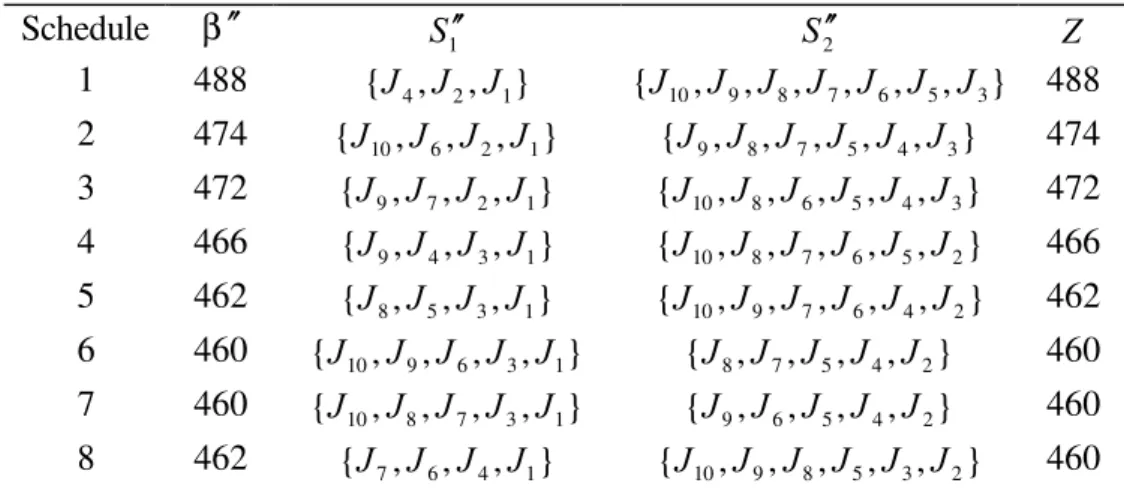
, and terminate the search as optimal solution has been found. The proposed algorithm returns a total flowtime of 575, which is 6.26% lower than that of the TMO algorithm.

Table 1. Example 2: Schedules where

α

*

=

105 Schedule

β ′′

S

₁

′′

S

₂

′′

Z

1

488 {

J

₄

,

J

₂

,

J

₁

}

{

J

₁₀

,

J

₉

,

J

₈

,

J

₇

,

J

₆

,

J

₅

,

J

₃

}

488

2

474 {

J

₁₀

,

J

₆

,

J

₂

,

J

₁

}

{

J

₉

,

J

₈

,

J

₇

,

J

₅

,

J

₄

,

J

₃

}

474

3

472 {

J

₉

,

J

₇

,

J

₂

,

J

₁

}

{

J

₁₀

,

J

₈

,

J

₆

,

J

₅

,

J

₄

,

J

₃

}

472

4

466 {

J

₉

,

J

₄

,

J

₃

,

J

₁

}

{

J

₁₀

,

J

₈

,

J

₇

,

J

₆

,

J

₅

,

J

₂

}

466

5

462 {

J

₈

,

J

₅

,

J

₃

,

J

₁

}

{

J

₁₀

,

J

₉

,

J

₇

,

J

₆

,

J

₄

,

J

₂

}

462

6

460 {

J

₁₀

,

J

₉

,

J

₆

,

J

₃

,

J

₁

}

{

J

₈

,

J

₇

,

J

₅

,

J

₄

,

J

₂

}

460

7

460 {

J

₁₀

,

J

₈

,

J

₇

,

J

₃

,

J

₁

}

{

J

₉

,

J

₆

,

J

₅

,

J

₄

,

J

₂

}

460

8

462 {

J

₇

,

J

₆

,

J

₄

,

J

₁

}

{

J

₁₀

,

J

₉

,

J

₈

,

J

₅

,

J

₃

,

J

₂

}

460

Example 2 consists of ten jobs and their processing times are: 8, 46, 30, 19, 4, 36, 21, 23, 6, and 17. We arrange the jobs in LPT order to

p

₁ = 46,

p

₂= 36,

p

3 = 30,

p

4 = 23,

p

5 = 21,

p

6 =

19,

p

7 = 17,

p

8 = 8,

p

9 = 6, and

p

10 = 4. Solving the problem using TMO gives

)

,

(

₄ ₂ ₁

1

J

S

=

,

S

₂=

(

J

₁₀

,

J

₉

,

J

₈

,

J

₇

,

J

₆

,

J

₅

,

J

₃

)

,

α

* = 105, and

β

= 488. We formulate the alternative problem with

d

_i = {10, 7, 2, 9, 2} and using the procedure in Section 3.2, we solve the

P

2 ||

F

_h

(

C

_max

∑

C

_i

)

problem to get its optimal solution as

)

,

(

9 8 5 4 1

1

J

S

′

=

,

S

2

′

=

(

J

10

,

J

7

,

J

6

,

J

3

,

J

2

)

,

α

=106, and

(9)

Since

α ≠

α

*, we use algorithm M to find an optimal solution. The schedules generated by the application of algorithm M are shown in Table 1 and result in an optimal schedule with

β

* = 460 when makespan

α

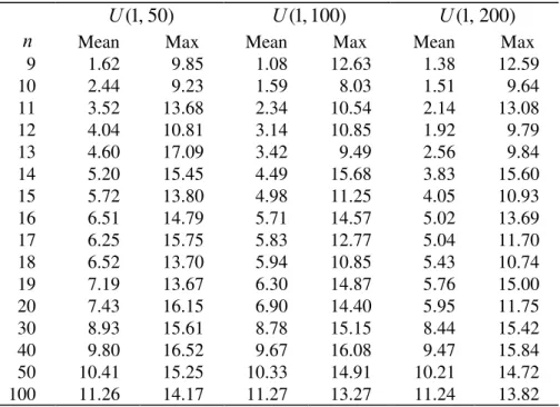
* = 105.

Table 2. Mean and maximum percent deviations using the TMO algorithm

)

50 ,

1 (

U

(

1 ,

100 )

U

(

1 ,

200 )

n

Mean Max Mean Max Mean Max

9 1.62 9.85 1.08 12.63 1.38 12.59

10 2.44 9.23 1.59 8.03 1.51 9.64

11 3.52 13.68 2.34 10.54 2.14 13.08

12 4.04 10.81 3.14 10.85 1.92 9.79

13 4.60 17.09 3.42 9.49 2.56 9.84

14 5.20 15.45 4.49 15.68 3.83 15.60

15 5.72 13.80 4.98 11.25 4.05 10.93

16 6.51 14.79 5.71 14.57 5.02 13.69

17 6.25 15.75 5.83 12.77 5.04 11.70

18 6.52 13.70 5.94 10.85 5.43 10.74

19 7.19 13.67 6.30 14.87 5.76 15.00

20 7.43 16.15 6.90 14.40 5.95 11.75

30 8.93 15.61 8.78 15.15 8.44 15.42

40 9.80 16.52 9.67 16.08 9.47 15.84

50 10.41 15.25 10.33 14.91 10.21 14.72

100 11.26 14.17 11.27 13.27 11.24 13.82

4. Computational Results

A simulation experiment was performed to evaluate the effectiveness of the proposed algorithm by comparing the value of its total flowtime to that found by using the TMO algorithm. The TMO algorithm was selected since it guarantees the optimal makespan, which is a requirement of the problem considered in this paper. In addition, we also compared the optimal values of the total flowtime for the

P

2 ||

F

h

(

∑

C

i

C

max

)

and

P

2 ||

∑

C

i problems.

We considered two factors in the simulation study: the number of jobs and the variability of processing times. The number of jobs was set in 16 levels: 9, 10, 11, 12, 13, 14, 15, 16, 17, 18, 19, 20, 30, 40, 50, and 100. The processing times were generated from a uniform distribution,

)

,

(

a

b

U

, and set at three levels:

U

(

1 ,

50 ),

U

(

1 ,

100 ),

and

U

(

1 ,

200 ).

The uniform distribution was chosen because it is commonly used in the literature. These two factors give a total of 48 sets of problems. For each set of problems, 100 replications are made. Hence, a total of 4,800 problems are solved. All algorithms were programmed in Microsoft FORTRAN running on an Intel Pentium-based microcomputer.

(10)

For each problem, we computed the percentage deviation of the total flowtime obtained using the TMO algorithm from the optimum total flowtime value found by algorithm E. For each set of problems, we report the mean and maximum percent deviations for TMO. Moreover, we tabulate the percentage of the time that the proposed algorithm E outperforms TMO for each set of problems.

Table 2 gives the mean and maximum percent deviations of the total flowtime using the TMO algorithm from the optimal total flowtime. From Table 2, it is clear that as the number of jobs increases, both mean and maximum percent deviations tend to increase. The three largest mean percent deviations occur when

n

= 100. Moreover, results in Table 2 show that as the variability of processing times decreases, the mean percent deviation figures increase in every case except the following two cases: when

n

= 9 and from

U

(

1 ,

200 )

to

U

(

1 ,

100 ),

and

n

= 100 and from

U

(

1 ,

100 )

to

U

(

1 ,

50 ).

The averages of the mean percent deviation figures for

),

50 ,

1 (

U

(

1 ,

100 ),

and

U

(

1 ,

200 )

are 6.34%, 5.74%, 5.25%, respectively. The maximum percent deviation figures also tend to increase as variability of processing times decreases, though not as pronounced as the mean percent deviation. In summary, results in Table 2 show that the use of proposed algorithm E significantly improves the total flowtime of the minimum makespan schedule obtained by the TMO algorithm.

Table 3 reports the percentage of problems that the proposed algorithm outperforms the TMO. Similar to the conclusions obtained from Table 2, Table 3 shows that as the number of jobs increases or/and variability of processing times decreases, the proposed algorithm E becomes more effective since the percent of problems for which TMO fails to find optimal total flowtime schedules increases. The proposed algorithm E always returns a smaller total flowtime than the TMO when

n

= 14. On average, the proposed algorithm outperforms the TMO algorithm for

),

50 ,

1 (

U

(

1 ,

100 ),

and

U

(

1 ,

200 )

in 96.1%, 93.6%, and 91.3% of the problems, respectively.

Table 3. Percentage of problems the TMO algorithm yields a larger total flowtime

n

U

(

1 ,

50 )

U

(

1 ,

100 )

U

(

1 ,

200 )

9 62 47 48

10 83 64 57

11 92 87 75

12 100 100 86

13 100 99 95

14 100 100 100

15 100 100 100

16 100 100 100

17 100 100 100

18 100 100 100

19 100 100 100

20 100 100 100

30 100 100 100

40 100 100 100

50 100 100 100

100 100 100 100

(11)

4.2. Optimal Flowtimes for the

P

2 ||

F

_h

(

∑

C

_i

C

_max

)

and

P

2 ||

∑

C

_i Problems

For each problem size and dataset, the mean and maximum percentage deviations of the optimal flowtime value for the

P

2 ||

F

h

(

∑

C

i

C

max

)

problem from that for the

P

2 ||

∑

C

i problem are shown in Table 4

Table 4. Mean and maximum percent deviations of the optimal flowtime value for the

)

(

||

2 F

∑

C

_max

P

_h _i problem from that for the

P

2 ||

∑

C

_i problem

)

50 ,

1 (

U

(

1 ,

100 )

U

(

1 ,

200 )

n

Mean Max Mean Max Mean Max

9 0.287 3.044 0.677 7.730 0.882 7.726

10 0.367 5.791 0.622 5.882 0.936 6.500

11 0.089 1.206 0.156 1.613 0.248 1.690

12 0.049 0.708 0.107 1.407 0.267 2.281

13 0.038 0.620 0.049 0.656 0.105 1.680

14 0.026 0.593 0.052 0.861 0.088 0.760

15 0.002 0.207 0.006 0.159 0.016 0.417

16 0.000 0.000 0.003 0.110 0.005 0.137

17 0.002 0.147 0.004 0.214 0.005 0.199

18 0.002 0.080 0.002 0.159 0.002 0.046

19 0.001 0.084 0.001 0.086 0.001 0.065

20 0.001 0.067 0.001 0.049 0.001 0.051

30 0.000 0.000 0.000 0.000 0.000 0.000

40 0.000 0.000 0.000 0.000 0.000 0.000

50 0.000 0.000 0.000 0.000 0.000 0.000

100 0.000 0.000 0.000 0.000 0.000 0.000

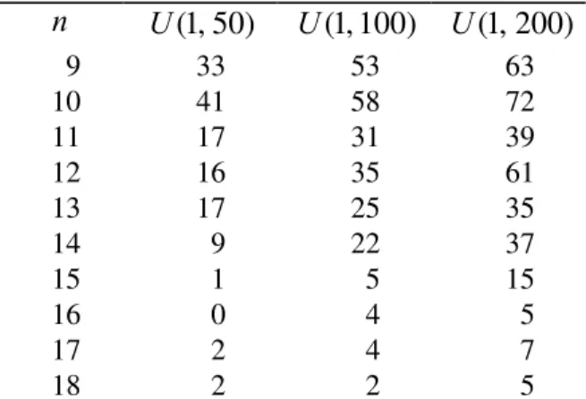
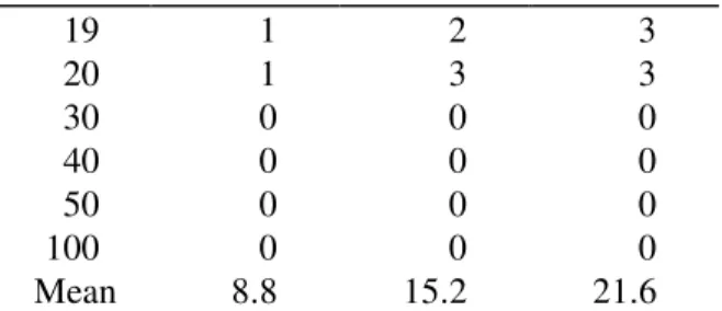
Table 5. Percentage of problems the proposed algorithm is sub-optimal for the

P

2 ||

∑

C

_i problem

n

U

(

1 ,

50 )

U

(

1 ,

100 )

U

(

1 ,

200 )

9 33 53 63

10 41 58 72

11 17 31 39

12 16 35 61

13 17 25 35

14 9 22 37

15 1 5 15

16 0 4 5

17 2 4 7

(12)

19 1 2 3

20 1 3 3

30 0 0 0

40 0 0 0

50 0 0 0

100 0 0 0

Mean 8.8 15.2 21.6

In addition, Table 5 shows the percentage of the problems for which this percentage deviation was greater than zero. From these results, it is clear that the total flowtime for the two problems can be quite different. Hence, use of the proposed algorithm E is useful.

Table 6 Set CPU time (in seconds)

)

50 ,

1 (

U

(

1 ,

100 )

U

(

1 ,

200 )

n

TMO Proposed TMO Proposed TMO Proposed

9 0.10 0.15 0.00 0.10 0.10 0.10

10 0.10 0.15 0.05 0.10 0.05 0.20

11 0.05 0.10 0.05 0.20 0.10 0.25

12 0.05 0.15 0.00 0.20 0.00 0.40

13 0.05 0.20 0.15 0.35 0.10 0.30

14 0.05 0.25 0.00 0.35 0.10 0.55

15 0.10 0.20 0.00 0.20 0.05 0.55

16 0.10 0.15 0.05 0.25 0.15 0.35

17 0.10 0.30 0.25 0.50 0.25 0.76

18 0.05 0.47 0.20 0.57 0.05 1.05

19 0.05 0.47 0.10 0.69 0.10 1.28

20 0.05 1.07 0.05 1.88 0.20 1.83

30 0.15 0.20 0.10 0.20 0.15 0.20

40 0.15 0.25 0.25 0.35 0.25 0.40

50 0.10 0.40 0.20 0.45 0.25 0.40

100 0.65 1.25 0.60 1.25 0.65 1.30

(13)

4.3 Efficiency of the Proposed Algorithm

For each problem set, Table 6 gives CPU time for the TMO and the proposed algorithms. It shows that the solution of 100 problems in each set, the TMO and proposed algorithms on average require 0.135 and 0.486 seconds, respectively. Nonetheless, the proposed algorithm is very fast and can be used to solve both large and small size problems. For example, the largest set CPU time of the proposed algorithm is just 1.88 seconds when

n

= 20. One very interesting observation concerning the number of jobs factor is the fact that the CPU time of the proposed algorithm increases as

n

increases from 9 to 20, then it decreases when

n

increases from 20 to 30 and increases again when

n

increases from 30 to 100. This is because when 20 <

n

< 30, the probability that the proposed algorithm terminates in Step 2, due to the condition that

*

α

α =

, becomes very high (almost 100%) and remains stable. Thus, the CPU time therefore goes down. When

n

> 30, the increase in CPU time is purely due to the increase in the number of jobs. Furthermore, results in Table 6 show a positive correlation between processing time variability and CPU time.

5. Conclusions

This paper considered the two-identical-parallel-machine problem to minimize total flowtime subject to minimum makespan and proposed an optimization algorithm for its solution. Computational results of a simulation study with randomly generated problems show that the proposed optimization algorithm E is quite efficient in optimizing large-sized problems. On the average, for the three cases of processing times variability

U

(

1 ,

50 ),

U

(

1 ,

100 ),

and

),

200 ,

1 (

U

the total flowtime value obtained by proposed algorithm E are 6.34%, 5.74%, 5.25% less than those found using the TMO algorithm, respectively. The computational results also indicate that the proposed algorithm, which finds optimal total flowtime, outperforms the TMO in all 48 sets of problems. Furthermore, the proposed algorithm returns a smaller total flowtime than that of TMO in 93.65% of the 4,800 test problems. In terms of CPU time, both algorithms are very efficient, the mean CPU time per set of 100 problems for the proposed and TMO algorithms are 0.486 and 0.135 second, respectively.

Several issues are worthy of future investigations. First, extension of results to the m -identical-parallel-machine case (

m

> 2) will be worthwhile. Second, the solution of the problem with the reverse hierarchical optimality criteria, namely, the identical-parallel-machine scheduling problem where the primary criterion is the minimization of the total flow-time and the secondary criterion is the minimization of the maximum completion time (makespan) is both interesting and useful. Third, the development of algorithms for other secondary criteria such as the total tardiness subject to the minimum makespan is a fruitful area of research. Finally, extension of our results to more complex machine environments, such as multi-stage flowshop and job-shop problems, is important for application in industry.

References

(1) Bruno, J., Coffman, E.G., & Sethi, R. (1974). Scheduling independent tasks to reduce mean finishing time. Communications of the ACM, 17, 382-387.

(14)

(3) Conway, R.W., Maxwell, W.L., & Miller, L.W. (1967). Theory of Scheduling. Addison Wesley, Reading, MA.

(4) Eck, B.T., & Pinedo, M. (1993). On the minimization of the makespan subject to flowtime optimality. Operations Research, 41, 797-800.

(5) Garey, M.R. & Johnson, D.S. (1979). Computers and Intractability: A Guide to the Theory of NP-Completeness. Freeman, San Francisco, CA.

(6) Ho, J.C., & Wong, J.S. (1995). Makespan minimization for parallel identical processors. Naval Research Logistics, 42, 935-948.

(7) Lee, C.-Y. & Vairaktarakis, G.L. (1993). Complexity of single machine hierarchical scheduling: a survey. In:Complexity in Numerical Optimization [edited by P.M. Pardalos], World Scientific Publishing Company, 269-298.

(8) McNaughton, R. (1959). Scheduling with deadlines and loss functions, Management Science, 6, 1-12.